A Novel Generalized Ridge Regression Method
for Quantitative Genetics
Xia Shen,*,†,1Moudud Alam,†Freddy Fikse,‡and Lars Rönnegård†,‡ *Division of Computational Genetics, Department of Clinical Sciences and‡Department of Animal Breeding & Genetics, Swedish University of Agricultural Sciences, 75007 Uppsala, Sweden, and†Statistics, School of Technology and Business Studies, Dalarna University, 78170 Borlänge, Sweden
ABSTRACTAs the molecular marker density grows, there is a strong need in both genome-wide association studies and genomic selection tofit models with a large number of parameters. Here we present a computationally efficient generalized ridge regression (RR) algorithm for situations in which the number of parameters largely exceeds the number of observations. The computationally demanding parts of the method depend mainly on the number of observations and not the number of parameters. The algorithm was implemented in the R packagebigRRbased on the previously developed packagehglm. Using such an approach, aheteroscedastic
effects model(HEM) was also developed, implemented, and tested. The efficiency for different data sizes were evaluated via
simu-lation. The method was tested for a bacteria-hypersensitive trait in a publicly availableArabidopsisdata set including 84 inbred lines and 216,130 SNPs. The computation of all the SNP effects required,10 sec using a single 2.7-GHz core. The advantage in run time makes permutation test feasible for such a whole-genome model, so that a genome-wide significance threshold can be obtained. HEM was found to be more robust than ordinary RR (a.k.a. best linear unbiased prediction) in terms of QTL mapping, because SNP-specific shrinkage was applied instead of a common shrinkage. The proposed algorithm was also assessed for genomic evaluation and was shown to give better predictions than ordinary RR.
H
IGH-dimensional problems are increasing in importance in genetics, computational biology, and other fields of research where technological developments have greatly facilitated the collection of data (Hastie et al. 2009). In genome-wide association studies (GWAS) and genomic selection (GS), the number of observationsnis generally in the order of hundreds/thousands whereas the number of marker effects to befittedpis in the order of hundreds of thousands. This is a rather extreme p n problem, and the methods developed for analyses of the data need to be computationally feasible. At the same time the mod-elsfitted should beflexible enough to capture the impor-tant genetic effects that are often quite small (Hayes and Goddard 2001).Methodologies regarding high-dimensional genomic data focus on bothdetectionandpredictionpurposes. There is currently a trend that GWAS and GS could potentially apply the same framework of models. Such models fit the whole
genome based on penalized likelihood or Bayesian shrinkage estimation (see the review by de los Camposet al.2013). Or-dinary GWAS usually avoids high-dimensional models and turns the problem into multiple testing instead (e.g., the review by Kingsmoreet al.2008). The tests of all the SNPs (single nucle-otide polymorphisms) are dismembered. Such routine sacrifices both detective and predictive power. Using detected QTL (quan-titative trait loci that are genome-wide significant), the predic-tion can be rather poor, which led to the insignificant application of marker-assisted selection (MAS) (Dekkers 2004). GS, how-ever, has been practically useful by incorporating a large amount of small genetic effects unmappable from GWAS or QTL analy-sis. There are a number of whole-genome models where not only the individual predictors (breeding values) but also the SNP effects can be estimated,e.g., SNP–best linear unbiased prediction (BLUP) and different kinds of Bayesian models (e.g., Meuwissen et al. 2001; Xu 2003; Yi and Xu 2008; Gianolaet al.2009; Habieret al.2011). The whole genome models are powerful; nevertheless, there are problems that limit its wide usage: (1) computation for these models in-cluding all the SNPs can be intensive, whereas efficiency is required in practice so that prediction can be obtained in early life of the individuals (de los Campos et al. 2013); Copyright © 2013 by the Genetics Society of America
doi: 10.1534/genetics.112.146720
Manuscript received October 11, 2012; accepted for publication January 9, 2013
1Corresponding author: Swedish University of Agricultural Sciences, Box 7078, 75007
Uppsala, Sweden. E-mail: [email protected]
(2)fittinglarge-p small-nmodels requires variable selection or shrinkage estimation, and the significant threshold for the shrinkage estimates of SNP effects is difficult to specify, which is an issue that limits the usage of such models in gene mapping; and (3) thefitting of Bayesian models is performed using randomization/simulations, where in application, mix-ing of the Markov chain Monte Carlo (MCMC) algorithm can become poor in case of high-dimensional models.
Linear mixed models (LMM) have been proposed for GS (SNP-BLUP; Meuwissen et al. 2001) and ridge regression (RR) for GWAS (Maloet al.2008). LMMs and RR are fun-damentally the same since they fit a penalized likelihood using a quadratic penalty function (see the Appendix for more details). It is well established (Hastieet al.2009) that RR can befitted forpnin a computationally efficient way using singular-value decomposition (SVD) of the design ma-trix, which, for instance, has been applied to expression arrays in genetics (Hastie and Tibshirani 2004). However, this approach assumes that the RR shrinkage parameter is constant for all p fitted parameters. In generalized RR the shrinkage parameter may vary between the parameters (Hoerl and Kennard 1970a,b). In both multilocus GWAS and GS, it is not reasonable to assume that shrinkage should be constant for allfitted SNP effects over the entire genome. This is be-cause neither the gene effects are normally distributed nor are most markers linked to any functional gene (Meuwissenet al. 2001). To allow SNP-specific shrinkage, the previously men-tioned Bayesian methods were developed.
There is a need for a method that isfast(efficient to per-form),testable(can produce a genome-wide significance thresh-old for association study),deterministic(the same estimates are easy to replicate), and flexible(SNP-specific shrinkage can be easily applied). The aim of this article is to develop such a gen-eralized RR method, which will be referred to as the
heterosce-dastic effects model (HEM), for p n high-dimensional
problems, based on LMM theory. HEM approximates a previ-ously proposed method (Rönnegård and Lee 2010; Shenet al. 2011) that was based on double hierarchical generalized linear models (DHGLM; Lee and Nelder 2006), but with a tremendous increase in computational speed for p n problems. An important contribution of the theory presented is a fast transformation of hat values (leverages) and prediction er-ror variances of the random effects. The method has been implemented in the R (R Development Core Team 2010) package bigRR (available at https://r-forge.r-project.org/ R/?group_id=1301).
Methods and Materials
Statistical models
Using Henderson’s mixed model equation:We start by introducing the normal RR as a LMM. The theoretical basis of the connection between RR and LMM is given in theAppendix. The SNP effects are estimated as random effects,i.e., so-called SNP–BLUP. We use the terms RR and SNP–BLUP interchange-ably in this article. Given a phenotype vectoryforn
individ-uals,fixed effects dataX,and the data forpSNPs along the genomeZ, the normal LMM for SNP–BLUP can be written as
y¼XbþZbþe; (1)
wherebNð0;s2
bIpÞ,eNð0;s2eInÞ,bis the vector offixed effects, andbis the vector of random SNP effects. The matrix
Z haspcolumns for the SNPs where each column is usually coded as 0, 1, and 2, for the homozygoteaa, the heterozygote Aa, and the other homozygote AA, respectively. However, here, we standardize the coding for Z based on VanRaden (2008) using the allele frequencies. This is essential in RR problems since the sizes of the estimated effects need to be comparable. Although the models are introduced in the simple normal LMM notation, the method is developed for general-ized distributions of phenotypes (see also Fitting algorithm and theAppendix).
It is well known that the fixed effects b and random effects b can be estimated jointly via Henderson’s mixed model equation (MME; Henderson 1953)
X9X X9Z Z9X Z9ZþlI
b b
¼
X9y Z9y
; (2)
where l¼s^2
e=^s2b, determined by the variance component estimators, is the shrinkage parameter for the random SNP effects.lis analogous to the one in the penalized likelihood for RR. In terms of estimating SNP effects for QTL mapping, such an MME for RR is not appropriate because the same magnitude of shrinkage is applied to all the SNPs (Xu 2003). Hence, the markers are regardeda prioriwith no difference. Since most of the loci in the genome are supposed to con-tribute little to the observed phenotype, those SNPs should be penalized more in the analysis. This is one of the funda-mental ideas from which the current Bayesian methods are developed (e.g., Meuwissenet al.2001; Xu 2003).
From (2), it is clear that to obtain different shrinkage for different SNPs, the lIpart should be replaced so that thep numbers on the diagonal are not identical. An essential ques-tion here is how much shrinkage should be given to each SNP. We propose a generalized RR solution to this problem, which is presented as the following HEM. We use the MME andfit a generalized RR after the ordinary RR in (2).
X9X X9Z
Z9X Z9ZþdiagðlÞ
b b
¼
X9y Z9y
; (3)
where lis a vector of p shrinkage parameters with its jth element lj¼s^2e=^s
2
bj. The SNP-specific variance component ^
s2
bj is calculated as
^ s2
bj¼
^
b2j
12hjj;
(4)
T¼
X Z
0 diagðlÞ
: (5)
Such a quantity (4) is useful because it (1) directly tells how much shrinkage should be given to each SNP and (2) makes the entire procedure deterministic and repeatable. This simple way of setting the shrinkage parameters is an approximation of previously established theory for double hierarchical general-ized linear models (Lee and Nelder 2006) applied in Rönnegård and Lee (2010) and Shenet al.(2011), wherebjdepended on a second-layer model including random effects and was esti-mated iteratively until convergence. Using (4) the shrinkage for each SNP in HEM is computed directly without iteration.
Transformation via the animal model: Stranden and Garrick (2009) showed that the computations for an animal
modelincluding a genomic relationship matrix is equivalent to
fitting an LMM including random SNP effects. Below we ex-ploit this fact to derive the algorithm for HEM. A major con-tribution of the theory below is the derivation of a simple equation to compute the hat values for the SNP effects from the hat values for the animal effects (in step 5 ofFitting
algo-rithmbelow). It should also be noted that the generalized RR
part of the HEM algorithm does not use singular-value decom-position as proposed by Hastie and Tibshirani (2004) and
Has-tieet al.(2009) and described in theAppendix, but rather uses
transformation between equivalent models as described below. From (3) and (4), the generalized RR method, HEM, is quite easy to describemathematically. However, to obtain esti-mated effects for all the SNPs, the matrixZ9Z+ diag(l) (size p·p) is too large to invert. So we need to make the equations
computationallysimple. This can be done by connecting (3) to
an animal model. Let us defineG =ZZ9, which is a matrix representing genomic kinship that indicates the relatedness between individuals. The animal model
y¼Xbþaþe (6)
containsaNð0;Gs2
aÞas random effects fornindividuals. The size of the MME for such an animal model is much smaller than (2), i.e.,
X9X X9
X IþlG21
b a
¼
X9y
y
: (7)
Because of the mathematical equivalence, thelin (7) is iden-tical to that in (2). In fact, there is no need to directlyfit the MME (2) or (3) because all the information that links the estimated individual effects ^ato the SNP effects ^b are con-tained in the single genotype matrixZ. Afterfitting the animal model via (7), one can show that the following transformation holds (e.g., Pawitan 2001, p. 446),
^
b¼Z9G21a^; (8)
where only the matricesZ9(sizep·n) andG21(sizen·n) are required, given that Gis full ranked. Sincen p, the
MME (2) and HEM (3) can be solved a lot faster by the “animal model (7) + transformation (8)”procedure. For HEM, the hat value for each SNP is required in the MME (3), and we show that fortunately, a similar transforma-tion can be applied for transforming the hat values of the animal effects to the SNP effects as well (see Fitting
al-gorithm and the Appendix). Besides the efficiency, by
avoiding huge matrices, a significant amount of memory can be saved so that almost any large number of SNPs can be loaded simultaneously.
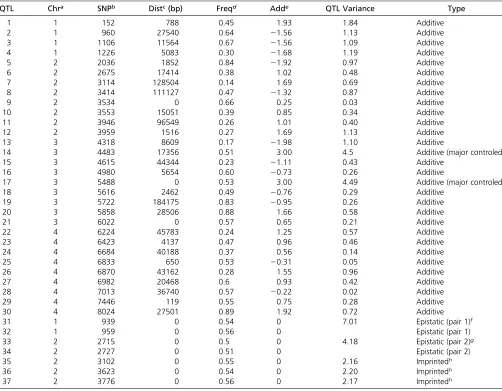
To evaluate the run time forfitting a linear mixed model or RR using our algorithm, we simulated a standard-normally distributed phenotype with sample sizes varied from 100 to 1000. Marker genotypes were also simulated and the number of markers varied from 10K to 1M.
Fitting algorithm
Below we present thefitting algorithm for HEM. Steps 1–4 fit SNP–BLUP and steps 5–8fit a generalized RR. The algo-rithm also includes a Cholesky decomposition of the geno-mic relationship matrixGto simplify the computations and the transformation of hat values (in step 5).
Given a phenotype vectory(sizen·1) that belongs to any GLM (generalized linear model) family, e.g., binary, poisson, gamma, etc., fixed effects design matrixX (size n·k), the SNP genotype matrixZ(sizen·p), the SNP– BLUP (RR), and HEM (generalized RR) can be computed as follows:
1. Calculate G = ZZ9, its Cholesky decomposition L s.t.
LL9=G, and its inverseG21.
2. Fit a GLMM with responsey,fixed effectsXand random effects design matrix L. Because of mathematical equiv-alence, this fits the animal model (6) as a GLMM with correlated random effects.
3. From step 2, store the estimated variance componentss^2b, ^
s2
e, and the animal effectsa^. Calculatel¼s^ 2 e=^s
2 b. 4. Transform^aback to the SNP effects^b¼Z0G21^a. 5. Define
Cv¼
1 ^ s2
e
X9X X9L L9X L9LþlIn
(9)
and divide the inverse ofCvinto blocks
C1
v ¼
C11
v C12v
C21
v C22v
!
: (10)
Define a transformation matrixM =Z9G21L. Calculate the hat value for each random SNP effect as
hjj¼12Mj
In2C22v =^s2b
M9j; (11)
whereMjis thejth row of the transformation matrix M.
wjj¼
^
b2j
12hjj
(12)
and updateGto beG* =ZWZ9. CalculateG*21, andL*s.t.
L*L*9¼G*.
7. Fit a GLMM with responsey,fixed effectsX,and random effects design matrixL*.
8. From step 7, transform the updated individual effectsa^ back to the SNP effectsb^¼Z9G*21^a.
In this algorithm, GLMMs are estimated based on penalized quasi-likelihood (PQL) for MME (see R package hglmand its algorithm in Rönnegårdet al.2010). To be comparative to MME for normal LMM, the notation s2
e is used in the algorithm even for GLMM to denote the residual dispersion parameter. Theoretical details about the transformations are given in theAppendix.
Randomization test
Specifying a significance threshold for any whole genome model has been a challenging problem. The predictors in LMM or GLMM for the random effects (i.e., BLUP) have“prediction errors”(e.g., Pawitan 2001), which could be used to construct “t-like”statistics. But this is properly applicable only when the number of random effects predictors is small, namely, when shrinkage does not affect much of the test statistic distribution since the random effects estimates are not so different from those if all the effects are estimated as fixed. But this is not proper anymore when the number of explanatory variables or genetic markers is much more than the number of individuals, because the estimated effects are too much biased from their real genetic effects (Zeng 1993; Rodolphe and Lefort 1993). So when a whole genome of markers is fitted together, the model ends up with too much shrinkage to make thet -distri-bution hold. Hence, current Bayesian methods (e.g., Xu 2003) just set up an empirical LOD score threshold (e.g., Che and Xu 2012) using the suggestions by Kidd and Ott (1984) and Risch (1991). Nevertheless, the genome-wide significance test can actually be practically important. Here, randomization/per-mutation is a solution if the computation is not too intensive forfitting all the markers. Since the HEM algorithm proposed in this article is computationally efficient, a genome-wide sig-nificance threshold can be determined by randomization test. In the analysis of theArabidopsis thalianaGWAS data using HEM, the permutation test was performed to determine a 5% genome-wide significance threshold for QTL detection, where the phenotype was permuted 1000 times, and the 95% quan-tile of the maximum effects was calculated as the threshold.
Data
We applied HEM on three data sets. Using HEM, we searched for significant SNPs in a publicly availableA. thali-anaGWAS data set. In the other two data sets the predictive power of HEM in GS was assessed.
A. thaliana GWAS data: Atwell et al. (2010) performed GWA studies for 107 phenotypes of A. thaliana and success-fully detected a set of candidate genes. Using the heterosce-dastic effects model, we analyzed one defense-related binary trait out of their 107 published phenotypes: hypersensitive re-sponse to the bacterial elicitor AvrRpm1. The reason for choos-ing this trait is because it is under regulation of a known candidate geneRPM1and so we can validate our HEM method in terms of QTL detection. A total of 84 ecotypes were pheno-typed (28 controls and 56 cases). The genotype data are from a 250K SNP chip including 216 130 available SNPs (http:// arabidopsis.usc.edu).
GSA common simulated data:To compare different newly developed genomic evaluation methods, the Genetics Soci-ety of America (GSA) provides several common data sets for authors to analyze and report their results (Hickey and Gorjanc 2012). We chose the simulated livestock data struc-ture to assess our method.
The total number of segregating sites across the genome was approximately 1.67 million. A random sample of 60,000 segregating sites was selected from the sequence to be used as SNPs on a 60K SNP array. In addition, a set of 9000 segregating sites were randomly selected from the sequence to be used as candidate QTL in two different ways: (1) a randomly sampled set, and (2) a randomly sampled set with the restriction that their minor allele frequencies (MAFs) should not exceed 0.30. Four different traits were simulated, assuming an additive genetic model. The first pair of traits was generated using the 9000 unrestricted QTL. For thefirst trait (PolyUnres), the allele substitution effect at each QTL was sampled from a standard normal distribution. For the second trait (GammaUnres) a ran-dom subset of 900 of the candidate QTL was selected with allele substitution effects sampled from a gamma distribution with a shape parameter of 0.4, scale parameter of 1.66 (Meuwissen
et al.2001), and a 50% chance of being positive or negative. The
second pair of traits (PolyRes and GammaRes) was generated in the same way as the first pair except that the candidate QTL have the restriction that their MAF not be .0.30. Phenotypes with a heritability of 0.25 were generated for each trait.
Training and validation subsets of the data were extracted for training and validation. The training set comprised the 2000 individuals in generations 4 and 5. The validation set comprised 1500 individuals sampled at random from generation 6, 8, and 10 (500 individuals from each generation). Wefit a whole-genome model using HEM and compare the prediction performance in the validation data set.
(F4 generation, individuals 2327–3226) had no phenotypic records. The genome was about 500-Mb long, consisting of five chromosomes, each of which contained about 100 Mb. Each individual was genotyped for 10,031 biallelic SNPs that densely distributed along the genome. Regarding recombina-tion rate, 1 cM was assumed to be 1 Mb; therefore, the size of the genome is about 500 cM.
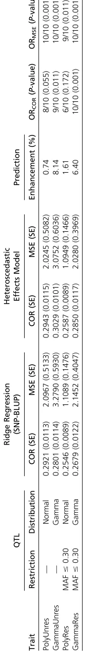
Thirty-seven QTL were simulated along the genome, and no QTL existed on chromosome 5 (Table 1). All the QTL con-trolled QT, including 30 additive loci, 2 epistatic pairs, and 3 imprinted loci. Of the 30 additive QTL, 22 also controlled BT, namely that pleiotropic effects existed for the two traits. QT was mainly controlled by additive QTL 14 and 17, as well as the two epistatic pairs. BT was mainly controlled by additive QTL 14. Due to epistasis and imprinting, QT had a more complicated
genetic architecture than BT. We have published (Shenet al. 2011) our previous analysis of this data set using a DHGLM (Lee and Nelder 2006). Considering HEM as a simple and efficient substitution of DHGLM, we reanalyzed the data byfitting all the markers and compared the results with the previous results.
Results
Computational efficiency
On a single Intel Xeon E5520 2.27-GHz CPU, the computation was fast, especially when the number of individuals was small (Figure 1), since the computation-demanding parts in the algorithm depend mainly on the sample size. For a population with 100 individuals, even when there are 1 million markers, estimation of all the effects along the genome takes,2 min. Table 1 Genetic models of simulated quantitative trait for the QTLMAS 2010 data (Szydlowski and Paczy ´nska 2011)
QTL Chra SNPb Distc(bp) Freqd Adde QTL Variance Type
1 1 152 788 0.45 1.93 1.84 Additive
2 1 960 27540 0.64 21.56 1.13 Additive
3 1 1106 11564 0.67 21.56 1.09 Additive
4 1 1226 5083 0.30 21.68 1.19 Additive
5 2 2036 1852 0.84 21.92 0.97 Additive
6 2 2675 17414 0.38 1.02 0.48 Additive
7 2 3114 128504 0.14 1.69 0.69 Additive
8 2 3414 111127 0.47 21.32 0.87 Additive
9 2 3534 0 0.66 0.25 0.03 Additive
10 2 3553 15051 0.39 0.85 0.34 Additive
11 2 3946 96549 0.26 1.01 0.40 Additive
12 2 3959 1516 0.27 1.69 1.13 Additive
13 3 4318 8609 0.17 21.98 1.10 Additive
14 3 4483 17356 0.51 3.00 4.5 Additive (major controled)
15 3 4615 44344 0.23 21.11 0.43 Additive
16 3 4980 5654 0.60 20.73 0.26 Additive
17 3 5488 0 0.53 3.00 4.49 Additive (major controled)
18 3 5616 2462 0.49 20.76 0.29 Additive
19 3 5722 184175 0.83 20.95 0.26 Additive
20 3 5858 28506 0.88 1.66 0.58 Additive
21 3 6022 0 0.57 0.65 0.21 Additive
22 4 6224 45783 0.24 1.25 0.57 Additive
23 4 6423 4137 0.47 0.96 0.46 Additive
24 4 6684 40188 0.37 0.56 0.14 Additive
25 4 6833 650 0.53 20.31 0.05 Additive
26 4 6870 43162 0.28 1.55 0.96 Additive
27 4 6982 20468 0.6 0.93 0.42 Additive
28 4 7013 36740 0.57 20.22 0.02 Additive
29 4 7446 119 0.55 0.75 0.28 Additive
30 4 8024 27501 0.89 1.92 0.72 Additive
31 1 939 0 0.54 0 7.01 Epistatic (pair 1)f
32 1 959 0 0.56 0 Epistatic (pair 1)
33 2 2715 0 0.5 0 4.18 Epistatic (pair 2)g
34 2 2727 0 0.51 0 Epistatic (pair 2)
35 2 3102 0 0.55 0 2.16 Imprintedh
36 2 3623 0 0.54 0 2.20 Imprintedh
37 2 3776 0 0.56 0 2.17 Imprintedh
aChromosome number. No QTL on chromosome 5. bThe closest SNP marker index.
cDistance from the QTL to the closest SNP marker. dFrequency of allele 1.
eAdditive effect: half the difference between homozygote means.
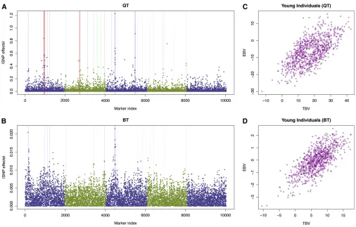
Analysis of the Arabidopsis data
For the 84 individuals and 216,130 informative markers on the
Arabidopsistrait AvrRpm1, the shrinkage effect was much
stron-ger for HEM than SNP–BLUP (Figure 2). According to Atwell
et al.(2010), this defense-related trait is essentially
monogeni-cally controlled by the gene RPM1. The analysis via a whole-genome model should validate such a strong monogenic effect in terms of QTL detection. In Figure 2, 5% genome-wide signif-icance thresholds via permutation tests are provided for both SNP–BLUP and HEM. Here, SNP–BLUP is not appropriate for QTL mapping due to constant shrinkage along the genome (Xu 2003). By allowing different weights on different SNPs, HEM has the property that it shrinks the small effects down toward zero, highlights the QTL effects, and produces reasonable genome-wide significance threshold obtained by permutation testing.
HEM also produces better resolution in mapping the candidate gene. A close-up of the region surrounding the RPM1 gene on chromosome 3 shows that the SNP with the largest2log10P-value from the Wilcoxon GWAS (Atwell
et al.2010) also has the largest estimate from HEM, whereas
the second largest estimate is found 0.1 Mb away from
RPM1 (Figure 3). Hence, a ranking of the top estimates results in a similar ranking as for the2log10P-values from Atwellet al.’s GWAS, where HEM is better at separating the ranking of SNPs close to each other on the chromosome.
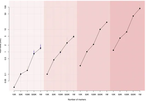
Analysis of the GSA simulated data
HEM is able tofit the entire 60K SNP chip on the GSA simulated data. We analyzed all the 10 replicates of the four simulated traits and performed the prediction using both SNP–BLUP and HEM (Table 2). It is not surprising that HEM is generally better in prediction than SNP–BLUP because of moreflexible shrink-age. It is noteworthy that such an advantage in prediction is clearer when the QTL effects are skewed (Gamma) than sym-metrically (Normal) distributed. This is because the SNPs that have major genetic effects are highlighted more by the HEM shrinkage compared to SNP–BLUP. This is a good property for HEM since most of the time, one would expect the genes to carry skewed genetic effects (Hayes and Goddard 2001).
Analysis of the QTLMAS data
Here we focus on breeding value estimation for the QTLMAS 2010 data set that was previously analyzed by Shen et al.
(2011). Due to the data size, the previous report could not fit all the markers into a DHGLM, but this is possible using HEM. Although HEM is theoretically an approximation of
DHGLM, it is not worse than our previous DHGLM method in terms of breeding value estimation where the strongest effects match the simulated true QTL very well (Figure 4). Figure 2 Estimated SNP effects for theArabidopsisbacteria-hypersensitive trait AvrRpm1 (Atwellet al.2010) using (A) ridge regression (SNP–BLUP) and (B) heteroscedastic effects model, which are plotted against each other in C. The horizontal dashed lines in A and B indicate the 5% genome-wide significance threshold from a randomization test using 1000 permutations.
Figure 3 The significant association peak for the
By taking into account all the markers in the genome, HEM was able to improve the prediction of the young individuals compared to DHGLM. It did as good as the previous DHGLM for the binary trait and gave a correlation between the true breeding values (TBV) and estimated breeding values (EBV) of 0.72, whereas for the quantitative trait, HEM successfully raised the correlation between TBV and EBV from 0.60 to 0.64 compared to our previous report (Shenet al. 2011).
Discussion
The presented generalized RR algorithm, HEM,fits models in which the number of parameterspis much greater than the number of observationsn. The focus of the article has been on applications in both GS and QTL detection, but the algorithm is expected to be of general use for applications of RR in other fields of research as well. The computational limitations of the
bigRRpackage come mainly from the number of observations, and not the number of parameters. In our implementation of the algorithm, we used thehglm package (Rönnegårdet al. 2010) in R for the variance component estimation, which is computationally feasible for data sets having up to 10,000 observations on a uni-core laptop computer. On any computer that has a CUDA-supported graphic card, an advanced version of the package can be required from the authors, which uti-lizes GPU for matrix calculation, accelerating the computation even more.
Compared to LMM and ordinary RR, the estimates from HEM are less sensitive to the assumption that the effects come from a common normal distribution and are therefore more robust. The method is computationally efficient due to its compression–decompression properties. In the Appendix, we show that theSNP-effects model(19) withpeffects to be esti-mated is compressed into an animal model (20) whose size depends on n. In the decompression part, the estimated SNP effects can quickly be estimated through a simple transforma-tion from individual effects to SNP effects. These estimates are used to update the matrix G, which is subsequently used in a compressed animal model. Thefinal estimates are then com-puted by decompressing the animal model once more.
RR is known to be able to address collinearity (Hoerl and Kennard 1970b). It avoids computational trouble for an ill-conditioned data matrix and also solves the problem due to ill-conditioned Fisher’s information matrix (e.g., in Poisson and binomial GLM) (Hastieet al.2009). In our analysis of
theArabidopsisdata, we found that HEM seems to have a good
performance in terms of correctlyfine-mapping functional loci. This suggests that when linkage disequilibrium (LD) exists around a QTL, a clearer signal could be identified, which is a good property of the method, although further investigations are required to verify this property of HEM. The improvement of a stronger feature selection method compared to RR depends on the underlying genetic architecture. For a trait with only a few QTL, an even stronger feature selection method, e.g., least absolute shrinkage and selection operator (LASSO) (Tibshirani 1996), may perform much better. However, many
complex traits, such as human height, have been shown to be very polygenic (e.g., Yanget al. 2011). At present, it is even more challenging in terms of both QTL mapping and genomic prediction when there are so many small and even undetect-able QTL.
The method combines two ideas from our earlier articles. First, in Rönnegård and Lee (2010) and Shenet al.(2011), a DHGLM (Lee and Nelder 2006) was proposed. This model fits SNP-specific variance components using a random effects model also for the second level in Equation 30 (see theAppendix). By introducing HEM as a simplification of the DHGLM, one achieves a dramatic gain in speed. Second, Christensen and Lund (2010) suggest in their dis-cussion that Gcould be weighted by a diagonal matrix D calculated from SNP effects and note, “However, incorpo-rating uncertainty on such estimated SNP effects into the method seems less straight-forward.”Here, we have incor-porated this uncertainty by using prediction error variances in the estimation ofDthrough computations of hat values (Equation 12). Calculation of the prediction error variances is an important part of HEM. It should also be noted that HEM is based onfitting MME for ananimal modeland that GS problems involving both genotyped and nongenotyped
individuals can be solved following the method by Christensen and Lund (2010).
obtain the hat values for all the SNPs, while this is not straightforward using the Sherman–Morrison–Woodbury formula.
The proposed HEM is intended to be capable of address-ing both feature selection and prediction. Certainly, such a universal capacity is fulfilled with price-biased estimates due to shrinkage. Many statistical methods are intended to simultaneously perform feature selection and prediction, such as ridge regression or SNP–BLUP, LASSO, their combi-nation elastic net (Zou and Hastie 2005), our proposed gen-eralized ridge method HEM, and all the series of Bayesian methods in the genomic prediction area (e.g., Meuwissen
et al.2001). Taking the SNP–BLUP for instance, especially for
pncases, so much shrinkage is given to each effect estimate, sacrificing the unbiasedness (BLUE) of the effects, to save degrees of freedom so that the model is estimable. Fortunately, combining all the“overshrunk”estimates, we are able to obtain a good prediction even when there are a lot of small effects undetectable (e.g., the results in human height by Yanget al. 2010, 2011).
HEM can be used tofit all SNP effects in a single model and the estimated effects can be used to rank interesting SNPs for further investigation in GWAS. Furthermore, using the computational advantage of HEM, we are able to calculate genome-wide significance thresholds using permutation testing.
A possible extension of the method would be to apply a more general autoregressive smoothing along each chromosome for the shrinkage values using DHGLM (applied in Rönnegård and Lee 2010; Shenet al.2011). An important development would be to implement a computationally fast full DHGLM algorithm.
Acknowledgments
X.S. is funded by a Future Research Leaders grant from Swedish Foundation for Strategic Research (SSF) to Örjan Carlborg. L.R. is funded by the Swedish Research Council for Environment, Agricultural Sciences and Spatial Plan-ning (FORMAS).
Literature Cited
Atwell, S., Y. S. Huang, B. J. Vilhjalmsson, G. Willems, M. Horton
et al., 2010 Genome-wide association study of 107 phenotypes inArabidopsis thalianainbred lines. Nature 465: 627–631. Bjørnstad, J. F., 1996 On the generalization of the likelihood
function and the likelihood principle. J. Am. Stat. Assoc. 91: 791–806.
Breslow, N. E., and D. G. Clayton, 1993 Approximate inference in generalized linear mixed models. J. Am. Stat. Assoc. 88: 9–25. Che, X., and S. Xu, 2012 Generalized linear mixed models for mapping multiple quantitative trait loci. Heredity 109: 41–49. Christensen, O. F., and M. S. Lund, 2010 Genomic prediction
when some animals are not genotyped. Genet. Sel. Evol. 42: 2. de los Campos, G., J. M. Hickey, R. Pong-Wong, H. D. Daetwyler, and M. P. L. Calus, 2013 Whole genome regression and pre-diction methods applied to plant and animal breeding. Genetics 193: 327–345.
Dekkers, J. C. M., 2004 Commercial application of marker- and gene-assisted selection in livestock: strategies and lessons. J. Anim. Sci. 82: E313–E328.
Gianola, D., G. de los Campos, W. Hill, E. Manfredi, and R. Fer-nando, 2009 Additive genetic variability and the bayesian al-phabet. Genetics 183: 347–363.
Golub, G., and C. Van Loan, 1996 Matrix Computations, Ed. 3. Johns Hopkins University Press, Baltimore.
Habier, D., R. Fernando, K. Kizilkaya, and D. Garrick, 2011 Extension of the bayesian alphabet for genomic selec-tion. BMC Bioinformatics 12: 186.
Hastie, T., and R. Tibshirani, 2004 Efficient quadratic regulariza-tion for expression arrays. Biostatistics 5: 329–340.
Hastie, T., R. Tibshirani, and J. Friedman, 2009 The Elements of Statistical Learning. Springer-Verlag, Berlin.
Hayes, B., and M. Goddard, 2001 The distribution of the effects of genes affecting quantitative traits in livestock. Genet. Sel. Evol. 33: 209–229.
Henderson, C. R., 1953 Estimation of variance and covariance components. Biometrics 9: 226–252.
Henderson, C. R., 1984 Applications of Linear Models in Animal Breeding. University of Guelph, Guelph, Ontario, Canada. Hickey, J. M., and G. Gorjanc, 2012 Simulated data for genomic
selection and genome-wide association studies using a combina-tion of coalescent and gene drop methods. G3: Genes, Genomes, Genetics 2: 425–427.
Hoerl, A., and R. Kennard, 1970a Ridge regression: applications to nonorthogonal problems. Technometrics 12: 69–82. Hoerl, A., and R. Kennard, 1970b Ridge regression: biased
esti-mation for nonorthogonal problems. Technometrics 12: 55–67. Kidd, K., and J. Ott, 1984 Power and sample size in linkage stud-ies: Human Gene Mapping 7 (1984): Seventh International Workshop on Human Gene Mapping. Cytogenet. Cell Genet. 37: 510–511.
Kingsmore, S. F., I. E. Lindquist, J. Mudge, D. D. Gessler, and W. D. Beavis, 2008 Genome-wide association studies: progress and potential for drug discovery and development. Nat. Rev. Drug Discov. 7: 221–230.
Lee, Y., and J. A. Nelder, 2006 Double hierarchical generalized linear models (with discussion). Appl. Stat. 55: 139–185. Lee, Y., J. A. Nelder, and M. Noh, 2007 H-likelihood: problems
and solutions. Stat. Comput. 17: 49–55.
Lee, Y., J. A. Nelder, and Y. Pawitan, 2006 Generalized Linear Models with Random Effects - Unified Analysis via h-Likelihood, Chapman & Hall, London.
Lynch, M., and B. Walsh, 1998 Genetics and Analysis of Quantita-tive Traits. Sinauer Associates, Sunderland, MA.
Malo, N., O. Libiger, and N. J. Schork, 2008 Accommodating link-age disequilibrium in genetic-association analyses via ridge re-gression. Am. J. Hum. Genet. 82: 375–385.
Månsson, K., and G. Shukur, 2011 On ridge parameters in logistic regression. Commun. Stat. 40: 3366–3381.
Meuwissen, T., B. Hayes, and M. Goddard, 2001 Prediction of total genetic value using genome-wide dense marker maps. Ge-netics 157: 1819–1829.
Nagamine, Y., 2005 Transformation of QTL genotypic effects to allelic effects. Genet. Sel. Evol. 37: 579–584.
Pawitan, Y., 2001 In All Likelihood: Statistical Modelling and In-ference Using Likelihood. Oxford University Press, Oxford. R Development Core Team, 2010 R: A Language and Environment
for Statistical Computing. R Foundation for Statistical Comput-ing, Vienna, Austria.
Risch, N., 1991 A note on multiple testing procedures in linkage analysis. Am. J. Hum. Genet. 48: 1058–1064.
Rönnegård, L., and Ö. Carlborg, 2007 Separation of base allele and sampling term effects gives new insights in variance com-ponent QTL analysis. BMC Genet. 8 .10.1186/1471-2156-8-1. Rönnegård, L., and Y. Lee, 2010 Hierarchical generalized linear
models have a great potential in genetics and animal breeding. Proceedings of the World Congress on Genetics Applied to Live-stock Production, Leipzig, Germany.
Rönnegård, L., K. Mischenko, S. Holmgren, and Ö. Carlborg, 2007 Increasing the efficiency of variance component quan-titative trait loci analysis by using reduced-rank identity-by-descent matrices. Genetics 176: 1935–1938.
Rönnegård, L., X. Shen, and M. Alam, 2010 hglm: a package for
fitting hierarchical generalized linear models. R J.2: 20–28. Shen, X., L. Rönnegård, and Ö. Carlborg, 2011 Hierarchical
likeli-hood opens a new way of estimating genetic values using genome-wide dense marker maps. BMC Proceedings 5(Suppl. 3): S14.
Sherman, J., and W. J. Morrison, 1950 Adjustment of an inverse matrix corresponding to a change in one element of a given matrix. Ann. Math. Stat. 21: 124–127.
Stranden, I., and D. Garrick, 2009 Technical note: derivation of equivalent computing algorithms for genomic predictions and reliabilities of animal merit. J. Dairy Sci. 92: 2971–2975. Szydlowski, M., and P. Paczyńska, 2011 QTLMAS 2010:
simu-lated dataset. BMC Proc. 5(Suppl. 3): S3.
Tibshirani, R., 1996 Regression shrinkage and selection via the lasso. J. R. Stat. Soc. B 58: 267–288.
vanRaden, P. M., 2008 Efficient methods to compute genomic predictions. J. Dairy Sci. 91: 4414–4423.
Xu, S., 2003 Estimating polygenic effects using markers of the entire genome. Genetics 163: 789–801.
Yang, J., B. Benyamin, B. P. McEvoy, S. Gordon, A. K. Henderset al., 2010 Common SNPs explain a large proportion of the herita-bility for human height. Nat. Genet. 42: 565–569.
Yang, J., T. A. Manolio, L. R. Pasquale, E. Boerwinkle, N. Caporaso
et al., 2011 Genome partitioning of genetic variation for com-plex traits using common snps. Nat. Genet. 43: 519–525. Yi, N., and S. Xu, 2008 Bayesian LASSO for quantitative trait loci
mapping. Genetics 179: 1045–1055.
Zeng, Z.-B., 1993 Theoretical basis for separation of multiple linked gene effects in mapping quantitative trait loci. Proc. Natl. Acad. Sci. USA 90: 10972–10976.
Zhang, Z., J. Liu, X. Ding, P. Bijma, D.-J. de Koning et al., 2010 Best linear unbiased prediction of genomic breeding val-ues using a trait-specific marker-derived relationship matrix. PLoS ONE 5: e12648.
Zou, H., and T. Hastie, 2005 Regularization and variable selection via the elastic net. J. R. Stat. Soc. B 67: 301–320.
Communicating editor: F. Zou
Appendix
An Example in R
Here we include the R code for fitting SNP–BLUP and the HEM using the Arabidopsisdata as an example. The code generates subfigures of Figure 2 in black and white. The code can also be found as an embedded example in the
bigRRpackage.
install.packages(’bigRR’, repos = ’http://r-forge.r-project. org’)
require(bigRR) data(Arabidopsis)
X ,- matrix(1, length(y), 1)
SNP.BLUP.result,- bigRR(y = y, X = X, Z = scale(Z), fam-ily = binomial(link =’logit’))
HEM.result ,- bigRR.update(SNP.BLUP.result, scale(Z), family = binomial(link =‘logit’))
dev.new(); plot(SNP.BLUP.result$u) dev.new(); plot(HEM.result$u)
dev.new(); plot(SNP.BLUP.result$u, HEM.result$u)
Definitions of the Statistical Terminologies Used
1. Ridge regression (RR): A shrinkage estimation method often used for fitting more explanatory variables than the number of observations. A common shrinkage is ap-plied to all the effects, and the magnitude of shrinkage is usually determined via cross validation (see also Mån-sson and Shukur 2011, for a recent review on RR meth-ods for binary data).
2. Linear mixed model (LMM): A linear (regression) model in-cludingfixed and random effects. Treating effects as random,
the model can handle more parameters than the number of observations. It provides shrinkage estimates for the random effects with a common magnitude of shrinkage, whereas there is no shrinkage applied on the estimatedfixed effects. Furthermore, the covariates for thefixed effects and the ran-dom effects are assumed to be independent. The likelihood for LMM is equivalent to the ridge regression penalized likeli-hood but the magnitude of shrinkage is determined by the variance component estimates in LMM.
3. Generalized RR: A ridge regression method allowing dif-ferent magnitudes of shrinkage for difdif-ferent explanatory variables.
4. Heteroscedastic effects model (HEM): A generalized RR method based on LMM theory, where the magnitudes of shrinkage for different effects are determined by the LMM random effects estimates and model hat values. 5. Double hierarchical generalized linear model (DHGLM):
A double-layer random effects model, which allows fi t-ting any variance component in an LMM using another random effects model, so that the second layer of the model determines the weights in thefirst layer. The full model is established using the hierarchical likelihood (h -likelihood), and statistical inference can be performed on the basis of the extended likelihood theory (Bjørnstad 1996; Leeet al.2007). Fitting DHGLM in GWAS was pro-posed by Rönnegård and Lee (2010) and Shenet al.(2011).
Reducing the Dimension in Ordinary Ridge Regression Using Singular-Value Decomposition
between our approach and algorithms using SVD for RR, we also describe the latter below. A RR model is given by
y¼XbþZbþe; (A1)
where bare fixed effects estimated without shrinkage and
bare effects estimated with shrinkage. Whenbis simply an intercept term, the model can be reformulated by centering
Zand the estimates ofbare given by
^
b¼Z9ZþlIp
21
Z9y; (A2)
whereIpis the identity matrix with the subscriptpdenoting the size, andlis the shrinkage parameter. LetZ=UDV9be the SVD ofZand defineR=UD; then (Hastie and Tibshir-ani 2004; Hastieet al.2009)
^
b1¼V
R9RþlIn
21
R9y; (A3)
which reduces the size of the matrix to be inverted fromp· p ton·n. Hence the parameter space is rotated to reduce the dimension and assumes thatlis a constant.
Note that the equivalence between LMM and RR has conditions, especially in terms of the assumptions. In an LMM, covariates are separated into fixed and random effects, where the inference of the fixed effects, based on the marginal likelihood, gives unbiased estimates, while shrinkage estimates are obtained for the random effect. In RR, all the covariates are penalized, without separation of fixed and random effects. Philosophically, an LMM considers the random effects as a sample drawn from an underlying distribution with a dispersion parameter to be estimated, whereas ridge regression is simply a computational method that provides estimates when the model is oversaturated. Only when the selected penalty parameter in RR equals the ratio of the variance components in the corresponding LMM, they become mathematically the same.
Generalized Ridge Regression and Linear Mixed Models
In the following subsections, methods from LMM theory will be used to develop a fast generalized RR algorithm forp n, wherelis allowed to be a vector of length#p(Hoerl and Kennard 1970a,b). Consider the linear mixed model
y¼XbþZbþe; (A4)
where bNð0;s2
bIpÞ,eNð0;s2eInÞ,b is a vector offixed effects, and bis a random effect. This is equivalent to the above RR model and give the same estimates for a knownl. The differences between LMM and RR are found in the estimation techniques used. For LMM,lis given by the var-iance component estimated using restricted maximum likeli-hood (REML) withl¼s^2e=^s
2
b, whereas for RRlis computed using the generalized cross-validation (GCV) function GCV
(l) =e9e/(n2d.f.e), where d.f.eis the effective degrees of freedom (Hastieet al.2009). These two methods tend to give similar estimates ofl(see Pawitan 2001, p. 488).
In LMMs it is possible to include several variance components, which is equivalent to defining las a vector. This is possible in generalized RR (Hoerl and Kennard 1970b) but the dimension reduction based on SVD assumes a constantl. In generalized RR we have
^
b¼Z9ZþK21Z9y; (A5)
whereK= diag(l) andlis the vector of shrinkage values. Below, we present how LMM theory can be used to reduce dimension fromptonalso for the case oflbeing a vector of length p, and thereafter propose a method to give suitable values forl.
The Linear Mixed Model Approach
Here, we consider the estimation of an LMM with linear predictorhand a diagonal weight matrixD(sizep·p) for the random effects
y¼hþe h¼XbþZb
e N
0;fS21
b N0;s2bD;
(A6)
whereSis a diagonal matrix of weights andfis the disper-sion parameter equal to s2
e, and s2bD is equivalent to the weight matrix W in the Fitting algorithm. This notation allows for a later extension to a generalized linear mixed model (GLMM). The diagonal matricesKandDare related asK¼D21f=s2
b.
To derive a computationally efficient implementation of the algorithm for p n, we present equivalent models to model (18) and show how the estimates of the effects, and their associated prediction error variances, can be trans-formed between these. Prediction error variances are impor-tant to compute since they are the basis for calculations of standard errors and d.f.e.
Three different, but equivalent, specifications of the random effects are used and are referred to as the SNP model, the animal model, and the Cholesky model. For all three models the linear predictorhis the same:
SNP model
h¼XbþZb
bN0;s2bD (A7)
Animal model
h¼Xbþa aN0;s2bG
Cholesky model
h¼XbþLv vN0;s2
bIn
LL9¼G: (A9)
The use of equivalent LMMs in the researchfield of animal breeding and quantitative genetics is well established (Lynch and Walsh 1998; Rönnegård and Carlborg 2007). The contribution of this article is to present how LMM theory can be used for generalized RR, to show how the prediction error variances can be transformed between models, to implement the theory in a computationally ef-ficient R packagebigRR(including GLMM), and to apply it to a novel heteroscedastic effects model presented further below.
Different Mixed Model Equations for the Equivalent Models
For LMM Henderson’s MME are used to estimate both the fixed and random effects for given variance components. They can also be used iteratively to estimate variance com-ponents as implemented in the R packagehglm(Rönnegård
et al.2010). Although the models above are equivalent, the
MME are different.
SNP model
For the SNP Model we have the MME 0
B @
X9SX X9SZ Z9SX Z9SZþ f s2 b
D21 1 C A
b b
¼
X9Sy Z9Sy
: (A10)
These MMEs are of size (k +p)·(k+p), wherek is the number of columns inX. Hence, the size of the equations are very large for high-dimensional data.
Animal model
Let the random effects a be individual effects for each observation and G = ZZ9 the correlation matrix between these. Then G is relatively small (n ·n) and the MME are
0 B @
X9SX X9S
XS Sþ f
s2
b
G21 1 C A
b a
¼
X9Sy Sy
(A11)
of size (k+n)·(k+n). Hence, the size of these MME is much smaller than Equation A10 forPn.
Cholesky model
In a third equivalent model we defineLL9=G(whereL has sizen·n) and the random effectsvare individual in-dependent random effects. The MME are
0 B @
X9SX X9SL L9SX L9SLþ f
s2 b
In
1 C A
b v
¼
X9Sy L9Sy
(A12)
of size (k+n)·(k+n).
Transformation of Effects Between Equivalent Models
ForPn, the size of the MME in models (A11) and (A12) are much smaller than in model (A10). The random effects can be transformed between these equivalent models (Lynch and Walsh 1998; Nagamine 2005) so that the estimated SNP effects b^ can easily be calculated from the individual effectsa^in model (A11)
^
b¼Z9G21^a: (A13)
Furthermore, we have ^a¼L^vso that
^
b¼Z9G1L^v: (A14)
The matrix Zis moderately large (n·p) but the transfor-mation is a simple cross-product. Hence, the calculations can be made in parts without reading all ofZinto memory. They can also easily be parallelized if necessary.
Transformation of Prediction Error Variances Between Equivalent Models
Not only the estimates, but also the prediction error variances (i.e., the diagonal elements of Varðv2v^jvÞ), are important to compute to allow for model checking and inference. In the Cholesky model (Equation A12), let Cvbe
Cv ¼1 f
0 B
@XL99SSXX L9SXL9þSLf s2
b
In
1 C
A: (A15)
Decompose the inverse of Cvas
C1
v ¼
C11
v C12v
C21
v C22v
!
: (A16)
Then the prediction covariance matrix is Varðv2v^jvÞ ¼s2
bIn2C 22
v (Henderson 1984). Define the jth diagonal element, Varðv2^vjvÞ, as V^bj. Then these ele-ments can be calculated separately as
V^bj ¼s
2
b2Mj
s2
bIn2C22v
Mj9; (A17)
where Mjis the jth row of the transformation matrixM=
Extension to Penalized GLM Estimation
For penalized generalized linear models (i.e., GLMM), the expectation of y is connected to the linear predictor h through a link functiong(.) such thatE(y) =g(h). PQL esti-mation uses the same MME as above with a working weight matrix S and y being replaced by an adjusted response z, where bothSandzare updated iteratively until convergence (Breslow and Clayton 1993). Such a penalized likelihood is similar to the one of ridge regression, where the sum of squared effects are used as a penalty term (Hastie et al. 2009). The penalty parameter is estimated as the ratio of the two dispersion parameters in the mixed model setting. For GLMM, the left-hand side of the MME can be described by the above formulae,e.g., Equations A10–A12, and the same transformations can be applied. The algorithm was imple-mented in the R (R Development Core Team 2010) package
bigRRand uses thehglm(Rönnegårdet al.2010) package to estimate the variance components and individual effectsa.
Using Generalized Ridge Regression to Calculate Heteroscedastic SNP Effects
Here, we consider the estimation of the hierarchical model
y¼XbþZbþe e Nð0;s2
eIÞ
b Nð0;DÞ
D¼diags2
bj
(A18)
having a second-level model
log
s2
bj
¼uj; (A19)
whereujarefixed effects in the linear predictor for the SNP variances, and j is an index for the p different SNPs. The model logðs2
bjÞ ¼ujis saturated andE½^b 2
j=ð12hjjÞ ¼s2bj, so ^
s2
bj are updated as
^ s2
bj¼
^
b2j
12hjj;
(A20)
wherehjjare the hat values for the random effects (Leeet al. 2006). The hat values are related to the prediction error variance ashjj¼V^bj=s
2 b.
In the current article, we consider estimation where the SNP-specific variance componentss2
bjare updated twice and refer to it as the heteroscedastic effects model, which gives an increased shrinkage for small SNP effects compared to ordinary RR.
Here the transformation of prediction error variances between the Cholesky model (Equation A12) and the SNP models (Equation A10) are derived. LetCvbe the left-hand side of the MME from the Cholesky model (Equation A12)
Cv¼ 1 f
0 B @
X9SX X9SL L9SX L9SLþ f
s2 b
In
1 C
A: (A21)
Decompose the inverse of Cvas
C1
v ¼
C11
v C12v
C21
v C22v
!
: (A22)
Then the prediction covariance matrix is Varðv2^vjvÞ ¼ s2
bIn2C22v (Henderson 1984). Furthermore, let Cb be the left-hand side of the MME from the SNP model (Equation A10)
Cb¼ 1 f
0 B @
X9SX X9SZ Z9SX Z9SZþ f s2
b
D21 1 C
A: (A23)
Decompose the inverse of Cbas
C1
b ¼
C11
b C12b
C21
b C22b
!
: (A24)
Then the prediction covariance matrix is (Henderson 1984)
Var
b2^bb¼s2
bIn2C22b : (A25)
Define M to be the matrix transforming effects v to b in Equation A14 so thatM=Z9G21L; then
Varb2^bb¼MVarðv2^vjvÞM9: (A26)
Combining these two equations, we get
s2
bIn2C22b ¼M Varðv2v^jvÞM9; (A27)
i.e.,
s2
bIn2C22b ¼M
s2
bIn2C22v
M9; (A28)
so
C22
b ¼s2bIn2M
s2
bIn2C22v