Information Content in Data Sets: A Review of Methods for Interrogation and Model Comparison

(1)

Information Content in Data Sets: A Review of

Methods for Interrogation and Model Comparison

H.T. Banks and Michele L. Joyner

Center for Research in Scientific Computation

North Carolina State University

Raleigh, NC 27695

and

Dept of Mathematics and Statistics

East Tennessee State University

Johnson City, TN 37614

June 27, 2017

Abstract

In this review we discuss methodology to ascertain the amount of information in given data sets with respect to determination of model parameters with desired levels of uncertainty. We do this in the con-text of least squares (ordinary, weighted, iterative reweighted weighted or “generalized”, etc.) based inverse problem formulations. The ideas are illustrated with several examples of interest in the biological and environ-mental sciences.

Keywords: Information content, weighted least squares, sensitivity, model comparison techniques, Akaike Information Criterion

(2)

1 Introduction

One of the most prevalent and persistent occurrences in inverse problem prac-tice is the “overfitting” of data. That is, often, in eagerness to validate a given model or suites of models, one produces fits with models with increasingly larger numbers of estimated parameters without further analysis. This was accepted practice by numerous investigators in earlier years of inverse problem efforts-see [19, 20, 21, 23] to cite just a few. This is often done with little regard to any efforts on the level of confidence one might place in the parameter esti-mates. A slight variation to this procedure is the penchant to use increasingly sophisticated models with more parameters/mechanisms in attempts to obtain better fits to a given data set. A slightly different scenario arises when one adds additional state variables to increase goodness of fit. More recently, efforts on uncertainty quantification [4, 17, 32, 33, 46, 56, 58, 63] have led to increased expectations among inverse problems investigators and users. We review here methodologies for use in determining one or more such modeling shortcomings made in these earlier (and unfortunately continuing) contexts and illustrate the resulting analysis with specific examples.

In this review we turn to a fundamental question: how much information

with respect to model validation can be expected in a given data set or collection of data sets? Our interest in this topic was stimulated by a concrete example involving previous HIV models [1, 11] with 15 or more parameters to estimate. Using recently developed parameter selectivity tools [8] based on parameter sensitivity-based scores, we found in [7] that a number of these parameters could not be estimated with any degree of confidence. Moreover, we discovered that quantifiable uncertainty levels vary among patients dependent upon the number of treatment interruptions (perturbations of therapy) that a patient had experienced. (While this is not very useful to our physician colleagues with respect to therapy design, it does provide scientific understanding that could be rather succinctly stated: the more dynamic changes represented in the data set, the more “information” in that particular data set).

Our interest was also motivated by our efforts in [24] involving large models

(38 state variables and more than 100 parameters). As such mathematical

models of interest in applications become more complex with numerous states, increasing numbers of parameters need to be estimated using experimental data. These problems necessitate critical analysis in model validation related to the reliability of parameter estimates obtained in model fitting.

In our discussions here we illustrate the use of several tools forinterrogation

(3)

statistical texts such as [32]. Such techniques can be employed in order to determine the relative information content in data sets. We pursue this in the context of recent models [13, 52] for nucleated polymerization in proteins as well as models to describe decay in size histograms for aggregates in amyloid fibril formulation [6]. Other examples concern efforts of interest to entomologists, and include the growth dynamics of the algae as this is a major food source for

Daphnia magna, as well as efforts of scientists, pesticide control advisors (PCA), and farmers to track pests in cotton fields.

Before addressing our main task of determining the information content in a given data set, we summarize some background material on useful mathematical and statistical techniques.

2 Standard Errors, Asymptotic Analysis and

Boot-strapping

2.1 Estimation Using Weighted Least Squares (IRWLS)

We summarize the asymptotic theory (as the number of observationsn→ ∞)

related to parameter uncertainty based on the Fisher Information Matrix for calculation of standard errors as detailed in [17, 28, 35, 39] and the references therein. In the case of Generalized Least Squares (GLS), (or more precisely, as used here Iterative Reweighted Weighted Least Squares (IRWLS)), the

as-sociated standard errors for the estimated parametersθˆ(vector length κθ) are

given by the following construction (for details see Chap. 3.2.5 and 3.2.6 of [17]). We consider inverse or parameter estimation problems in the context of

a parameterized (with vector parameterq∈Ωκq _⊂

Rκq)m-dimensional vector

dynamical system ormathematical modelgiven by

dx

dt(t) = g(t,x(t),q), (1)

x(t0) = x0, (2)

withscalar observation process

f(t;θ) =Cx(t;θ), (3)

where θ = (qT_,_x_˜T

0)T ∈ Ω

κθ _⊂

Rκq+ ˜m ₌

Rκθ_,_m_˜ _≤ _m_{, and the observation}

operatorCmaps_Rm_to

R1. In some of the discussions below we assume without

loss of generality that some subset ˜x0 of ˜m ≤ m of the initial values x0 are

also unknown and must be estimated. The sets Ωκq _and _Ωκθ _{are assumed}

known restraint sets for the parameters. Moreover, our data corresponds to observations at points{ti}n

i=1 in the compact interval [0, T]. The observations themselves from (3) are corrupted by nontrivial random process observation error processesEi.

(4)

A1) Assume Ei are independent identically distributed i.i.d. with E(Ei) = 0 and Var(Ei) =σ2₀, wherei= 1, ..., nandnis the number of observations or data points in the given data set.

A2) We assume that there exists atrue or nominal setof parametersθ0∈Ω≡

Ωκθ_.

A3) Ωis a compact subset of Euclidian space ofRκθ_.

A4) The observation functionf(t,θ) is continuous in t andC2inθon [0, T]×Ω.

Denote by θˆthe estimated parameter for θ0 ∈ Ω. The inverse problem is

based on statistical assumptions on the observation error in the data. If one

assumes some type of absolute or generalized relative error data model, then

the error is proportional in some sense to the measured observation. This can

be represented by by astatistical model Yi with proportional errors of the

formf(ti;θ0)γEi (noteγ= 0 corresponds to absolute error and corresponding Ordinary Least Squares (OLS) which will also be considered below); that is,

Yi=f(ti;θ0) +f(ti;θ0)γEi, γ∈[0,1], (4)

with corresponding realizations

yi=f(ti;θ0) +f(ti;θ0)γi, γ∈[0,1], (5)

where the i are realizations of the Ei, i = 1, ..., n.. We chose γ ∈ [0,1] to

illustrate the ideas, but larger values of γ may also be appropriate for some

data sets. For an example whereγ >1 may be appropriate, see [7].

For relative error models one could use inverse problem formulations with

Generalized Least Squares (GLS)cost functional

Jn(Y;θ) =

n

X

i=1

Yi−f(ti;θ)

f(ti;θ)γ

2

. (6)

The corresponding estimators would be defined by

Θ= argmin

θ∈Ω

n

X

i=1

_Y

i−f(ti;θ)

f(ti;θ)γ

2

, γ∈(0,1], (7)

with realizations

ˆ

θ= argmin

θ∈Ω

n

X

i=1

_y

i−f(ti;θ)

f(ti;θ)γ

2

, γ∈(0,1]. (8)

However, we actually use an iterative form of a weighted least squares procedure which solves for the weightswi(˜θ) =f(ti; ˜θ) in an iterative manner (described

in the next section) so that at each stage an iterative weighted least squares

Jn(Y;θ) =

n

X

(5)

is solved. We shall denote this iterative solution throughout our subsequent discussions as

Θ=argmin^

θ∈Ω

n

X

i=1

_Y

i−f(ti;θ)

f(ti;θ)γ

2

, γ∈(0,1], (10)

to remind readers that this isNOTthe same as the minimization process in (7)

or (8).

2.2 Implementation of the IRWLS Procedure

We note that an estimateθcan be solved either directly according to (8) (which

is not an easy minimization problem and is seldom used in practice!) or iter-atively using an iterative algorithm. This iterative procedure as described in [35, 39] (often referred to as the “ GLS algorithm” although in the version presented and used here, is more properly called the “IRWLS algorithm”) is summarized below:

1. Solve for the initial estimate ˆθ(0) obtained using the OLS minimization

(7) withγ= 0. Setl= 0.

2. Form the weights ˆwj=f−2γ(tj; ˆθ

(l) ).

3. Re-estimate ˆθ by minimizing

n

X

j=1 ˆ

wj[yj−f(tj;θ)]2,

overθ∈Ω to obtain ˆθ(l+1).

4. Setl=l+1 and return to step 2. Terminate the process and set ˆθ = ˆθ(l+1)

when two of the successive estimates are sufficiently close.

We note that the above iterative procedure was formulated by the equivalent of minimizing for a given ˜θand then updating the weightswj =f−2γ(tj; ˜θ) after

each iteration. One would hope that after a sufficient number of iterations ˆwj

would converge tof−2γ(tj; ˆθ). Further discussions of these issues can be found

in a number of statistical texts including [35, 39].

2.3 Asymptotic Theory for Weighted Least Squares

For the general weighted least squares formulations, we may define the standard errors by the formula

SEk =

q

(6)

where the covariance matrix Σ is given by

Σ(θˆ) = ˆσ2(χT(θˆ)W(θˆ)χ(θˆ))−1= ˆσ2F−1.

HereF = (χT₍_θˆ₎_W₍_θˆ₎_χ₍_θˆ_{)) is the Fisher Information Matrix defined in terms}

of the sensitivity matrix

χ= ∂f

∂θ = (

∂f(t1;θˆ) ∂θ , . . . ,

∂f(tn;θˆ)

∂θ )

of size n×κθ (recalln is the number of data points and κθ is the number of

estimated parameters) andW is defined by

W−1(θˆ) = diag(f(t1;θˆ)2γ, . . . , f(tn;θˆ)2γ).

We use the approximation of the variance given by

σ20≈σˆ(θˆ)2= 1 n−κθ

n

X

i=1 1

f(ti;θˆ)2γ

(f(ti;θˆ)−yi)2.

2.4 Bootstrapping for IRWLS

In each of our inverse problems we may attempt to ascertain uncertainty bounds for the estimated parameters using both the asymptotic theory described above and a generalized least squares version of bootstrapping [35, 36, 38, 41, 43]. An outline of the appropriate bootstrapping algorithm is given next.

We suppose that we are given experimental data (t1, y1), . . . ,(tn, yn) from

the underlying observation process

Yi=f(ti;θ0) +f(ti;θ0)γEi, i= 1, . . . , n, (11)

where theEi are againi.i.d. with mean zero and constant variance σ2

0. Then

we see that _E(Yi) = f(ti;θ0) and V ar(Yi) = σ20f(ti,θ0)2γ, with associated

corresponding realizations ofYi given by

yi=f(ti;θ0) +f(ti;θ0)γi.

A standard algorithm can be used to compute the corresponding

bootstrap-ping estimate θˆboot of θ0 and its empirical distribution. We treat the general

case for nonlinear dependence of the model output on the parameters θ. The

algorithm is given as follows.

1. First obtain the estimateθˆ0from the entire sample{yi}using the IRWLS

given in (10) with γ= 1. An estimateθˆboot can be solved for iteratively

as follows.

2. Define the nonconstant-variance standardized residuals

¯ si=

yi−f(ti;θˆ0)

f(ti;θˆ0)γ

, i= 1,2, . . . , n.

(7)

3. Create a bootstrapping sample of sizenusing random sampling with re-placement from the data (realizations){s¯1,. . . ,¯sn}to form a bootstrapping sample{sm1 , . . . , smn}.

4. Create bootstrapping sample points

ymi =f(ti;θˆ0) +f(ti;θˆ0)γsmi ,

wherei= 1,. . . ,n.

5. Obtain a new estimate ˆθm+1 from the bootstrapping sample {ym

i } using

IRWLS.

6. Setm=m+ 1 and repeat steps 3–5 untilm≥M where M is large (e.g.,

M=1000).

We then calculate the mean, variance, standard error (SE), and confidence intervals using the formulae

ˆ

θboot= _M1 P M m=1θˆ

m

,

Var(θˆboot) = _M1₋₁P M m=1(θˆ

m

−θˆboot)T(θˆ m

−θˆboot), (12)

SEk(θˆboot) =

q

V ar(θˆboot)kk,

whereθˆbootdenotes the bootstrapping estimate.

3 Example from a Nucleated-polymerization Model

3.1 Prions and Protein Polymerization

Prions are misfolded proteins associated with a variety of fatal, untreatable neurodegenerative disorders in mammals [3, 37, 48]. It is well-known that sev-eral neuro-degenerative disorders, including Alzheimers, Huntingtons and Prion (e.g., mad cow), diseases, are related to aggregations of proteins presenting an

abnormal folding. These protein aggregates, calledamyloidshave been the

(8)

0 1 2 3 4 5 6 7 8 0

0.1 0.2 0.3 0.4 0.5 0.6 0.7 0.8 0.9 1

Adimensionalized total polymerized mass for c₀=200µM

time (hour)

% of the total polyemerized mass

data set 1 data set 2 data set 3 data set 4

Figure 1: The replicate data sets of interest from [12, 13, 52].

tools forin vitroprotein polymerization–see [52, 64]), and is presented in these

graphs as the normalized or non-dimensionalized total mass.

In [52] and subsequent efforts in [12, 13], the authors sought to investigate several questions including (i) understanding the key polymerization mecha-nisms, (ii) numerical approximation of the models, and (iii) selection of parame-ters and calibration of the model. Here we focus on illustrating the methodology used in (iii).

3.2 An Infinite Dimensional ODE Model

We first outline a model that is given in [13, 52]. The main variables of interest

are given, respectively, by concentrations of the normal proteins (denoted byV)

known as monomers (basic subunits that are repeated in a chainlike fashion),

monomeric proteins exhibiting an abnormal configuration, denoted byV∗ and

known asconformers, andi-polymersmade up ofiaggregated abnormal proteins

denoted here byci. The dynamics as modeled in [52] are given by (see [52] for

further details)

1. A monomer-conformer exchange: V k

+ I

k−_I

V∗_{. This models the spontaneous}

formation-dissociation of an active form of the monomerV, and conformer

V∗, from the initially present inert form or monomerV. The inert form

(9)

2. A nucleation reaction: V∗+V∗+...+V∗

| {z }

i0 kN on kN of f

ci0. This models the

spontaneous formation of the smallest stable polymer, formed by the

ad-dition of a certain numberi0of active conformers. This resulting smallest

stable polymer is called anucleus.

3. A polymerization by conformer addition: ci+V∗

ki on

ci+1. Once a nucleus

is formed, its size may grow progressively by addition of active conformers.

As explained and justified in [52], other reactions like fragmentation and coales-cence are negligible for the case of polyglutamine containing proteins. The law of mass action in the deterministic framework (see [5, 28, 54] and the numerous references therein), yields the ordinary differential equation for concentrations [A],[B], etc. as d_dt[A] =−k_I+[A][B] +k−_I[A0][B0]. Using these basic ideas one can

derive theinfinite system of ordinary differential equations studied in [52] and

given by

dV

dt =−k

+

IV +k

−

I V

∗_, ₍₁₃₎

dV∗

dt =k

+

IV −k

−

I V

∗₊_i

0kNof fci0−V

∗X

i≥i0

koni ci, (14)

dci0

dt =k

N on(V∗)

i0₋_kN

of fci0−k

i0

onci0V

∗_, ₍₁₅₎

dci

dt =V

∗₍_ki−1

on ci−1−koni ci), i=i0+ 1, .... (16)

with initial conditions

V(0) =c0, V∗(0) = 0, ci0(0) =ci(0) = 0.

A mass balance equation yields

d

dt V +V

∗₊ ∞ X

i=i0 ici

!

= 0.

As noted in [13], the experiments we considered measure thea-dimensional

or non-dimensional total polymerized mass(abbreviated as Madim) which are our observables in the inverse problem formulation below and are given by

f(t)≡X i≥i0

ici(t).

Amyloid formations are characterized by very long polymers (a fibril may

contain up to 106 _{monomer units). A PDE version of the standard model,}

(10)

large values ofi, is thus a reasonable approximation for large amyloid polymers. However, for small polymer sizes this resulting continuum approximation does not work very well. Thus we take a “hybrid approach” of employing our ODE for smaller polymers and using a PDE for larger fibrils.

3.3 A Hybrid ODE/PDE Model

Following [12, 53], we define a small parameterε = _i1

M, and let xi =iε with

iM 1 being the average polymer size defined by

iM =

P

i≥i0 ici

P_c

i

.

LetχAbe the characteristic function of the setA, and define the

dimension-less quantities

cε(t, x) =Xciχ[xi,xi+1].

We then may derive a hybrid ordinary-partial differential equation system to replace the infinite ODE system. A formal derivation for a full model, also including nucleation, is carried out in [52].

For a fixed integerN0we obtain after some arguments [12, 13, 53] the system

dV

dt =−k

+

IV +k

−

I V

∗_, ₍₁₇₎

V∗=c0−V −

N0 X

i=i0 ici−

Z ∞

N0

xcεdx, (18)

dci0

dt =k

N on(V∗)

i0₋_kN

of fci0−k

i0

onci0V

∗_, ₍₁₉₎

dci

dt =V

∗₍_ki−1

on ci−1−kionci), i≤N0, (20)

∂tcε(x, t) =−V∗∂x(kon(x)cε(x, t)), x≥N0, (21)

with initial conditions

V(0) =c0, V∗(0) = 0, ci0(0) =ci(0) = 0, c

ε₍_x,_{0) = 0}_,

and the boundary condition

cε(N0, t) =cN0(t).

In this resulting model one has passed to the continuous representations for chain lengths larger thani=N0.

(11)

the maximum size of observed polymers, with range up to 106. The peak in the distribution is at the left side of the domain of interest; for larger poly-mer sizes, the distribution is almost linearly decreasing. Based on these and other considerations discussed in [12], the PDE was approximated by the Finite Volume Method (see [51] for discussions of Upwind, Lax-Wendroff and flux lim-iter methods) with an adaptive mesh, refined toward the smaller polymer sizes. Further details on these schemes including examples demonstrating convergence properties may be found in [12].

3.4 Parameterizations and The Resulting Inverse

Prob-lem

An important question in formulating the model for use in inverse problems is

how to best parametrically represent the polymerization parameterski

onof (20)

and the polymerization functionkonof (21) for our application. We do this in a

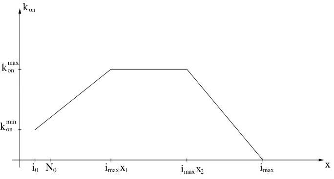
piecewise continuous formulation of the functionkon(x) given by the piecewise

linear representation (see Figure 2)

kon(x) =

                     kmin on +x

k_onmax−kmin_on

x1imax−i0 , x≤x1imax

kmaxon , x1imax≤x≤x2imax

kmax on −x

k_onmax

imax(1−x2), x2imax≤x≤imax

0, x≥imax.

In our numerical approximations, we chose i0 = 2, N0 = 500. The discrete

polymerization parameterskion,i=i0, .., N0, are then obtained as

ki_on:=kon(x=i).

We followed [52] in choosing to approximate kon by a function as depicted

in Figure 2. Other choices like a Gaussian bell curve are also possible (based on our discussions with S. Prigent, H. Rezaei and J. Torrent), but as we will subsequently conclude, the presently available data will not support estimation of parameters in these representations. Thus with this parametrization we have 5 more parameters, kmin_on , kmax_on , the fractions x1, x2, and imax, in addition to

the 4 basic parameters k_I+, k_I−, k_onN, kN_{of f} to be estimated using our data sets. That is,θ= (k+_I, k−_I, kN

on, kof fN , k min

on , kmaxon , x1, x2, imax) with scalar observations

f(t,θ)) =P

i≥i0ici(t).

The goal then in [53] was to estimate the 9 parametersk+_I, k−_I, kN

of f, kNon, and

kon (represented in parametrical form depicted in Figure 2 with the 5 additional

unknowns kmin

on , konmax, x1, x2, imax) that best fit the data. Equally important

(12)

x

k

on

k

on

k

on

max

min

i

max

i

max

x

2

i

max

x

1

N

0

i

0

Figure 2: Parametric representation forkon.

problemas well as a correct assumption on the measurement errors in the

in-verse problem. For this we use the ideas from residual plot analysis [17, 28] in attempts to obtain an acceptable statistical model as in equation (4).

3.5 Use of Residual Plots for Statistical Model Evaluation

To pursue a correct statistical model for the polymerized mass data, we carried out (as detailed in [13]) a series of inverse problems and residual plots with data set DS 4 of the experimental data collection. We first used DS 4 on the interval

t ∈ [0,8]. Based on some earlier calculations, we also chose the nucleation

indexi0 = 2 for all of our subsequent calculations. The residual plots given in

[13] strongly support the conclusions thatneitherof the initial assumptions for

statistical models and corresponding cost functionals (absolute error withγ= 0

and OLS or relative error withγ= 1 and IRWLS) are correct.

Based on these initial results and the speculation that early periods of the polymerization process may be somewhat stochastic in nature, we chose to sub-sequently use all the data sets on the intervals [t0,8] where t0 is the first time whenf(t0)>0.12 (thus larger than 12% of the non-dimensional total polymer-ized mass where it is supposed that the polymerization process becomes more

deterministic). Moreover, we used other values ofγbetween 0 and 1 to test data

set DS 4. Setting i0 = 2, we focused on the question of the most appropriate

values of γ to use in a generalized least squares approach (again see [17] for

further motivation and details). Analysis of the resulting residuals for random-ness suggested that eitherγ= 0.6 orγ= 0.7 might be satisfactory for use in a generalized least squares formulation.

(13)

problems for each of the 4 experimental data sets with initial concentration

c0 = 200 µmol and i0 = 2. We carried out the optimization over all data

points with f(tk) ≥ 0.12 and used the generalized least squares method with

γ= 0.6. The resulting graphics depicted in [13] again suggested thatγ= 0.6 is a reasonable value to use in any subsequent analysis of the polyglutamine data for inverse problem estimation and associated parameter uncertainty quantification.

3.6 Summary of Findings

In the problem outlined above, the authors of [13] (as did the authors of [52]) did indeed obtain a good fit of the curve and reasonable residuals . However,

they also found that the condition number of theκθ×κθ= 9×9 approximate

covariance matrixF =χT(θˆ)W(θˆ)χ(θˆ) is κ= 1024. Looking more closely at

the matrix F revealed a near linear dependence between certain rows, hence

the large condition number. One thus can readily draw thefollowing summary

conclusions:

1. One obtains a set of parameters for which the model fits well, but one

can-nothave any reasonable confidence in them using the asymptotic theories

from statistics, e.g., see the references [13, 52].

2. We suspect that it may not be possible to obtain sufficient information from our data set curves to estimate all 9 parameters with a high degree of confidence! This is based on our calculations with the corresponding covariance matrices as well our prior knowledge that the graphs depicted in Figure 1 are very similar to Logistic, Gompertz or other bounded growth curves. These curves can usually be sufficiently well-fit with parameterized models with at most 2 or 3 carefully chosen parameters!

To assist in the understanding of these issues, we turn to consider components of the associated sensitivity matrices

χ=

_∂f

∂θ

.

3.7 Sensitivity Analysis

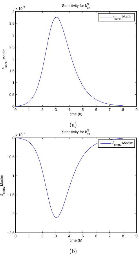
For the sensitivity analyses, we follow [17, 28] and carry out all computations using the differential system of sensitivity equations as detailed in those refer-ences. Our subsequent sensitivity analyses were carried out using data set DS 4

and the best estimateθˆobtained for this randomly chosen data set. As we see in

the figures below, the model is most sensitive to 4 parameters:k_I+, k−_I , kN on, kof fN .

The sensitivities for the remaining parameters are on the order of magnitude of 10−6 _{or less (e.g., see the plots in [13]). The observation} _f₍_t_;_θˆ_{) also exhibits}

some sensitivity with respect tox1. However, the parameterx1appears in the

(14)

ˆ

θ for the 9 best fit GLS parameters, i.e., θˆforκθ = 9. We note that since we

use the non-dimensional quantityf(t;θˆ) (or Madim) in the cost functionals, it is the sensitivity of this quantity with respect to the parametersθˆ(rather than any relative sensitivities), that will determine changes in the cost functionals to be minimized with respect to changes in the parameters.

0 1 2 3 4 5 6 7 8 9

−0.1 −0.09 −0.08 −0.07 −0.06 −0.05 −0.04 −0.03 −0.02 −0.01 0

time (h)

∂kIm

inus

Madim

Sensitivity for k_I−

∂_kIm_inus Madim

(a)

0 1 2 3 4 5 6 7 8 9

0 0.1 0.2 0.3 0.4 0.5 0.6 0.7

time (h)

∂kIplus

Madim

Sensitivity for k_I+

∂_kIplus Madim

(b)

(15)

0 1 2 3 4 5 6 7 8 9 0

0.5 1 1.5 2 2.5 3 3.5

4x 10

−5

time (h)

∂konN

Madim

Sensitivity for k

on N

∂_konN Madim

(a)

0 1 2 3 4 5 6 7 8 9

−2.5 −2 −1.5 −1 −0.5

0x 10

−3

time (h)

∂koffN

Madim

Sensitivity for k_offN

∂_koffN Madim

(b)

Figure 4: DS 4: Sensitivity off =M adimwith respect to(a)kN

(16)

3.8 Inverse Problems Motivated by Sensitivity Findings

Based on the sensitivity findings depicted above, we investigated a series of inverse problems in which we attempted to estimate an increasing number of parameters beginning first with the fundamental parametersk+_I andk_I−. In each of these inverse problems we attempted to establish uncertainty bounds for the estimated parameters using both the asymptotic theory and a generalized least squares version of bootstrapping described above in Section 2.4.

3.8.1 Estimation of k_I+ and k_I−

We first carried out estimation for the 2 parameters k+_I and k_I−. We use the

IRWLS formulation with γ = 0.6. Based on previous estimations with DS 4,

we fixed globally the parameter valueskN

on= 4616.962, kNof f = 93.332, k min on =

1684.381, kmax

on = 1.5152×109, x1= 0.0626, x2= 0.859, imax = 3.542×105.

In carrying out the inverse problem we used the initial guesses (again based

on previous estimations with DS 4) q0 _{for the parameters given by (}_k+

I)

0 ₌

2.16, (k_I−)0_{= 10}_._927.

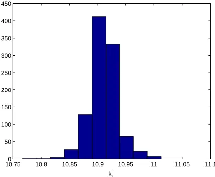
We also used the bootstrapping algorithm given above with M = 1000 to

compute means and standard errors. These are given in the table below and compare quite well with the asymptotic theory estimates. The corresponding bootstrapping distributions are depicted in Figures 5 and 6.

k+_I(boot)(GLS) k_I−(boot)(GLS) k_I+(asymp)(GLS) k−_I(asymp)(GLS)

mean 2.158 10.911 2.157 10.911

(17)

2.130 2.14 2.15 2.16 2.17 2.18 50

100 150 200 250 300 350 400 450

k

I +

Figure 5: DS 4: Two parameter estimation (k_I+,k_I−). Bootstrapping

distribu-tion fork+_I withM = 1000 runs.

10.750 10.8 10.85 10.9 10.95 11 11.05 11.1

50 100 150 200 250 300 350 400 450

k

I −

Figure 6: DS 4: Two parameter estimation (k_I+,k_I−). Bootstrapping

(18)

3.8.2 Estimation of 3 parameters

We tried next to estimate 3 parameters using the IRWLS formulation, again

with γ = 0.6. Once more we fixed all the parameters describing the domain

and the polymerization functionkon and we also fixed eitherkof fN ork N

on in the

corresponding inverse problems.

3.8.3 Estimation for k_I+, k_I− and kN on

We fixed values ofk_{of f}N , konmin, kmaxon , x1, x2, imax as before and used initial

values 2.1600, 10.9270, 4616.962 fork+_I, k−_I, kN

on, respectively.

We obtained the estimated parameters together with the corresponding

stan-dard errors, variances and the condition numbers κ of the corresponding

co-variance matrices for the 4 data sets as reported below. The resulting 95% confidence results based on the asymptotic theory were quite acceptable.

k_I+ k_I− k_onN SE σ2 κ

DS1 2.26 13.49 4616.96 (.012, .099,53.925) 8.52·10−6 ₈_.₈₉_·₁₀10 DS2 2.99 16.20 4616.96 (.021, .151,56.691) 9.67·10−6 ₄_.₃₇_·₁₀10 DS3 2.18 15.76 9840.31 (.011, .103,90.466) 6.45·10−6 ₃_.₉₄_·₁₀11 DS4 2.16 10.91 4616.96 (0.0089,0.0649,45.262) 6.36·10−6 ₇_.₁₄_·₁₀10

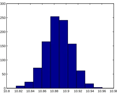
To compare these asymptotic results with bootstrapping, we carried out bootstrapping with data set DS 4 for the estimation of k+_I, k_I− and kNon with

the same initial values as above. We then obtained the following means and

standard errors (SE) for a run with M = 1000, which is compared to the

asymptotic theory in the table below.

k+_I(boot) k−_I(boot) kN

on(boot) k

+

I(asymp) k

−

I(asymp) k N

on(asymp)

mean 2.153 10.887 4616.962 2.157 10.910 4616.962

SE 0.0039 0.0219 0.00003 0.0089 0.0649 45.262

Of noticeable interest are the values obtained forkN

on and the bootstrapping

standard errors forkN

on which are extremely small. It should be noted that the

sensitivity of the model output with respect to kN

on is also very small. Thus

one might suspect that the iterations in the bootstrapping algorithm do not

change the values ofkN

on very much and hence one observes the extremely small

(19)

10.80 10.82 10.84 10.86 10.88 10.9 10.92 10.94 10.96 10.98 50

100 150 200 250 300

Figure 7: DS 4: Estimation fork_I+,k_I− andkonN: Bootstrapping distribution for

k_I− forM = 1000 runs.

2.140 2.145 2.15 2.155 2.16 2.165 2.17 50

100 150 200 250

Figure 8: DS 4: Estimation fork_I+,k_I− andkonN: Bootstrapping distribution for

(20)

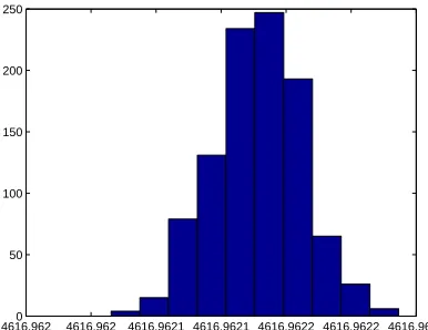
4616.9620 4616.962 4616.9621 4616.9621 4616.9622 4616.9622 4616.9623 50

100 150 200 250

Figure 9: DS 4: Estimation fork_I+,k_I− andkN

on: Bootstrapping distribution for

kN

(21)

3.8.4 Estimation for k_I+, k−_I and k_{of f}N

In another estimation, we fixed k_onN at 4616.962 along with the other fixed

parameter values used above and instead estimatedk_{of f}N along withk+_I andk−_I. Initial values for the 3 parameters were 2.16,10.9270, 108.256 fork_I+, k_I−, kN

of f,

respectively.

We obtained the estimated parameters and corresponding SE for the 4 data sets reported in tabular form below.

k+_I k−_I kN

of f SE σ2 κ

DS1 2.203 12.997 99.861 (.011, .091,1.208) 8.165·10−6 ₄_.₉₁₂_·₁₀7 DS2 2.893 15.474 100.019 (.019, .137,1.279) 9.323·10−6 ₂_.₄₈₆_·₁₀7 DS3 2.168 15.631 41.935 (.011, .102,0.424) 6.435·10−6 ₉_.₁₂₅_·₁₀6 DS4 2.181 11.090 90.536 (.009, .066,0.936) 6.289·10−6 ₃_.₀₄₃_·₁₀7

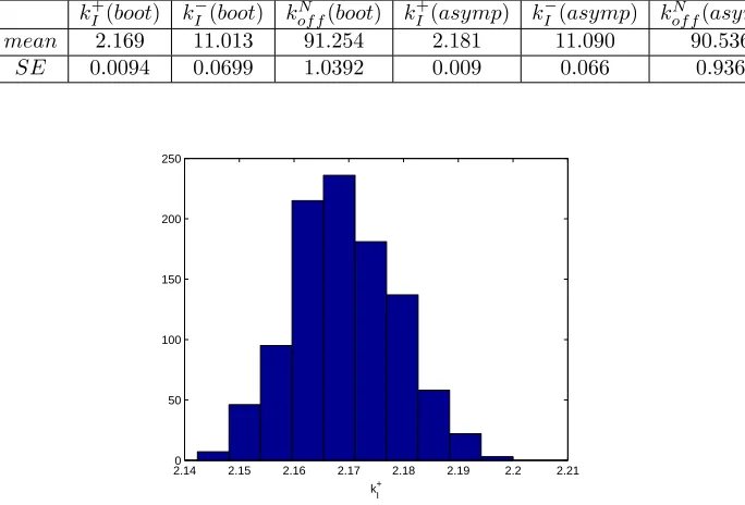
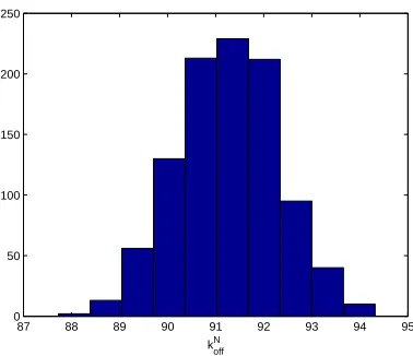
In addition, we carried out bootstrapping for DS 4. The bootstrapping

distributions fork+_I,k_I−andkN_{of f} are given in Figures 10-12. We then obtained

the following means and standard errors for a bootstrapping run withM = 1000

as compared to the asymptotic theory.

k+_I(boot) k−_I(boot) kN

of f(boot) k

+

I (asymp) k

−

I (asymp) k N

of f(asymp)

mean 2.169 11.013 91.254 2.181 11.090 90.536

SE 0.0094 0.0699 1.0392 0.009 0.066 0.936

2.140 2.15 2.16 2.17 2.18 2.19 2.2 2.21 50

100 150 200 250

k

I +

Figure 10: Three parameter estimation (k_I+,k−_I andkN

of f): Bootstrapping

(22)

10.80 10.9 11 11.1 11.2 11.3 50

100 150 200 250

k

I −

dis-tribution fork_I−,M = 1000 runs.

87 88 89 90 91 92 93 94 95

0 50 100 150 200 250

k

off N

dis-tribution forkN

(23)

3.8.5 Estimation of 4 main parameters

In light of the sensitivity analysis discussed above, we tried to estimate a combination of the parameters k+_I, k−_I, kN

on, kof fN (the parameter sets with

κθ = 4). From the original κθ = 9 parameter fits, parameters were fixed for

kmin

on , kmaxon , x1, x2, imax as 1684, 1.5×109, 0.062, 0.859, 3.5×105,

respec-tively. We obtained the following results for the estimation of the 4 parameters

using the data sets DS 1 to DS 4. In all of these results, the condition numberκ

of the Fisher’s Information Matrix is too large to carry out the required

inver-sion in order to compute standard errors. This,along with the sensitivity results

above, strongly supports the conclusion that the data sets do not contain suffi-cient information to estimate 4 or more parameters with any degree of certainty attached to the estimates. Again, this supports our expectation that the curves depicted in Figure 1 can each be readily and accurately modeled using simple growth models with at most 2 or 3 parameters. We will revisit this example and these conclusions after the next section where we introduce model comparison techniques as a tool in information content analysis.

k_I+ k_I− kN

on kNof f σ

2 _κ

(24)

4 Model Comparison: Nested Restraint Sets

Below we will demonstrate the use ofstatistically based model comparison tests

in several examples of practical interest. In these examples we are interested in questions related to information content of a particular given data set and whether the data will support a more detailed or sophisticated model to describe

it. In the next subsection we recall the fundamental statistical tests to be

employed here.

4.1 Statistical Comparison Tests

In general, assume we have an inverse problem for the model observationsf(t,θ)

and are givennobservations. As in (9), we define

Jn(Y;θ) =

n

X

i=1

wi(˜θ)−2γ(Yi−f(ti;θ))

2

(22)

where our statistical model has the form (4). Here, as before,θ0is the nominal

value ofθ which we assume to exist. We useΩ to represent the set of all the

admissible parametersθ. We make some further assumptions:

A5) Observations are taken at{tj}n

j=1 in [0, T]. There exists some finite mea-sureµon [0, T] such that

1 n

n

X

j=1

h(tj)−→

Z T

0

h(t)dµ(t)

asn→ ∞, for all continuous functionsh.

A6) J0(θ) = RT

0 (f(t;θ0)−f(t;θ))

2_dµ₍_t_{) =}_σ2_{has a unique minimizer in}_Ω_at

θ0.

Let Θn =Θn_{IRW LS}(Y) be the IRWLS estimator forJn _{as defined in (10)}

so that

Θn(Y) =argmin^

θ∈Ω

Jn(Y;θ)

and

ˆ

θn=argmin^

θ∈Ω

Jn(y;θ),

whereyis a realization for Y.

One can then establish a series of useful results (see [14, 17, 22] for detailed arguments and proofs).

Result 1: Under A1) to A6), 1

nΘ n₌ 1

nΘ n

IRW LS(Y)−→θ0asn→ ∞with probability 1.

(25)

A7) The nominal parameterθ0∈Rp satisfiesθ0∈int(Ω).

A8) f :Ω→C[0, T] is aC2 _function.

A10) J = ∂2J0

∂θ2 (θ0) is positive definite.

A11) ΩH = {θ ∈Ω|Hθ =c} where H is anr×pmatrix of full rank, and c

is a known constant. Here r is the number of constraints placed on the

reduced model parameters.

In many instances, including the motivating examples discussed here, one is

interested in using data to question whether the “nominal” parameterθ0 can

be found in a subsetΩH ⊂Ωwhich we assume for discussions here is defined by

the constraints of assumption A11). Thus, we want to test thenull hypothesis

H0: θ0 ∈ΩH, i.e., that the constrained model provides an adequate fit to the

data.

Define then

Θn_H(Y) =argmin^

θ∈ΩH

Jn(Y;θ)

and

ˆ

θnH =argmin^

θ∈ΩH

Jn(y;θ).

Observe thatJn₍_y_;_θˆn

H)≥Jn(y;θˆ n

). We define the related non-negative test statistics and their realizations, respectively, by

Tn(Y) =Jn(Y;θnH)−J

n₍_Y_;_θn₎

and

ˆ

Tn=Tn(y) =Jn(y;θˆ n H)−J

n₍_y_;_θ_ˆn₎_.

One can establish asymptotic convergence results for the test statisticsTn(Y)–

see [14]. These results can, in turn, be used to establish a fundamental result about much more useful statistics for model comparison. We define these statis-tics by

Un(Y) =

nTn(Y)

Jn₍_Y_;_θn₎, (23)

with corresponding realizations

ˆ

un=Un(y).

We then have the asymptotic result that is the basis of our analysis-of-variance–type tests:

Result 2: Under the assumptions A1)–A11) above and assuming the null

hypothesisH0 is true, then Un(Y) converges in distribution (asn→ ∞) to a

random variableU(r), i.e., Un

D

−→U(r), withU(r) having a chi-square distri-butionχ2₍_r_{) with}_r_{degrees of freedom.}

We note that if one is dealing with vector observations wheren=n1+n2is

(26)

last example in Section 6.4 , then asymptotic theory requires that bothn1→ ∞

and n2 → ∞. In any graph of a χ2 density there are two parameters (τ, α)

of interest. For a given valueτ, the value αis simply the probability that the

random variableU will take on a value greater thanτ. That is, Prob{U > τ}= αwhere in hypothesis testing,αis thesignificance level andτ is thethreshold.

We then wish to use this distribution Un ∼ χ2(r) to test the null

hypoth-esis, H0, that the restricted model provides an adequate fit to represent the

data. If the test statistic, ˆun > τ, then we reject H0 as false with confidence

level (1−α)100%. Otherwise, we do not reject H0. For our examples below,

we use aχ2_{(1) table, which can be found in any elementary statistics text or}

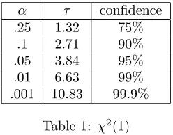
online. Typical confidence levels of interest are 75%,90%,95%,99% and 99.9% with corresponding (α, τ) values of (.25,1.32),(.1,2.71),(.05,3.84),(.01,6.63), and (.001,10.83), respectively.

α τ confidence

.25 1.32 75%

.1 2.71 90%

.05 3.84 95%

.01 6.63 99%

.001 10.83 99.9%

Table 1: χ2(1)

To test the null hypothesis H0, we choose a significance levelαand useχ2

tables to obtain the corresponding thresholdτ = τ(α) so that Prob{χ2₍_r₎ _>

τ} = α. We next compute ˆun = τ and compare it to τ. If ˆun > τ, then we

rejectH0 as false; otherwise, we do not reject the null hypothesisH0.

5 Model Comparison: Non-Nested Restraint Sets

There are a number of model comparison or model selection criteria in the statis-itival/mathematical literature that can be used to select a “best” approximating model from a prior collection of competing candidate models. These criteria are based on either hypothesis testing, e.g., log-likelihood ratio test, and residual sum of squares based model selection criterion such as the model comparison techniques for nested models as outlined in the previous section as well as infor-mation theory based techniques (e.g., the Akaike Inforinfor-mation Criterion as well as its variations [29, 30, 31, 47]). In these latter techniques the general goal in the model selection is to minimize both modeling error (bias) and estimation error (variance).

(27)

well-known measure of “distance” between two probability distribution models) and the maximum value of log-likelihood function of a given approximating model

(this relationship is referred to as the Akaike Information Criterion). These

criteria can be used to measure information lost when an approximating proba-bility distribution model is used to approximate the true probaproba-bility distribution

modelp0, which is tacitly assumed to exist for the model comparison/selection

techniques we describe here. That is, letp0denote the probability distribution

model that actually generates the data (that is, is the true probability density

function of some observationsY), andpbe a probability distribution model that

is presumed to approximate the data. In addition, pis assumed to be

depen-dent on a parameter vectorθ ∈_Rκθ _{(that is,}_p₍_·|_θ_{) is the specified probability}

density function of observationsY, and is used to approximate the true model

p0). Then the K-L information between these two models is given by

I(p0, p(·|θ)) = R

Ωyp0(y) ln

_p

0(y)

p(y|θ)

dy

= R

Ωyp0(y) ln(p0(y))dy− R

Ωyp0(y) ln(p(y|θ))dy,

(24)

where Ωydenotes the set of all possible values fory, and the second term in the

right side,R

Ωyp0(y) ln(p(y|θ))dy, is referred to as therelative K-L information.

5.1 A Large Sample

AIC

As we have noted, the AIC is based on K-L information theory, which measures the “distance” between two probability distribution models. In establishing the AIC, the maximum likelihood estimation method is used for parameter estima-tion. Note that the K-L informationI(p0, p(·|θM LE(Y))) is a random variable

(inherited from the fact that θM LE(Y) is a random vector). Hence, we need

to use the expected K-L information_EY(I(p0, p(·|θM LE(Y)))) to measure the

“distance” between a candidate distribution pand the assumed true

distribu-tionp0, whereEY denotes the expectation with respect to the true probability

density functionp0 of observationsY.

It was shown (e.g., see [32] for details) that for a large sample and “good”

model (a model that is close to p0 in the sense of having a small K-L value) we have

EYEX(ln(p(X|θM LE(Y))))≈ln(L(ˆθM LE|y))−κθ. (25)

Here ˆθM LE is the maximum likelihood estimate of θ given sample outcomes

y (that is, ˆθM LE =θM LE(y)),L(ˆθM LE|y) represents the likelihood of ˆθM LE

given sample outcomesy(that is,L(ˆθM LE|y) =p(y|ˆθM LE)), andκθis the total

number of estimated parameters (including mathematical model parametersq

and statistical model parameters). It is worth pointing out here that having a large sample and “good” model are used to ensure that the estimate ˆθM LE

provides a good approximation to some true valueθ0(involving the consistency

(28)

For historical reasons, Akaike multiplied (25) by −2 to obtain his criterion, which is given by

AIC=−2 lnL(ˆθM LE|y) + 2κθ. (26)

We note that the first term in theAICis a measure of the goodness-of-fit of the

approximating model, and the second term gives a measure of the complexity of the approximating model (i.e., the reliability of the parameter estimation of the model). Thus, we see that for the AIC the complexity of a model is viewed simply as the number of parameters in the model.

Based on the above discussion, we see that to use theAIC to select a best

approximating model from a given prior set of candidate models, we need to

calculate theAICvalue for each model in the set, and the “best” model is the

one with the minimumAICvalue. Note that the value of theAIC depends on

data, which implies that we may select a different best approximating model if

a different data set arising from the same experiment is used. Hence, theAIC

values must be calculated for all the models being compared by using thesame

data set. That is, theAICcannot be used to compare models for different data

sets. For example, if a model is fit to a data set with n = 140 observations,

one cannot validly compare it with another model when 7 outliers have been

deleted, leaving onlyn= 133.

Under reasonable assumptions (essentially normality of the measurement er-rors) [17, 18], one can use ordinary least squares (OLS), weighted least squares (WLS), or iterative reweighted weighted least squares (IRWLS) estimators in

place of the usual maximum likelihood estimators in formulatingAIC

compar-ison factors.

5.2 A Small Sample

AIC

The discussion in Section 5.1 reveals that one of the assumptions made in the

derivation of the AIC is that the sample size must be large. Hence, the AIC

may perform poorly if the sample sizenis small relative to the total number of

estimated parameters. It is suggested in [32] that theAIC can be used only if

the sample sizenis at least 40 times of total number of estimated parameters

(that is,n/κθ≥40). In this section, we introduce a small sampleAIC(denoted

byAICc) that can be used in the case whereN is small relative toκθ.

TheAICcwas originally proposed in [57] for a scalar linear regression model,

and then was extended in [47] for a scalar nonlinear regression model based on

asymptotic theory. In deriving theAICc, it was assumed in [47] that the

mea-surement errors Ej, j = 1,2, . . . , n, are independent and normally distributed

with mean zero and varianceσ2_{. In addition, the true model}_p

0was assumed to

be known with measurement errors being independent and normally distributed

with zero mean and varianceσ₀2. With these assumptions, the small sampleAIC

is given by

AICc=AIC+

2κθ(κθ+ 1)

n−κθ−1

, (27)

(29)

to as thebias-correction term. We observe that as the sample sizen→ ∞this bias-correction term approaches zero, and the resultant criterion is just the

usual AIC. From the remarks in the previous section and the results of [18],

we again note that one can equivalently use OLS, WLS, etc. estimators in the

formulation of theAICc model comparison terms.

It should be noted that the bias-correction term in (27) changes if a dif-ferent probability distribution (e.g., exponential, Poisson) is assumed for the

measurement errors. However, it was suggested in [32] that in practice AICc

given by (27) is generally suitable unless the underlying probability distribution is extremely non-normal, especially in terms of being strongly skewed.

TheAICc in the multivariate observation case was derived in [29] and

dis-cussed more fully in [32, 17].

5.3 Akaike Weights and the Selected “Best” Model

As we have noted above, the selected “best” model is the one with the minimum

AIC value. It should be noted that the selected model is specific to the set of

candidate models. It is also specific to the given data set. In other words, if one has a different set of experimental data arising even from the same experiment, one may select a different model. Hence, in practice, the absolute size of the

AIC value may have limited use in supporting the chosen best approximating

model. In addition, theAIC value is an estimate of the expected relative K-L

information (hence, the actual value of theAICis meaningless). Thus, one may

often employ other related values such as the Akaike difference and the Akaike weights.

The Akaike difference is defined by

∆i=AICi−AICmin, i= 1,2, . . . l, (28)

whereAICi is theAIC value of theith model in the set, andAICmin denotes

theAICvalue for the best model in the set, andlis the total number of models

in the candidate set for comparison. We see that the selected model is the one with zero Akaike difference. The larger ∆i, the less plausible it is that the ith

model is the best approximating model given the data set. Akaike weights are defined by

wi=

exp(−1 2∆i) Pl

r=1exp(− 1 2∆r)

, i= 1,2, . . . l. (29)

We note that the weights of all candidate models sum to 1, so the weight gives a probability that each model is the best model. Furthermore, the evidence ratio

wi(AIC)

wj(AIC)

(30)

indicates how much more likely modeli is compared to model j. In addition,

(30)

largest weights respectively, then the normalized probability

wi(AIC)

wi(AIC) +wj(AIC)

(31)

indicates the probability of modeliover modelj [61].

The Akaike weightwi is similar to the relative frequency for theith model

selected as the best approximating model by using the bootstrapping method. It can also be interpreted (in a Bayesian framework) as the actual posterior

probability that ith model is the best approximating model given the data.

We refer the interested reader to [32, Section 2.13] for details. Akaike weights

are also used as a heuristic way to construct the 95% confidence set for the

selected model by summing the Akaike weights from largest to smallest until

the sum is ≥0.95. The corresponding subset of models is the confidence set

for the selected model. Interested readers can refer to [32] for other heuristic approaches for construction of the confidence set.

As a followup to the weighting factors explanations construction of confi-dence sets, we emphasize that information criterion analysis is not a “test”, so one should avoid use of “significant” and “not significant”, or “rejected” and “not rejected” in reporting results. That is, null hypothesis testing should not be mixed with information criterion in reporting the results. In particular, one

should not use the AIC to rank models in the set and then test whether the

best model is “significantly better” than the second-best model.

6 Model Comparison and Information Content

Examples

In the first example we return to the polymerization example of Section 3 to illustrate use these model comparison techniques as interrogating tools for data set content. We discuss these in the context of nested models as well as report

onAIC comparison factors. In a second example we compare fits for several

different models to describe simple decay in a size histogram for aggregates in amyloid fibril formation; this example is also related to aggregate formulation discussed in Section 3. In a related example we consider population experiments

with green algae, formally known asRaphidocelis subcapitata. In [10, 18] efforts

by the authors were concerned with the growth dynamics of the algae as this

is the major food source forDaphnia magna [2] in experimental settings. In a

fourth example we investigate whether the information content in data sets for the pestLygus hesperus in cotton fields as it is currently collected is sufficient to support a model in which one distinguishes between nymphs and adults.

6.1 Polymerization (again!)

(31)

statistically significantly improved model fit (we again use DS 4 for y). Our

null hypothesis in each case is: H0: The restricted or constrained model is

ade-quate (i.e., the fit-to-data is not significantly improved with the model contain-ing the additional parameter as a parameter to be estimated). We summarize our findings using the model comparison tests.

A) The model with estimation of{k_I+, k_I−}holding the other parameters fixed was compared with the model with estimation of{k+_I, k−_I, kN_{of f}}. We found (in each case here n=699),

Jn(y; ˆθnH) =.0044192109

,

Jn(y; ˆθn) =.0043709501

and ˆun = 7.7178. Thus, we reject H0 at a 99% confidence level. This

means that the data set does support at a statistically significant level

the model with estimation of the additional parameter kN_{of f}. Note that

if we compute the correspondingAIC comparison factors (again n=699),

we obtain AIC =−8362.04 for the two parameter model versus AIC =

−8367.72 for the three parameter model. This difference suggests the

estimation of 3 parameters yields a better model fit.

B) The model with estimation of{k_I+, k_I−}vs. the model with estimation of

{k_I+, k_I−, kN

on} was compared. We find

Jn(y; ˆθn) =.0044192108

with ˆun = 7.49×10−06.Thus we cannot rejectH0at any reasonable

con-fidence level so that estimation of the additional parameterkN

oncannot be

supported at any meaningful positive statistical level. The corresponding

AIC factors are both -8360.04 which offers no support for estimation of

the additional parameter.

C) The model with estimation of{k+_I, k−_I, kN

of f}was compared with the model

with estimation of {k+_I, k_I−, kN of f, k

N

on}. To the order of computation

ac-curacy we found no difference in the cost functions (hence no difference

in theAIC factors) in this case and therefore we do not rejectH0 at any

reasonable confidence level.

D) The model with estimation of{k_I+, k_I−, kN

on}vs. the model with estimation

of{k_I+, k_I−, kN

on, kNof f} was compared. We found

Jn(y; ˆθnH) =.0044192108

and

Jn(y; ˆθn) =.0043709780

with ˆun= 7.7133 and hence we rejectH0 with a confidence level of 99%.

The corresponding AIC factors are -8360.04 and -8365.71, respectively,

(32)

From these and the preceding results from Section 3, we conclude that the information content of the typical data set for the dynamics considered in the nucleated polymerization models above will support at most 3 parameters

{k+_I, k−_I, kN_{of f}} estimated with reasonable confidence levels.

6.2 Size distributions of aggregates in amyloid fibril

for-mation

In a recent paper [53], a question was addressed about size distribution of aggre-gates in amyloid fibril formation. While an exponential distribution was shown to provide a reasonable fit to the data depicted in Figure 13, the question arose as to whether another distribution such as the Weibull, Gamma, or some other decay distribution with more parameters might provide a better fit.

6.2.1 The Exponential, Weibull, Gamma and other Decay Distribu-tions

On initial observation, the data appears to be well suited to an exponential distribution. The exponential distribution probability density function is defined asE(x;λ) =λe−λx_{. Note that when fitting the data, an additional parameter}

Awas added to the exponential function resulting in a total of two parameters

and the function to be defined for these purposes as

E(x;A, λ) =Aλe−λx.

The Weibull distribution probability density function [6, 62] is defined as (for the purposes of modeling the data we again add the additional parameter A)

W(x;A, λ, k) =Akλ(λx)k−1e−(λx)k, x≥0.

Note that if we take k = 1 we have that W(x;A, λ,1) = E(x;A, λ). This

function is shown plotted in [6, 62] with several values of k. One can see that

whenk= 2 ork= 1 the function also bears a resemblance to the shape of our

data.

The probability density function of the Gamma distribution is defined as

[6, 45] (we again include the additional parameterA for modeling purposes)

G(x;A, k, λ) =A λ

k

Γ(k)x

k−1_e−λx _for_{x >}_{0 and}_{k, λ >}₀_,

where Γ(k) is the Gamma function evaluated at k. One can see [6, 45] that

whenk= 1 and λ= 0.5, the Gamma probability density function again has a

similar shape to the data. Since we know that Γ(1) = 1, we can see that when we takek= 1 we have thatG(x;A,1, λ) =E(x;A, λ).

The two final models we consider are the logistic decay model,

(33)

and the Gompertz decay model [49],

D(x;A, λ, k) =Aexp (−λe−kx). (33)

The exponential model has only two parameters which must be estimated while each of the other models involve three parameters. In the fits-to-data depicted in Figure 13, we see that all 5 functions provide reasonable fits to the data. Thus an interesting first question is whether we can obtain a statistically significantly better fit to the data by allowing an additional third free parameter

kin either the Weibull or Gamma distribution in comparison to the 2 parameter

(A, λ) exponential model. We further consider two additional decay models, the

logistic and the Gompertz for which the nested model comparison techniques

are not applicable. We thus turn to theAICc factors for comparisons ranking

for all five models.

size of fibril

0 0.1 0.2 0.3 0.4 0.5 0.6

proportion of observed fibrils

0 0.02 0.04 0.06 0.08 0.1 0.12 0.14 0.16

0.18 Fibril Data with Fitted Functions

Exponential Distribution Model Fit; AIC_c: -227.7032; w = 0.13751

Weibull Distribution Model Fit; AIC

c: -228.973; w = 0.25947

Gamma Distribution Model Fit; AIC

c: -229.0949; w = 0.27577

Logistic Decay Model Fit; AIC

c: -228.3886; w = 0.19371

Gompertz Decay Model Fit; AIC

c: -227.6445; w = 0.13354

Data

Figure 13: This figure depicts experimental data (n= 27) along with the fitted

models as indicated. For each model theAICc and the model weights are also

given.

6.2.2 Results using the comparison tests

We carried out fits-to-data using an OLS version of the inverse problems (we

established with preliminary computations and residual analysis that γ = 0

(34)

and alternative hypothesis for 2 of the alternative models (a Weibull and a Gamma distribution) as compared to the exponential:

• H0: The fit provided by an alternative model is not statistically

signifi-cantly different from the fit with an exponential distribution.

• HA: The alternative model with an unrestricted additional parameter k

provides a statistically significantly better fit than the exponential model

(corresponding to the restrictionk= 1).

When comparing the best fits of the exponential (e) vs. the Weibull (W) distributions we obtained the following results:

J_nW = 1.4359×10−4,

and

J_ne= 1.6081×10−4,

with

ˆ

T_neW = 4.6495×10−4,

and

ˆ

ueW_n = ¯τ = 3.2381

for the exponential-Weibull (eW) comparison test statistic. In this case we

cannot reject the null hypothesis at the 95% or higher level. We can rejectH0

at the 90% confidence level. The correspondingAICcfactors are given in Table

2 below and fully support these findings.

When comparing the best fits of the exponential (e) vs. the Gamma (G) distribution, we obtained the following results:

JnG= 1.4277×10−4,

and

J_ne= 1.6081×10−4,

with

ˆ

T_neG= 4.8693×10−4,

and

ˆ

ueG_n = ¯τ= 3.4105

for the exponential-Gamma (eG) comparison test statistic. Again in this case we cannot reject the null hypothesis at the 95% or higher level but we can reject

H0at the 90% confidence level. The correspondingAICcfactors given in Table

2 below again fully support these findings.

Using a threshold of α= 0.05, we fail to reject the null hypothesis H0 in

(35)

Model AICOLSc wi

Exponential -227.70 0.138

Weibull -228.97 0.259

Gamma -229.09 0.276

Logistic -228.39 0.194

Gompertz -227.64 0.134

Table 2: Comparison ofAICc values for each candidate model for the fibril size

data

6.2.3 Results using AICc factors

We next considered additional model fits involving Gompertz and logistic

distri-butions and computed the correspondingAICcfactors. As indicated in Table 2,

the Gamma distribution model is considered the ’best’ of the candidate models for this data, closely followed by the Weibull model. However, using the evidence ratio in equation (30), the Gamma model is only 1.1 times more likely to be the best model in terms of Kullback-Leibler discrepancy than the Weibull model with a normalized probability of 0.52 (using equation (31) ) when compared to the Weibull model. However, when comparing the normalized probability of the Gamma distribution model to the worst model out of the candidate models (the exponential distribution model), there is a 0.68 probability of the Gamma dis-tribution model as the preferred model over the exponential disdis-tribution model.

6.3 Growth dynamics for green algae

Raphidocelis

sub-capitata

In ecology, daphnia (e.g.,D. magna) can be used as early warning organisms

be-cause of changes in the daphnia population dynamics (thus they can be thought of as the modern day “canary in the mine shaft”) in response to changing dy-namics in the environment. The authors of [10] were concerned with the growth

dynamics of the algae as this is the major feeding source forDaphnia magna [2]

in experimental settings. In a recent paper [10] longitudinal data were collected from four replicate population experiments with green algae, formally known as Raphidocelis subcapitata, and analyzed for growth. Here we compare three different dynamical population models for algae growth: the classical logistic model, the Bernoulli model, and the Gompertz model. In doing this we use

here both the model comparison and the AICc methodology outlined above.

The logistic model is a special case of the Bernoulli whereas the Gompertz is not directly related to either of the other two.

The logistic model is given by

dx

dt =rx(t)

1−x(t)

K

, x(0) =x0 (34)

(36)

The Bernoulli model contains one additional parameterβ and is given by

dx

dt =rx(t) 1− _x₍_t₎

K

β!

, x(0) =x0.

Note that the logistic growth model is obtained from the Bernoulli growth model

by settingβ equal to 1. In standard form, the parametersK andβ are found

jointly in the denominator, possibly causing a problem with identifiability. To

address this issue, we let ˆK=Kβ and instead consider the model

dx(t)

dt =rx(t)

1−(x(t)) β

ˆ K

, x(0) =x0, (35)

where K can be obtained from ˆK using K = ˆK(1/β)_{. The third model we}

consider is the Gompertz model,

dx(t)

dt =κx(t) log

_K

x(t)

, x(0) =x0, (36)

where K is the carrying capacity as in the other two models and κscales the

time. We note that both the logistic and Gompertz models contain only two

(κq = 2) model parameters while the Bernoulli model contains three (κq= 3)

model parameters, where in the notation of Section 5.2, we have θ = [q, σ]T

andκθ=κq+ 1.

In terms of modeling the algae data, it is demonstrated in the paper by Banks et al. [10] that the appropriate statistical model for this data is a parameter

dependent weighted error statistical model withγ= 1 in Equation (6). Thus we

useγ= 1 and the GLS (i.e., IRWLS) in computing our minimization result. In

Table 3 we present comparison results for the logistic model for each replicate

vs. the Bernoulli model with J_Bern = .5857416 for each replicate. From this

table we can conclude from the comparison tests that the Bernoulli model is preferable at all reasonable confidence levels over the logistic model.

Replicate 1 Replicate 2 Replicate 3 Replicate 4

Model Jn

log Jlogn Jlogn Jlogn

logistic 1.024769 1.36611 1.368 1.951

ˆ

un _26.92 _47.88 _48.22 _83.79

Table 3: Comparison of model fit cost valuesJn

logand corresponding ˆun for each

logistic vs. Bernoulli withJ_Bern =.5857416 for the algae data

As this was a small data set with only n = 36 data points for each of the

(37)

is,

AICIRW LS≈nln



  

n

P

j=1

w_j−2(yj−f(tj,ˆqMW LS))

2

n



  

+ 2(κq+ 1), (37)

wherewj = ˆwjM ≈fγ(tj; ˆqIRW LS) whereM is the number of times the process

is enumerated in the IRWLS alogrithm of Section 2.2 andκθ =κq+ 1. Thus

we use here

AICIRW LSc= AICIRW LS+

2(κq+ 1) (κq+ 2) n−κq

. (38)

The results for each replicate are given in Table 4 with the fitted models and data fits for replicate 1 plotted in Figure 14. As shown in Table 4, there is minimal difference across the four replicates and in each case, the smallest AIC value is given by the Gompertz model followed closely by the Bernoulli model. Recall that the Gompertz model has 2 parameters; whereas the Bernoulli model has three; therefore, although the two curves are lying on top of one another in Figure 14, the Bernoulli model is penalized more by the extra parameter. If we heuristically compare the Gompertz and Bernoulli models using the evidence ratio in equation (30) and the normalized probability in equation (31), we see that the Gompertz model is only 1.03 times more likely with a normalized probability of only 0.51 (only slightly more than equal probability). Therefore, either the Gompertz or the Bernoulli model appears to be a good model of the candidate models examined.

Replicate 1 Replicate 2

Model AICIRW LSc wi AICIRW LSc wi

logistic -127.42 2.7e-05 -117.07 1.5e-07

Bernoulli -147.05 0.492 -147.05 0.492

Gompertz -147.11 0.508 -147.11 0.508

Replicate 3 Replicate 4

Model AICIRW LSc wi AICIRW LSc wi

logistic -117.02 1.5e-07 -104.24 2.5e-10

Bernoulli -147.05 0.492 -147.05 0.492

Gompertz -147.11 0.508 -147.11 0.508

Table 4: Comparison of AICIRW LScvalues and weights for each candidate model

(38)

time

0 50 100 150 200 250 300 350 400 450

algae count

0 1000 2000 3000 4000 5000

6000 Algae Data with Fitted Functions

Logistic Growth Model Fit; AIC_c: -127.4247; w = 2.6923e-05 Bernoulli Growth Model Fit; AICc: -147.0514; w = 0.49206

Gompertz Growth Model Fit; AIC_c: -147.1148; w = 0.50791 Data

Figure 14: This figure graphs experimental algae data along with the fitted

models given by equations (34) - (36). For each model, the AICc (equation

(38)) and the model weight (equation (29)) are given.

6.4 Lygus hesperus

Population Dynamics: Importance of

Nymph Deaths

Our next example concerns the methodology for insect counting and revolves around the question of how detailed field counts need to be in environmental studies. In particular, in labor intensive efforts to track pests in field environ-ments, is it necessary to keep track of nymph mortality? We investigate this

question in the context of monitoring of Lygus hesperus, a prevalent insect in

California which feeds on cotton and other plants [40]. Given a robust data

set of L. hesperus counts from over 500 Californian fields over several years,

we hope to provide more information about theL. hesperus and direct future

research relating to its effects on crops. But first we hope to inform the data collection process carried out by farmers and their associates. We propose 2 ordinary differential equation models, one of which features nymph mortality, estimate parameters for each model, and perform model comparison techniques to determine which model is more appropriate, given the population dynamics and the nature of the data.

Our main database consists of over 1500 data sets (comprising over 500

distinct fields) of L. hesperus counts. One data set is characterized by the

following: a designated pesticide control advisor (PCA) counts the number of