| INVESTIGATION
A Uni
fi
ed Characterization of Population Structure
and Relatedness
Bruce S. Weir*,1and Jérôme Goudet†,‡
*Department of Biostatistics, University of Washington, Seattle, Washington 98195,†Department of Ecology and Evolution and ‡Swiss Institute of Bioinformatics, University of Lausanne, 1015 Switzerland ORCID IDs: 0000-0002-4883-1247 (B.S.W.); 0000-0002-5318-7601 (J.G.)
ABSTRACTMany population genetic activities, ranging from evolutionary studies to association mapping, to forensic identification, rely on appropriate estimates of population structure or relatedness. All applications require recognition that quantities with an underlying meaning of allelic dependence are not defined in an absolute sense, but instead are made“relative to”some set of alleles other than the target set. The 1984 Weir and Cockerham FST estimate made explicit that the reference set of alleles was across
populations, whereas standard kinship estimates do not make the reference explicit. Weir and Cockerham stated that their FST
estimates were for independent populations, and standard kinship estimates have an implicit assumption that pairs of individuals in a study sample, other than the target pair, are unrelated or are not inbred. However, populations lose independence when there is migration between them, and dependencies between pairs of individuals in a population exist for more than one target pair. We have therefore recast our treatments of population structure, relatedness, and inbreeding to make explicit that the parameters of interest involve the differences in degrees of allelic dependence between the target and the reference sets of alleles, and so can be negative. We take the reference set to be the population from which study individuals have been sampled. We provide simple moment estimates of these parameters, phrased in terms of allelic matching within and between individuals for relatedness and inbreeding, or within and between populations for population structure. A multi-level hierarchy of alleles within individuals, alleles between individuals within populations, and alleles between populations, allows a unified treatment of relatedness and population structure. We expect our new measures to have a wide range of applications, but we note that their estimates are sensitive to rare or private variants: some population-characterization applications suggest exploiting those sensitivities, whereas estimation of relatedness may best use all genetic markers withoutfiltering on minor allele frequency.
KEYWORDSallele matching; correlation of alleles;FST; identity by descent; rare variants
W
E offer here a unified treatment of relatedness and population structure with an underlying framework of allelic dependence, where the degree of dependence can be quantified as the probability the alleles are identical by de-scent (ibd) or as the correlation of allelic-state indicators. We follow Thompson (2013) in regarding ibd for a set of alleles as being relative to some other, reference, set:“There is noabsolute measure of ibd: ibd is always relative to some refer-ence population.” In other words, ibd implies a reference point, and ibd status for different alleles at this point is often implicitly assumed to be zero. The need for a reference set for allelic-state correlations was made explicitly by Wright (1951): “the correlation between random gametes, drawn from the same subpopulation, relative to the total, is given by . . .” (emphasis added), and for inbreeding by Wright (1943):“The inbreeding coefficient is zero relative to the unit groups,Firelative to the intermediate groups andFtrelative to the total.”
A function of allelic dependence of particular interest to us is FST;which we will show below can be expressed as the probability of ibd of pairs of alleles within populations rela-tive to that for pairs of alleles from different populations. The Copyright © 2017 by the Genetics Society of America
doi:https://doi.org/10.1534/genetics.116.198424
Manuscript received November 17, 2016; accepted for publication May 17, 2017; published Early Online May 26, 2017.
Available freely online through the author-supported open access option.
uses of estimates of this quantity are widespread, and here we note, for instance, a recent discussion by McTavish and Hillis (2015) who used “pairwise FST for all pairs of populations using Weir and Cockerham’s method.”We suggest that a more informative analysis may result from our population-specificFST estimates (Weir and Hill 2002; Weiret al.2005; Browning and Weir 2010). Other authors (e.g., Balding and Nichols 1995; Beaumont and Balding 2004; Shriver et al. 2004; Gaggiotti and Foll 2010) have also discussed the advantages of working with population-specificFST values instead of single values for a set of populations, or of values for each pair of populations, and our recognition of allele frequency correlations among pop-ulations extends their work. Interpopulation correlations have also been considered by Fuet al.(2003), and in the Bayesian treatments of Fuet al.(2005), Songet al.(2006), Karhunen and Ovaskainen (2012) and Günther and Coop (2013). Here we allow for correlations in providing explicit moment estimates that apply to both populations and individuals.
The usual globalFST measure can be regarded as an un-weighted average of population-specific values, and, because it is an average, it masks the variation among populations that can indicate the effects of past selection (Beaumont and Balding 2004; Weir et al.2005). The global measure can diminish signals of population history, and this diminu-tion has become more pronounced as genetic marker data have become richer, and real differences among populations have become more evident.
As Astle and Balding (2009) noted“population structure and [cryptic] relatedness are different aspects of a single con-founder: the unobserved pedigree defining the (often distant) relationships among the study subjects.”A similar point was made by Kanget al.(2010):“The presence of related individuals within a study sample results in sample structure, a term that encompasses population stratification and hidden relatedness.” Our goal is to provide a unified approach to characterizing population structure and individual relatedness and inbreeding, in terms of both the underlying parameters and the methods of estimation. By working with proportions of pairs of alleles that match, or are the same type, we can give a single estimator for FST;where the pairs are from the same or different populations, and for inbreeding or coancestry, where the pairs are from the target individual(s) or from all pairs of individuals in a study. Measures of population structure are seen to be averages of coancestry measures for individuals within those populations as has been noted by Karhunen and Ovaskainen (2012).
Ibd refers to the history of pairs of alleles, and a consider-ation of historical“genetic sampling”(Weir 1996) shows that ibd measures allow quantification of the variance of allele frequencies among evolutionary replicates of these histories. Data from a single population or a single individual have no information about this variance, and so do not allow estimation of ibd probabilities. We might regard multiple loci as providing replication of the genetic sampling process, or we might collect data from multiple populations. An exception is when allele frequencies and ibd status in the reference population are as-sumed known, as is implied for standard methods for estimating
relatedness and inbreeding (e.g., Ritland 1996; Purcell et al. 2007; Yang et al.2011; Wang 2014) or in forensic science if the frequencies are taken from databases (e.g., Balding 2003). If, instead, estimation methods make use of frequencies from a sample of individuals, they are providing estimates of the in-breeding or relatedness ibd measures relative to those measures for all individuals in the sample. This point was also made by Yu et al.(2006), who spoke of“adjusting the probability of identity by state between two individuals with the average probability of identity by state between random individuals”in order to ad-dress ibd. Existing relatedness estimation methods that do not use allele frequencies (e.g., KING-robust, Manichaikul et al. 2010) estimate ibd between individuals (coancestry) relative to that within individuals (inbreeding).
For both population structure and relatedness, we propose the use of allelic matching proportions within and between individuals or populations in order to characterize ibd for an individual or a population relative to a reference set of ibd values. We use allele matching, equivalent to homozygosity and complementary to heterozygosity as used by Nei (1973), rather than components of variance (Weir and Cockerham 1984: hereafter WC84). Although our matching proportions can be translated into the sums of squares used by WC84 we believe they may have more intuitive appeal. Our present treatment also differs from that in WC84 by using un-weighted averages of statistics over populations instead of the weighted averages that were more appropriate for the WC84 model of independent populations. We return to this aspect in theDiscussion.
The size of current genetic studies requires computation-ally feasible methods for estimating relatedness between all pairs of individuals, potentially 5 billion pairs for the TOPMed project (http://www.nhlbiwgs.org). The scale of the task may well rule out maximum likelihood approaches (e.g., Thompson 1975; Ritland 1996; Milligan 2003) and Bayesian methods (e.g., Gaggiotti and Foll 2010), and Karhunen and Ovaskainen (2012) have reviewed the challenges of selecting the allele frequency distributions needed for likelihood- and Bayesian-based methods. Moment estimates seem still to be relevant, therefore, and will be presented here.
Materials and Methods
Allele-pair dependencies
the situation when they are not, as have others (e.g., Holsinger et al. 2002). We write the dosageXu of allele u for a diploid individual as the sum of thex’s for the two alleles carried by the individual, and for haploids the dosage is Xu ¼xu:For SNPs, we writeXas the dosage of the reference allele.
We stipulate that the expected value ofxu;where expec-tation is over replicates of the evolutionary history of that allele, ispu;the probability a random allele is of typeu, re-gardless of which individual carries that allele or which pop-ulation contains that individual. The essence of our treatment rests on the expectation of the products of twoxu’s, or the probabilities that pairs of alleles are both of typeu. For alleles AandA9;with indicatorsxuandx9u;we stipulate the expec-tation to be
Exux9u
¼p2
uþpu
12pu
u: (1)
As ℰðx2
uÞ is also pu; we see that the variance of xu is
puð12puÞ for any allele at the locus of interest. We also see, from Equation 1, that the covariance of xu and x9u is
puð12puÞu;and it follows that the quantityuis the correla-tion of the indicators for pairs of alleles as in the writing of Cockerham (e.g., Cockerham 1969). There is no requirement in Equation 1 foruto be positive, and, for example, negative values are expected for the two alleles carried by one indi-vidual in populations for which there is avoidance of mating between relatives. We add individual and population identi-fiers touin Table 1.
Following the work of Malécot (see review by Epperson 1999), we can also interpret Equation 1 withudefined as the probability that allelesA;A9are ibd. It is then the case thatu cannot be negative. Either of the two alleles has probability
pu of being of type u. The other allele has probabilityuof being ibd to the first, and so is also of type u, and it has probabilityð12uÞof not being ibd to thefirst, and so is of type uwith probabilitypu:If we follow Thompson (2013),
and regard ibd alleles as those that descend from a single allele in a reference population, the allele probability pu refers to the reference population. We distinguish the expected value pu from the actual allele frequency pu in a population, and from the frequency ~pu in a sample from the population, as listed in Table 1.
We will phrase much of our subsequent discussion in terms of ibd probabilities, but will return to the allelic indicator correlations on occasion. Our estimation procedures rest on Equation 1 and so will hold for both interpretations. We turn first, however, to some predictions of ibd probabilities. Predicted ibd probabilities
Individuals:For a single diploid individualj, the inbreeding coefficientFj is the probability its two alleles are ibd. The coancestry, or kinship, coefficient ujj9 for individuals j;j9 is
defined here as the average of the four ibd probabilities for one allele from each individual. It follows that the coan-cestry of individual j with itself is ð1þFjÞ=2: Generally, however, we will follow WC84 and reserve the term coan-cestry for distinct individuals. For haploids, inbreeding coefficients are not needed, and kinship is the ibd proba-bility of the allele in individualjwith the allele in individ-ual j9:We will have occasion to use uS;the average over pairs of individuals of the coancestries for (samples from) a population. In Table 1, we have added superscripts to indicate the populations from which the individuals are drawn.
If diploid individualJis ancestral to bothjandj9;and if there are n individuals in the pedigree path joiningj to j9 through J, including j and j9; then ujj9¼Pð0:5Þnð1þFJÞ;
where FJ is the inbreeding coefficient of J, and the sum is over all ancestors J and all paths joiningj to j9through J (Wright 1922). The coancestryujj9is also the inbreeding
co-efficient for an individual with parentsj;j9:If ancestorJ is further back in time than the reference time, then it does not contribute to the relatedness of individualsjandj9:
Table 1 Notation
Quantity Notation
Allele Ai
jkfor allelek2 f1;2g;individualj2 f1;2;. . .:nig;populationi2 f1;2;. . .rg Allelic indicator xijkufor alleleAijkbeing of typeu
Allele frequency puexpected value ofxijkufor alli;j;k
piuactual frequency for allele typeuin populationi ~
piuobserved frequency for allele typeuin sample from populationi
Theta uiijk9;j9k9is probability of ibd between allelekin individualjfrom populationiand allelek9in individualj9from populationi9 Inbreeding coefficient Fijis the ibd probability for the two alleles for individualjin populationi:Fji¼1
2
P2
k¼1
P2
k9¼1;k96¼kuiijk;jk9 Coancestry coefficient Coancestryujji9is the ibd probability for a pair of alleles drawn from individualsj;j9in populationi:
ui jj9¼14
P2
k¼1
P2
k9¼1uiijk;j9k9:uSiis the average ofuijj9for all pairsj;j9:uSis the average over populations ofuSi:For any two distinct alleles drawn from populationi, the ibd probability isui
W:The average over populations ofuWi isuW:uBis the average of ibd probabilities for alleles from different populations
Relative inbreeding The relative inbreeding coefficient for individualjin populationiisbi
j¼ ðFji2uRÞ=ð12uRÞ:referenceuRisuiSoruB Relative coancestry The relative coancestry coefficient for individualsj;j9in populationiisbi
jj9¼ ðuijj92uRÞ=ð12uRÞ:referenceuRisuiSoruB Population-specificFST bi
WT¼ ðuiW2uBÞ=ð12uBÞis probability two alleles drawn from populationiare ibd, relative to the probability an allele drawn from one population is ibd to an allele drawn from another population.bi
Populations:For a single population, the average coancestry coefficientuSwill refer to pairs of distinct alleles, one in each of two distinct individuals. For populations in which there is random union of gametesFj¼ujj9for alljandj96¼janduwill
refer to a random pair of distinct alleles in the population regardless of the individuals in which they are carried. If we wish to distinguish this allele-based quantity from genotype-baseduS;as we do below, then we write it asuW:In Table 1, we show superscripts to denote population, and we adopt that convention now to describe the accrual of ibd in random-mating population i with constant population size Ni:Without mutation,ui[uiW values fortdiscrete genera-tions after the time when the population had ibd probability
uið
0Þ;satisfy
uiðtÞ¼1212uið0Þ12 1 2Ni
t
: (2)
This result was discussed by Wright (1931), although not quite in this form, withuið0Þshown explicitly. We plotufrom Equation 2 in thefirst row of Figure 1.
As for pairs of individuals, the coancestry for pairs of populations is defined here as the average ibd probability for pairs of alleles, one in each population. For populationsi;i9 the quantityuiiB9is the average over all such pairs of alleles and it does not matter whether or not there is random mating within each population. If there is random mating within each of two populations i¼1;2 with constant population sizesN1;N2;however, then genetic drift in thetdistinct gen-erations since they diverged from a common ancestral pop-ulation whereu12ð0Þwas the ibd probability provides
uiðtÞ¼1212u12ð0Þ12 1 2Ni
t
; i¼1;2:
u12ðtÞ¼u12ð0Þ
In the absence of mutation and migration, the between-population ibd probabilityu12ðtÞat present timetis the same as it was, u12ð0Þ; in the common ancestral population. To avoid having to specify the ancestral valueu12ð0Þ;we define the relative coancestries within populations as biðtÞ ¼ ½uiðtÞ2u12ðtÞ½12u12ðtÞ for i¼1;2: It is pairs of alleles,
Figure 1 Effects of Drift, Muta-tion and MigraMuta-tion onuandbas a function of generation. For all pan-els, N1¼10;000 andN2¼100:
Left column (A, C, E) u1in red,
u2 in blue, u12 in orange. Right
column (B, D, F)b1
WTin red,b2WT
in blue,bWTin orange. (A, B) Drift
only (no mutation nor migration).
u1;u2 and b tend to 1, u12¼
0:000:(C, D) Drift and Mutation
m¼1023;m1¼m2¼0: u and
bhave positive limits,1. At equi-librium, u1¼0:024;u2¼0:714;
u12¼0:000;b1
WT¼0:024;b2WT¼
0:714;bWT¼0:369:(E, F) Drift,
Mutation and Migration. m¼
1023;m1¼1022;m2¼0:u
pos-itive and,1,bWTis positive but
b1
WT is negative. At equilibrium,
u1¼0:543;u2¼0:714; u1 2¼
0:596; b1
W T¼20:131; b2W T¼
one from each of populations 1 and 2, that serve as a refer-ence for describing the ibd status for alleles within each of populations 1 and 2, and there is zero ibd between the two populations relative to this reference. For a study in which there are only these two populations, we write
uW¼ ðu1þu2Þ=
2 and bW¼ ðb1þb2Þ=2: We also write
uB¼u12;
and we could writebB¼ ðuB2u12Þ=ð12u12Þ but this is zero for two populations.
For a set ofrpopulations, we make use of the average over populations of the between-individual, within-population, coancestries, uS¼Pr
i¼1uiS=r; and the average over pairs of populations of the population-pair coancestries, uB¼
Pr
i¼1Pri9¼1;i96¼iuiiB9=½rðr21Þ:We now have two possible refer-ence sets for within-population coancestries. Relative to all pairs of individuals in populationi, the coancestry for indi-viduals j;j9 is ðuijj92uiSÞ=ð12u
i
SÞ; and this has an average value of zero. Relative to all pairs of alleles, one in each of two distinct populations, the coancestry isðuijj92uBÞ=ð12uBÞ;
and we write the average of these quantities over all pairs of individuals as biST¼ ðu
i S2u
BÞ=ð
12uBÞ; the “ population-specific FST.” Averaging over populations gives the usual “population-averageFST,”now written as
FST¼bST¼
uS2uB
12uB; (3)
to stress it is the within-population coancestry relative to the between population-pair coancestry. Recall that our use of
uiS;uS
for within-population pairs of alleles indicates that we are referring to genotypes, whereas, if we work only with alleles, we writeui
W;u W¼P
iu i
W=rand allele-basedFSTis
FST¼bWT¼
uW2uB
12uB : (4)
This is the average over populations of thebiWT¼ ðu i W2u
BÞ=
ð12uBÞ:This expression has been given previously (e.g., Karhunen and Ovaskainen 2012). For random-mating popu-lations, there will be no need for this distinction betweenbST andbWT:
We acknowledge a notational difficulty in our use of superscript B rather than T and the loss of an immediate similarity to the work of Sewall Wright (e.g., Wright 1951). We useBto stress that our reference set of alleles isbetween pairs of populations or individuals, whereasTwould suggest
a total of all pairs, including those within populations or
individuals, and the subsequent need to specify population size for the proportion of pairs from the same allele in one individual. Our formulation is simpler by having a reference be“between”rather than“total.”
In WC84, we had setuBto zero but we do not need that restriction to extend the result of Reynolds et al. (1983) thatFSTfor a set of populations provides a measure of the time since those populations separated from an ancestral population under a pure drift model. Population-specific and population-averageFSTvalues are defined for a set of populations, and are not defined when the set has a single
population. For a single populationi, we still have the ibd probability ui;and we note that Balding (2003) refers to this asFST:
This development with theuvalues regarded as ibd prob-abilities can be replicated withuregarded as a correlation of allelic state indicators. Transition equations can be estab-lished forPii9
u;u;the probability a random pair of alleles, one from populationiand one from populationi9;are both of type u. Adding over allele types leads to the same transition equa-tion for correlaequa-tions as for ibd probabilities, so that Equa-tion 4 applies to correlaEqua-tions, and brings us back to Wright’s original definition ofFST(Wright 1951).
F-statistics:The quantityFSTis one of a set of three functions of allelic-state correlations introduced by Wright (1951) for alleles within individualsIwithin subpopulationsSof a total population T. The three quantitiesFIS;FST; andFITare col-lectively referred to in population genetics as F-statistics. Reichet al.(2009) worked with functions of allele frequen-cies in two, three, or four populations. For a SNP reference allele, their two-population functions involved the squared difference of allele frequencies in the two populations, and were termedf-statistics. Subsequently, Peter (2016) defined “F-statistics”with, for example,F2ði;i9Þ ¼ Eðpi2piÞ92wherep
is the actual allele frequency in populationi. In our notation, omittingWsubscripts,F2ð1;2Þ ¼pð12pÞðu1þu222u12Þ:
Drift, mutation, and migration: Nontrivial equilibria for populations drifting apart are obtained when there is muta-tion and migramuta-tion, and we illustrate some aspects of our population-specific approach by considering the case of two randomly mating populations exchanging alleles each gen-eration when there is infinite-alleles mutation. A similar treatment (Rousset 1996) allows for symmetric mutation rates among afixedfinite set of alleles. The ibd probability transition equations for an arbitrary number of popula-tions, but with equal population sizes and equal migration rates between all pairs of populations, were given by Maruyama (1970). In our case of two unequal population sizes and unequal migration rates, they are, omitting W subscripts,
u1ðtþ1Þ ¼ ð12mÞ2hð
12m1Þ2f1ðtÞ þ2m1ð12m1Þu12ðtÞ þm21f2ðtÞ
i
u2ðtþ
1Þ ¼ ð12mÞ2
h
m22f1ðtÞ þ2m2ð12m2Þu12ðtÞ þ ð12m2Þ2f2ðtÞ
i
u12ðtþ1Þ ¼ ð12mÞ2ð
12m1Þm2f1ðtÞ þ ½ð12m1Þð12m2Þ þm1m2u12ðtÞ þm1ð12m2Þf2ðtÞ;
(5)
consequence of these equations is thatu1ðtÞ þu2ðtÞ$2u12ðtÞ; or thatuW$uBandb
WT¼FST is positive. However, it is not necessary that each ofu1;u2 exceedsu12:In Figure 1, second row, we show that mutation leads to equilibrium values ofui different from 1, and, in the third row, that migration can lead to cases where u1.u12.u2:In the absence of migration, mutation drives u12 to zero, so that bi
WT¼ ðui2u12Þ= ð12u12Þ ¼uiare both positive. For two populations, b12
WT is always zero.
We used numerical methods to find the equilibria for Equation 5, and in Figure 2 we show the region in the space of N1;m1 values where b1WT#0#b
2
WT for fixed
N2;m2; andm: Averaging over the two biWT to work with FSThides any difference in the sign ofbiWT. We note that, in this model, migrants do not come from a“unique and com-mon migrant pool,”as is assumed in theF-model of Balding (2003), Beaumont (2005) and Gaggiotti and Foll (2010).
Actual vs. predicted u: The probabilities of ibd calculated from path-counting methods for pedigrees of individuals, or from transition equations for populations, can be regarded as the expected values, over evolutionary replicates, of the actual identity status of a pair of alleles. We have previously dis-cussed the variation of actual identity about the predicted value (Hill and Weir 2011, 2012), as did Speed and Balding (2015). The variance of an actual ibd measure for two alleles, whose predicted value isu, isD2u2 (Cockerham and Weir 1983), whereDis the joint probability of ibd for each of two pairs of alleles. The coefficient of variation of the actual coan-cestry for two individuals is.1 for individuals with predicted coancestry u,0.125, and it increases as the degree of re-lationship decreases. The implication of this is that, for a par-ticular pair of populations or individuals, estimated values may not match those expected from pedigrees or transition equations. Evaluation of estimation procedures should, therefore, be performed over many replicates.
Estimation
Allelic matching: Wefind intuitive appeal in working with proportions of pairs of alleles that are identical by state (ibs). The matching (allele sharing) proportion for pairs of distinct allelesk;k9drawn from individualjin a sample from popu-lationiisMeijj¼
P
u
P2
k¼1
P2
k9¼1;k96¼kxjkui xijk9u=2;using the
nota-tion in Table 1. From Equanota-tion 1 this matching propornota-tion has expected valueMþ ð12MÞFi
jwhereM¼
P
up2u: Simi-larly, the matching proportion for pairs of allelesk;k9drawn from distinct individuals j;j9respectively in population i is
e
Mijj9¼Pu
P2
k¼1
P2
k9¼1x i jkux
i
j9k9u=4; and this has expectation Mþ ð12MÞui
jj9:In Table 2 we display all the matching
pro-portions needed for data consisting of genotypes from ni individuals drawn from theith ofrpopulations, along with Figure 2 Contour plots forb1
WTat equilibrium obtained by solving the
system of Equation 5.N2 andm2fixed at 1000 and 0.01 respectively (solid horizontal and vertical black lines). The region above and to the right of the red line has equilibrium values of u1#u12#u2; i.e.,
b1
WT#0#b2WT:In that region, a pair of alleles within population 1 has
a smaller probability of ibd than does an allele from population 1 with an allele from population 2.
Table 2 Allele-pair matching proportions
Matching of two distinct alleles within individual j in population iMeij¼ ð1=2ÞPuXjuiðXjui 21Þ; E
e
Mij ¼Mþ ð12MÞFji Average within-individual matching in populationiMeiI¼ ð1=niÞPnj¼i1Me
i j; E
e
MiI ¼Mþ ð12MÞFIi Average over populations of within-individual matchingMeI¼ ð1=rÞPri¼1Me
i I; E
e
MI ¼Mþ ð12MÞFI
Matching of one allele from each of individualsj;j9in populationiMeijj9¼ ð1=4ÞPuXjuiXji9u; EMeijj9 ¼Mþ ð12MÞuijj9 Average between-individual matching in populationiMeiS¼1=½niðni21ÞPnj¼i1
Pni j9¼1;j96¼jMe
i jj9; E
e
MiS ¼Mþ ð12MÞuiS Average over populations of between-individual within-population matchingMeS¼ ð1=rÞPr
i¼1Me i S; E
e
MS ¼Mþ ð12MÞuS Matching of two distinct alleles, ignoring genotypes, within populationiMeiW¼ ½2ni=ð2ni21ÞPu~p2iu2½1=ð2ni21Þ; E
e
MiW ¼Mþ ð12MÞuiW Average over populations of within-population allele matching, ignoring genotypesMeW¼ ð1=rÞP1
i¼1Me i W; EðMe
W
Þ ¼Mþ ð12MÞuW
Matching of an allele from individualjin populationiwith an allele from individualj9in populationi9:Mejjii99¼ ð1=4ÞPuXjuiXji99u; EMejjii99 ¼Mþ ð12MÞuiijj99 Matching of one allele from each of populationsi;i9MeiiB9¼ ½1=ðninj9ÞPnj¼i1
Pni9 j9¼1Me
ii9
jj9¼Pup~iu~pi9u; E
e
MiiB9 ¼Mþ ð12MÞuiiB9 Average over pairs of populations of between-population-pair matchingMeB¼ f1=½rðr21ÞgPri¼1
Pr
i9¼1;i96¼iMe ii9 B; E
e
expected values of these proportions. Within populations, it is convenient to express matching proportions in terms of individual allelic dosages rather than allelic indicators. Between populations, it is convenient to use sample allele frequencies.
Individuals: If data are available only from a single popula-tion, it is possible to estimate only the probability of two alleles, within or between individuals, being ibd relative to the ibd probability of pairs of alleles in a reference set defined by these data. We take the reference set to be an allele from one individual in the sample, paired with an allele from an-other individual in the sample, averaged over all pairs of distinct individuals in the sample. The estimates are shown in Table 3, and for SNPs they are as shown in Equation 6 without designating the population:
Relative inbreeding for individual j:
^
bj¼
Xj21
2 2MeS 12MeS
Relative coancestry for individuals j;j9:
^
bjj9¼ 1 2
1þXj21
Xj9212MeS
12MeS
; (6)
where, for a sample of n individuals, MSe ¼Pnj¼1
Pn
j9¼1;j96¼j½1þ ðXj21ÞðXj921Þ=½2nðn21Þ: Recall that Xj is the reference-allele dosage for individual j. Averaging the inbreeding coefficient over individuals in the sample gives an estimate of the within-population inbreeding coefficient FISfor the sampled population, whereas the average coances-try is zero by construction.
Notice that we construct estimates as the ratio of expres-sions that each have expected values proportional to 12M¼Pupuð12puÞ: As we did in WC84, we assume the expected value of the ratio of two expressions is approx-imately the ratio of their expectations. The ð12MÞvalues cancel, and we are left with expected values that are our “relative to” functions of ibd probabilities. This first-order Taylor series approximation to the expectation of a ratio has proven robust for FST since 1984 (e.g., Goudetet al. 1996), and the results shown in Figure 7 below suggest it is also robust for relatedness estimation. Being able to cancel the Mterms means we avoid having to know, or estimate, (squares of) the allele frequenciespu;and so we avoid having to specify ances-tral populations or individuals. Our work results in ranking pop-ulations or individuals by estimates of their ibd status.
The new estimators we display in Equation 6 differ from the standard estimators (e.g., Ritland 1996; Yang et al.2011; Wanget al.2017). For biallelic loci these estimators are
^
ujj9¼
Xj22~p
Xj922~p
4p~12~p (7)
for allj;j9:These estimators use the sample allele frequencies for the sampled population, and are intended to estimate
ð1þFjÞ=2 whenj¼j9andujj9whenj6¼j9:There is no simple
translation from these estimates to those we propose in Equation 6.
Ochoa and Storey (2016a,b) have estimates equivalent to those in Equation 6. Their expressions are a little different because their reference is for all pairs of alleles in a sample, including those within individuals, whereas ours are for pairs of alleles in different individuals. Astle and Balding (2009) (Equation 2.3) gave similar estimates although, in effect, they setuB;the average coancestry of all pairs of individuals in a sample, to zero.
We estimate inbreeding and coancestry relative to the average coancestry of all pairs of individuals in a study. Yanget al.(2010) also discuss estimates relative to the study population, and say “Estimates of relationships are always relative to an arbitrary base population in which the average relationship is zero. We use the individuals in the sample as the base so that the average relationship between all pairs of individuals is 0 and the average relationship of an individual with him- or herself is 1.”Although our estimates of pairwise relationship sum to zero when we use data from a single population, we retain the unknown valueuSin their expect-ations. We cannot estimateuS;and we may prefer to report estimates relative to those for the least related pairs as de-scribed below in Equation 11.
Populations: With data from a set of r populations, the matching proportions and estimates are also shown in Table 2 and Table 3. In each table these population-based entries reduce to individual-based entries if the sample sizes are one, ni¼1;i¼1;2;. . .;r:Regardless of sample size, we can esti-mate inbreeding and coancestry relative to pairs of alleles, one from each of all pairs of populations in the study. In that case, we would replace a population-specificMSe in Equation 6 by a population-pair averageMeB:The average inbreeding co-efficient estimate over individuals in a populationiis now an estimate of the population-specific Fi
IT value, and averaging these over populations gives an estimate ofFIT:Averaging the coancestries for pairs of individuals in population i gives an estimate of the population-specific Fi
ST; and averaging those over populations gives an estimate ofFST:
With genotypic data, the estimates in Table 3 provide the usual relationship
ð12FITÞ ¼ ð12FSTÞð12FISÞ (8)
although our use of the whole set of populations as a reference does not allow alleles to be drawn from the same population for the matching proportion MeB:This shows the composite nature of FIT; and we note that, if one is interested in an overall inbreeding coefficient, it might be better estimated by not accounting for the subpopulations. Note that Equa-tion 8 holds for the overall bIT;bST; andbIS quantities as well as the population-specificbi
IT;b i
ST; andb i
and population-averageFS TwithMe i WandMe
W
compared to MeB:
^
FiST¼b^
i
WT¼
e
MiW2MeB
12MeB ;
^
FST¼b^WT¼
e
MW2MeB
12MeB :
The population-average value has been given previously by Hudsonet al.(1992) (Equation 3).
For SNPs, where the sample frequency of the reference allele for population i is ~pi;the allele-based population-specific, and population-average FST estimates for large sample sizes can be written as
^ bi WT¼ p
12p 2~pi
12p~i þ1rs2p
p
12p þ1rs2
p
^
bWT¼
s2p
p
12p þ1rs2
p
; (9)
where p¼Pri¼1~pi=r and s2p¼
Pr
i¼1ð~pi2pÞ2=ðr21Þ: For a large number of sampled populations, and only then,b^WT is the common FST estimate s2p=pð12pÞ (e.g., Hartl and Clark 1997, Equation 4.6). For all r it is an estimate of ðuW2uBÞ=ð12uBÞ:For the caser¼2;the single-population and population-pair estimates are
^
b1 WT¼
~
p12~p2
2~p121
~
p1
12~p2
þ~p2
12~p1
^
b2WT¼
~
p22~p1
2~p221
~
p1
12~p2
þ~p2
12~p1
^
bWT¼
~
p12~p2
2
~
p1
12~p2
þ~p2
12~p1
: (10)
Each of the estimates in Equation 10 reflects difference of the two sample allele frequencies. Eitherb^1WTorb^
2
WTcan be neg-ative as shown in Figure 2 for predicted values, butb^WT is positive.
Note that the pairwise coancestry estimatesb^jj9;j6¼j9;and
population-pair estimatesb^ii9;i96¼i;sum to zero by construc-tion. Although it is not possible tofind estimates for eachu when the sampled individuals within a population are re-lated, or when sampled populations have correlated sample allele frequencies, or when there is just a single sampled population, it is possible to rank b^ values, and, we expect these to have the same ranking as their expected valuesu. Combining over loci: Single-locus analyses do not provide meaningful results, and combining estimates over locilhas often been considered in the literature. In a parallel discus-sion of weighting over alleles u at a single locus, Ritland (1996) considered weightswu chosen to minimize variance. If the locus-lestimatesb^l;for individuals (Equations 6 and 7) or populations (Equations 9 and 10), are written asNl=Dl; then a weighted average over loci isPlwlb^l=Plwl:Two ex-treme weights arewl¼1 andwl¼Dl:Thefirst may be called “unweighted” and the second “weighted.” For population structure, Bhatia et al.(2013) refer to thefirst estimate as the“average of ratios”and the second as the“ratio of aver-ages.”WC84 advocated the second, with justification given in the Appendix to that paper, as did Bhatiaet al.(2013).
The unweighted estimate is unbiased for all allele frequen-cies, but is susceptible to the effects of rare variants, when the denominators Dl of the single-locus estimates can be very Table 3 Estimates of inbreeding, coancestry, and relatedness
Allele matching in individualjof populationi, relative to individual-pair matching in populationi.b^ji¼ ðMeij2MeiSÞ=ð12MeiSÞ; Eb^ij ¼bij¼
ðFi
j2uiSÞ=ð12uiSÞ
Average within-individual matching in populationi, relative to individual-pair matching in populationib^iIS¼ ðMe i
I2MeiSÞ=ð12MeiSÞ;
Eb^iIS ¼FISi ¼biIS¼ ðFiI2uiSÞ=ð12uiS;Þpopulation-specificFIS
Population average of within-individual matching, relative to individual-pair matching in each population.^bIS¼ ðMe I
2MeSÞ=ð12MeSÞ; Eðb^ISÞ ¼FIS¼bIS¼
ðFI2uSÞ=ð12uSÞ
Population average of within-individual matching, relative to allele matching between populations.b^IT¼ ðMe I
2MeBÞ=ð12MeBÞ; Eðb^ITÞ ¼FIT¼bIT¼
ðFI2uBÞ=ð12uBÞ
Allele matching between individualsj;j9in populationirelative to between-individual matching in that population.b^ijj9¼ ðMeijj92MeiSÞ=ð12MeSiÞ; Eb^ijj9 ¼
bi
jj9¼ ðuijj92uiSÞ=ð12uiS;Þwith zero average over pairs of individuals.
Average individual matching within populationi, relative to allele matching between populations.b^iST¼ ðMe i S2Me
B
Þ=ð12MeBÞ; Eb^iST ¼biST¼
ðui
S2uBÞ=ð12uBÞ;population-specificFSTfor genotypic data.
Population average of within-population individual-pair matching, relative to allele matching between populations.b^ST¼ ðMe S
2MeBÞ=ð12MeBÞ; Eð^bSTÞ ¼bST¼FST¼ ðuS2uBÞ=ð12uBÞ;overallFSTfor genotypic data.
Distinct allele matching within populationi, ignoring genotypes, relative to allele matching between populations.b^iWT¼ ðMe i W2Me
B
Þ=ð12MeBÞ; Eb^iWT ¼biWT¼ ðuiW2uBÞ=ð12uBÞ;population-specificFSTfor allelic data.
Population average of within-population allele matching, relative to allele matching between populations.b^WT¼ ðMe W
2MeBÞ=ð12MeBÞ;
Eð^bWTÞ ¼FST¼bWT¼ ðuW2uBÞ=ð12uBÞ;overallFSTfor allelic data.
Matching of one allele from each of populationsi;i9;relative to allele matching between all populations.^bBii9¼ ðMeiiB92MeBÞ=ð12MeBÞ; Eðb^iiBT9Þ ¼biiB9¼
ðuii9
small. Rare variants may have little effect on the weighted average, and the variance of the estimate is seen in simula-tions to be less than for the unweighted average, but it is unbiased only if every locus has the same bvalue. A more extensive discussion was given in the Appendix of WC84 for population structure, and by Ritland (1996) for inbreeding and relatedness. More recently, Ochoa and Storey (2016b) discussed weights for their estimates, and Wanget al.(2017) discuss weighting in the context of known allele frequencies. Regardless of weighting scheme, the use of several loci allows us to use bootstrapping over loci (Weir 1996) to gen-erate empirical sampling distributions for our estimates. We used bootstrapping for confidence intervals in the Results section. We discussed sampling properties previously (Weir and Hill 2002; Weiret al.2005), and will give more details elsewhere. We note here that it is increasing the number of loci, rather than the number of individuals, that lead to the greatest reduction in variance—providing the parametric val-ues do not vary too much over loci.
Private alleles:Current sequence-based studies are revealing large numbers of low-frequency variants, including those found in only one population. These private alleles were identified by Slatkin (1985) and Mathieson and McVean (2012) as being of particular interest. They are very frequent in the 1000 genomes project data (1000 Genomes Project Consortium 2010). We show estimates in Table 4 for the case of an allele observed in only one of a set ofrpopulations.
The estimate of bWT¼FST for a private allele is, ap-proximately, its own-population sample frequency, but the population-specific valueb^1WTfor its own population ranges from approximately2rþ1 when~p1is very small to 1 when ~p1¼1:This amplifies the comment “populations can display spatial structure in rare variants, even when Wright’sfixation indexFSTis low”of Mathieson and McVean (2012). A population with many private alleles at low to intermediate frequencies will thus likely have a negative ^
bWT;and how negative will depend on how many popula-tions have been sampled. Note that this impliesb^iWTmust be allowed to go negative, whereas Bayesian and maxi-mum likelihood estimators of population specific FST are often forced to belong to ½0;1;although this assumption can be relaxed (Ritland 1996).
Data availability
The authors state that all data necessary for confirming the conclusions presented in the article are represented fully within the article.
Results
Population structure
We conducted a series of simulations to evaluate the perfor-mance of ourFSTestimates, and we looked at 1000 Genomes SNP data to explore the role of rare variants on the estimates.
Some of the simulations were conducted with sim.genot.
metapop.tavailable in thehierfstatpackage (Goudet 2005).
The migration model we used allows for a matrix of migra-tion rates between each pair of populamigra-tions, and the mutamigra-tion model allows for multiple alleles at a locus. The notation for a two-population model was given above. Our approach of estimating FST values that are population-specific, and of allowing allele frequencies to be correlated among popula-tions, means that we are estimating different (combinations of) parameters than have other authors (e.g., Gaggiotti and Foll 2010).
Drift with mutation
Wefirst simulated genotypic data under a scenario of pure genetic drift from a common ancestral population. Popula-tions of different sizes (100;1000 and 10;000) were in-vestigated, and 50 diploid individuals, each genotyped at 1000 loci with up to 20 alleles were sampled from each pop-ulation at three time points:t¼50;500; and 5000 genera-tions. The results are reported in Table 5. In all situations, the estimates b^iWT are close to their expectations, and the 95% confidence intervals obtained by bootstrapping over loci in-clude the expected valuebi
WT:The credible intervals forF^ i ST obtained fromBayescan 2.1(Foll and Gaggiotti 2008) include the expected valuesbi
WTfor only three of the nine reported situations. TheBayescanestimate^FiST tends to overestimate
bi
WTwhen it is large, and to underestimate it when it is small. A possible reason for this discrepancy is that the Dirichlet distribution used in Bayescan is an approximation of allele frequency distribution under an equilibrium island model (Gaggiotti and Foll 2010). We note that an alternative to the Dirichlet distribution often used, the truncated normal distribution (Nicholsonet al.2002), might be more appropri-ate for the simulappropri-ated data, but we are unaware of available implementations of such estimator ofFST:Moreover, both the Dirichlet and the truncated normal are just convenient approximations of the true distribution of allele frequencies Table 4 Population-level estimates for private alleles
Quantity Observation or estimate
Private allele frequency
~
p1in population 1, zero in populations 2;3;. . .;r
Sample matching proportions
~ M1
W¼122~p1ð12~p1Þ2ni=ð2ni21Þ ~
MiW¼1; i6¼1 ~
MW¼122~p1ð12p1~ Þ2n1=½rð2n121Þ
~
M1Bi¼12~p1; i6¼1 ~
MiiB9¼1; i;i96¼1;i6¼i9 ~
MB¼122~p1=r
bestimates F1 ST¼b^
1
WT¼12rð12p1~Þ2n1=ð2ni21Þ
12r12~p1 Fi
ST¼b^ i
WT¼1; i6¼1
FST¼b^WT¼ ð2n12~p121Þ=ð2n121Þ ~p1 ^
b1i
WT¼12r=2;i6¼1 ^
[see figure S1 and file S2 in Karhunen and Ovaskainen (2012)].
Drift with mutation and migration
Model 1. Same migration rates, different population sizes: We considered two populations under the model described by Equation 5, with sizes N1¼100;N2¼1;000; and mi-gration rates m1¼m2 ¼0:01: The mutation rate was
m¼1026: After 400 generations, b has expected values
b1
WT¼0:156 andb 2
WT¼ 20:037; and u 12
WT¼0:059: We simulated 50 individuals from each population under this scenario, with 1000 loci and up to 20 alleles per locus. From the resulting allelic data we obtained estimates, and 95% confidence intervals by bootstrapping over loci. The results are shown in Table 6. The predicted values are contained in the confidence intervals, and there are negative values for both the parametric and the estimated value ofb2WT:Note that we cannot estimateb12WTwith data from two populations.
Model 2. Continent-island model:In this scenario we have an infinite continent supplying a proportionm¼0:01 of the alleles independently to populations 1 and 2, still with sizes N1¼100 andN2¼1;000: There is no migration between the two populations, sou12¼0:Table 6 shows that the pre-dicted values are contained in the confidence intervals of their estimated values. For this situation, theF-model is suit-able, and at the bottom of Table 6 we report ^F1ST;^F
2 ST with their 95% credible intervals.^F1STslightly overestimatesb
1 WT andF^2STunderestimatesb
2 WT:
Model 3. Migrant-pool island model: In this model, each population contributes to a migrant pool, from which migrant
alleles are drawn. Among the migrant alleles in the case of two populations, half of the“migrant alleles”will in fact be resi-dent alleles if the gametic pool is composed of the same pro-portion of alleles from each island, independent of its size. With otherwise the same parameter values, the predicted values, and our estimates after 400 generations, are shown in Table 6, and are in good agreement.
Model 4. Different population sizes, different migration rates:We return to the two-populations model described by Equation 5, but now withN1¼10;000 andN2¼100;and different migration rates m1¼0:01 and m2¼0:Predicted values after 400 generations are given in Table 6.
The results in Table 5 and Table 6 show good behavior of
bi
WTestimates with low bias. In Figure 3 we show the esti-mates for 10 different time points (independent replicates) for Model 4 with a mutation rate of 1023in order to main-tain sufficient levels of polymorphism. Again, expected val-ues and estimates are in good agreement throughout the simulations.
Rare alleles: Forrpopulations with total sample sizenT; and withx1copies of an allele private to population 1, the total count for this alleles is xT¼x1and~pT¼n1~p1=nT;so
^
bWT ¼nT~pT=n1r~pT; assuming similar sample sizes for each sample. In Figure 4 we displayb^WT¼FSTas a function of allele frequencies for SNPs located on chromosome 2 in the 1000 Genomes project. Individuals were grouped by regions (Africa, Europe, South Asia, East Asia and the Amer-icas). The drawn line corresponds tobWT¼5pT:The initial linear segment corresponds to alleles that are present in one continent only.bWTstarts departing from this line for allele counts .80, or equivalently, for worldwide sample frequencies.0:01;given the sampled chromosome num-ber of 2426:
When a new allele appears, it will be present in one population only. We expect most, if not all, rare alleles to be private alleles, and thus the expected values forFST(bWT) for these rare alleles are their own-population frequencies. When b^WT starts departing from the allele frequency, it implies that some scattering has been happening. In spe-cies with a lot of migration, this will happen at low frequen-cies, whereas the species that are more sedentary should show a 1:1 relation between subpopulation allele frequen-cies and bWT for a larger range of their site frequency spectrum.
Table 5 Predicted and estimated population-specificFSTvalues for two populations without migration
t N bi
WT¼ui ^b
i
WT ^F
i ST
50 100 0.221 0.222 (0.215, 0.229) 0.332 (0.325, 0.340) 50 1,000 0.025 0.026 (0.024, 0.028) 0.026 (0.025, 0.027) 50 10,000 0.002 0.003 (0.001, 0.005) 0.0003 (0.0001, 0.0005) 500 100 0.891 0.887 (0.875, 0.899) 0.918 (0.911, 0.925) 500 1,000 0.211 0.211 (0.204, 0.219) 0.289 (0.283, 0.296) 500 10,000 0.023 0.025 (0.021, 0.029) 0.002 (0.001, 0.002) 5000 100 0.962 0.958 (0.950, 0.965) 0.958 (0.953, 0.964) 5000 1,000 0.693 0.698 (0.684, 0.713) 0.683 (0.673, 0.694) 5000 10,000 0.143 0.145 (0.138, 0.152) 0.056 (0.053, 0.058) Mutation ratem¼1024;1000 multi allelic loci. 95% confidence intervals forb^i
WT from bootstrapping over loci. 95% credible intervals obtained withBayescan 2.1for ^
FiST:
Table 6 Predicted and estimated population-specificFSTvalues for two populations with migration
Model N1 N2 m1 m2 b1WT ^b
1
WT b2WT b^
2
WT u12WT
1 100 1000 0.01 0.01 0.156 0.159 (0.148, 0.169) 20.037 20.031 (20.038,20.023) 0.059 2 100 1000 0.01 0.01 0.198 0.203 (0.196, 0.211) 0.024 0.025 (0.022, 0.027) 0 3 100 1000 0.01 0.01 0.277 0.268 (0.254, 0.282) 20.061 20.059 (20.067,20.050) 0.112 4 10,000 100 0.01 0 20.281 20.269 (20.292,20.248) 0.461 0.448 (0.419, 0.477) 0.090 Mutation rate m¼1026; Generationt¼400; 1000 multiallelic loci. 95% confidence intervals from bootstrapping over loci. For Model 2, using Bayescan 2.1, ^
F1ST¼0:206ð0:201;0:211Þ;^F 2
Reference populations: In Buckletonet al.(2016) we gave population-specificFSTestimates for a set of 446 populations, using published data for 24 microsatellite loci collected for forensic purposes. We showed in that paper how the choice of a reference set of populations can affect results. Here, we illustrate this point with data from the 1000 genomes, using
1,097,199 SNPs on chromosome 22. For the samples origi-nating from Africa, there is a largerFST;b^WT¼0:013;with Africa as a reference set than there is,b^WT¼ 20:099;with the world as a reference set. African populations tend to be more different from each other on average than do any two populations in the world on average. The opposite was found for the collection of East Asian populations: there is a smaller FST;b^WT¼0:013 with East Asia as a reference set than there is,b^WT¼0:225 with the world as a reference set. East Asian populations are more similar to each other than are any pair of populations in the world.
Inbreeding and coancestry
To check on the validity of our estimators of individual in-breeding and coancestry coefficients, we simulated data for a range of nine coancestries:ði=32:i¼0;1;. . .;6;8;10Þ: Us-ing themssoftware (Hudson 2002), we generated data from an island model with two populations exchanging Nm¼1 migrant per generation. We simulated 5000 independent loci, read either as haplotypes (5000) or as SNPs (80,000 polymorphic sites for the founders). We then chose 20 indi-viduals from one of these populations and let them mate at random, without selfing. We did not assign or consider sex for these 20 founders. In order to generate a sufficient num-ber of pairs of related individuals, we drew the numnum-ber of offspring per mating from a Poisson distribution with a mean offive. These offspring were also allowed to mate at random, without selfing, and produced families with sizes drawn from a Poisson distribution with mean three. By keeping records of all matings we could generate the pedigree-based inbreeding and coancestry values for all 135 individuals: founders, their offspring, and their grand-offspring. The pedigree-based coancestries for all 9045 pairs of individuals are shown in Figure 3 Estimated bWTfor independent simulations of the
two-population model described by the system of Equation 5, at different times. Population sizes N1¼10;000 and N2¼100: Migration rates
m1¼0:01 and m2¼0:0:Mutation ratem¼1023:b1
WTin red,b2WT in
blue,bWTin black. Lines are expectations, points are estimates, and bars
represent the 95% confidence intervals obtained by bootstrapping over loci.
Figure 4 bWTas a function of allele frequencies (nu=nT) for SNPs
located on chromosome 2. Data from the 1000 genomes project, individuals were grouped by regions (Africa, Europe, South Asia, East Asia, and Americas). The drawn line corresponds to 5nu=nT: The initial linear segment corresponds to alleles that are present in one continent only.bWT starts departing from this line for allele
Figure 5, although we note (Hill and Weir 2011) that the actual values have variation about expected or pedigree values.
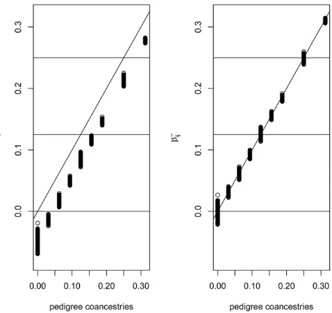
The left-hand plot of Figure 6 compares the coancestry estimates ^bjj9;with the pedigree values for all pairs of
indi-viduals in the pedigree, and reflects the summing to zero by construction of theb^jj9;j6¼j9coancestries, whereas the
ped-igree coancestries are necessarily non-negative. The right-hand plot shows a “correction”of the estimates: we took the set of smallestb^jj9values in the left-hand plot to represent
the unrelated (relative to the assumed-unrelated) founders. If we write^b0as the average value of the set of least-related pairs of individuals then our corrected valuesb^cjj9are
^
bc jj9¼
^
bjj92b^0 12^b0
: (11)
The corrected estimates are clearly close to the pedigree values. However, we are not sure if it is necessary, in general, to undertake this correction process. Whether or not it is applied, theb^values are still relative to those among all pairs of individuals in a study sample. In general, we will not have any individuals identified for which it is justified to assume zero relatedness or zero inbreeding, and we note the com-ment by Thompson (2013)“in most populations IBD within individuals is at least as great as IBD between.”
The distributions of estimates in Figure 7A are tightly clustered around nine values, corresponding to the nine dis-tinct pedigree values i=32;i¼0;1;2. . .6;8;10:A contrast-ing result is shown in Figure 7B, for the standard estimates
(Equation 7), calculated as weighted averages over loci (i.e., taking the ratio of the sums over loci of the single-locus esti-mator numerators and denominators).
There is a current tendency in genome wide association studies (GWAS) to restrict the SNPs used in relatedness estimation to having a minor allele frequency (MAF) above some threshold. For example, theKINGmanual (http://people. virginia.edu/wc9c/KING/manual.html) lists a parameter-minMAF to specify the minimum minor allele frequency to select SNPs for relationship inference in homogeneous popula-tions. The thought is that lesser frequencies give rise to biased values, but that is not likely the case if “ratio of averages” estimates are used. To illustrate the effect of MAF filtering, we applied four different thresholds to our simulated data, and we show the means and SDs for estimates for each of nine pedigree values in Table 7. The estimates are the corrected values – i.e., relative to an assigned value of zero for the least-related class. There is clear evidence for the merits of retaining all SNPs, both in terms of bias and variance: allfi l-tered estimates are downwardly biased, and the stronger the filter, the stronger the downward bias.
We continued a comparison of our proposed coancestry estimates b^ by applying the estimates described by Wang (2014), listed in Table 8, and computed using therelatedR package (Pewet al.2015). Additionally,relatedoffers maxi-mum likelihood estimators, derived by Milligan (2003) and Wang and Santure (2009). They are not computed here, because they require substantial computing time, which may rule them out for genomic data.
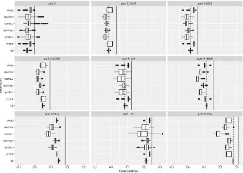
In Figure 8 we display box plots of coancestry estimates for seven alternative estimates, displayed according to nine ped-igree values. The solid line for each panel corresponds to the Figure 5 Pedigree-based coancestry coefficients for simulated data for
135 individuals with 20 founders. Red correspond to low values, yellow to high values of coancestry, white are missing data (unknown inbreeding coefficient of the founders). Black horizontal and vertical lines separate generations in the pedigree. The yellow blocks along the main diagonal correspond to sibships.
pedigree value. The dashed line corresponds to an adjusted pedigree value, where the adjustment is obtained by sub-tracting the mean pedigree coancestry from the pedigree val-ues, and dividing this by 1 – the mean pedigree value to insure that the range of possible values are covered. In Figure 6, we used estimates from the least related individuals to adjust the estimates, whereas here we adjusted the pedigree values to have an overall mean of zero.
All the estimates are negatively biased when compared to the pedigree values. When compared to the adjusted pedigree value, thebestimates show extremely good properties, with no bias, and very small variances. Other estimates, while also closer to these adjusted values, mostly underestimate, but sometimes overestimate (e.g., wang, lynchli) the adjusted pedigree values. The standard estimators (weighted or un-weighted) consistently underestimate the adjusted pedigree values, except for the unrelated class.
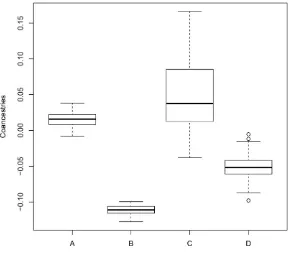
Next, we illustrate how we can recover the average FST from the individual coancestries. For this, we use the pedi-gree described above, but take as founders 10 individuals from each of the two populations (meanFSTbetween these two populations isb^ST¼0:114). Figure 9 illustrates the ac-curacy of ourbestimates (Equation 6) compared with the standard estimates (Equation 7), for the coancestries of pairs of founders (but with the whole pedigree as the reference population). Theb^values for pairs of founders from the same population (Boxplot A in Figure 9) are tightly distributed around 0.016, whileb^’s for pairs of individuals one from each population (boxplot B) are tightly distributed around
20:111: The distribution for the same two categories for the standard estimator (boxplots C and D) is wider, in partic-ular for pairs of individuals originating from the same population.
Theb^ST;i.e., the average^FSTfor the two populations from which the founders originated, is recovered from the individual coancestries as follows: each individual pair coancestry is calcu-lated asb^pjj9¼ ðMe
p jj92Me
p
SÞ=ð12Me p
SÞ(Table 3; the superscriptp highlights that the estimates are taken over all pairs in the pedigree). We are seeking b^STf0¼ ðMe
Sf0
2MeBf0Þ=ð12MeBf0Þ; the overallFSTamong the founders only. The mean coancestry of founders from the same population in Figure 9 (boxplot A) corresponds to ~Sf0¼ ðMe
Sf0
2MepSÞ=ð12Me p
SÞ; and the mean coancestry of founders, one from each population in the same figure (boxplot B) corresponds toBf~0¼ ðMe
Bf0
2MepSÞ=ð12Me p SÞ: Subtracting~Bf0from~Sf0;and dividing byð12Bf~0Þallows elim-ination of MepS and recovery of the expression of ^bSTf0: For our situation, this gives b^STf0¼ ð0:0162ð20:111ÞÞ= ð12ð20:111ÞÞ ¼0:114¼b^ST;as expected.
Discussion
A unified approach
Although there has been general recognition that family and evolutionary relatedness are just two ends of a continuum, we are not aware of previous moment estimates of population structure quantities such asFSTor individual-pair coancestries that rest on this common framework. We have presented estimates that apply equally well to populations and individ-uals. While their statistical properties remain to be fully ex-plored, it is reassuring to see how well they performed in the few simulations presented here.
Although individual-specific inbreeding coefficient, and individual-pair-specific coancestry coefficient moment esti-mates, are used routinely in association studies, we have not seen widespread adoption of population-specificFST mo-ment estimates in evolutionary studies. We have shown here, theoretically and empirically, that these values can differ sub-stantially among populations. This may simply reflect popu-lation size and migration rate differences, but different values for specific loci may also provide signatures of natural selec-tion: see Balding and Nichols (1995), Beaumont and Balding (2004), Foll and Gaggiotti (2008) and Weiret al.(2005) for example. There is a growing literature for Bayesian analyses that address population-specific parameters (e.g., Karhunen Figure 7 Comparison ofb (A) and standard coancestry (B) estimates,
when founders are drawn from a single population.
Table 7 Effects offiltering toLSNPs on coancestry estimate means (and SDs 3100)
Pedigree value
L¼79;069 L¼72;012 L¼56;979 L¼44;061 All SNPs MAF‡0:01 MAF‡0:05 MAF‡0:10
and Ovaskainen 2012; Günther and Coop 2013), although these may not be amenable to analyses of genome-wide var-iant data.
There is also general understanding that identity by de-scent is a relative concept, rather than an absolute concept. This understanding has not led to an apparent recognition that the standard estimates of inbreeding and kinship are not unbiased for expected or pedigree values. Replacing popula-tion allele frequencies by sample values leads to bias in the usual estimates,regardless of sample size. Whenever sample allele frequencies from a study are used to estimate inbreed-ing or coancestry coefficients, the estimators are affected by the inbreeding and coancestry values for all study individu-als. We will come back to this point in the section containing Equation 13
We also stress that all allelic variants, whatever their frequencies, need to be included in the estimation of popula-tion structure and inbreeding or relatedness. The estimates certainly depend on the allele frequencies, and restricting the range of frequencies used may reveal features of interest, but the underlying ibd parameters do not depend on the frequen-cies (see Equation 1 with the ibd interpretation). Exclusion of some alleles based on their frequencies will lead to biased estimates of the parameters as shown in Table 7.
Table 8 Other estimates of relatedness
Method Description
ped The pedigree based relatedness
bij bij;developed here (Equation 4). These values are relative to the mean of the population and hence the mean of these relatedness must be 0
stand.u The standard estimator, Equation 7 average of ratios Identical to the estimator derived by Ritland (1996)
[Equation (4) in Wang (2014)] and also used in GCTA Yanget al.(2011)
stand.w Equation 7, ratio of averages
wang The estimator developed by Wang (2002)
lynchli The estimator derived by Lynch (1988) and improved by Liet al.(1993), Equation (7)in Wang (2014)
lynchrd The estimator derived by Lynch and Ritland (1999) [Equations (5 and 6) in Wang (2014)]
quellergt The estimator derived by Queller and Goodnight (1989) [Equations (2 and 3) in Wang (2014)]
Previous estimates
Weir and Cockerham estimates ofFST:TheFSTestimate of WC84 has been widely adopted, and it performs well for the model stated in that paper: data from a series of independent populations with equivalent histories and sizes. In the pres-ent notation, WC84 assumedui¼u;uii9¼0 for all
popula-tions i and all i96¼i: The estimate was designed to be unbiased for any number of sampled populations, any sample sizes and any number of alleles per locus. The analysis was a weighted one over populations: the average allele frequencies pu for a study had sample size weights,
pu¼Pini~piu=
P
ini for ni alleles sampled from population i. Although ourbestimates do not make explicit mention of allele frequencies, there is implicit use of sample frequencies that are unweighted averages over populations.
Weighting over populations has been discussed by Tukey (1957) and Robertson (1962). Those authors were concerned with bias and variance, and they used the language of variance components, within and between populations. For allele u, these components were given as ð12uÞpuð12puÞ and
upuð12puÞ;respectively, by WC84. Tukey said“In practice, we select two quadratic functions by some scheme involving intuition,find how their average values are expressed linearly in terms of the variance components, and then form two linear combinations of the original quadratics whose average values are the variance components. These linear combinations are then our estimates. Muchflexibility is possible.”The estimates of WC84, Weir and Hill (2002) and Bhatiaet al.(2013) all have this structure, although ratios of linear combinations are taken to remove the allele frequency parameters. Tukey went on to say that the weightswi¼ni(in the present notation)“gives the customary analyses, which treat observations as important and columns [i.e.populations] as unimportant.”Further,“the choice
wi¼1. . .treat the columns as important. This [unweighted] approach is appropriate when the column variance component is large compared with the within variance component.” Robertson (1962) also pointed to sample-size weights for small between-population variance components and equal weights for large values. Bhatiaet al.(2013) were concerned with un-equalFSTvalues so their use of equal weights is consistent with Turkey’s statements. Their work provides simple averages of the different FST values as opposed to averages weighted by sample sizes. For unequalFSTand unequal sample sizes, Weir and Hill (2002) said“the usual moment estimate [with sample-size weights] is of a complex function [of theFST’s].”In our current model of unequal ui and nonzerouii9; we agree that
unweighted analyses (population weights of 1) are appropriate, and that is what we have used in this paper. We note that Tukey’s “flexibility”in the choice of moment estimators, phrased in terms of weights, does not arise with maximum likelihood approaches. If sample allele frequencies are taken to be approximately nor-mally distributed, then REML methods give appropriate and unique estimates.
What are the consequences of using the WC84 estimates when the current model of unequaluiand nonzerouii9is more appropriate? We can show that the expected value of the Weir and Cockerham estimate^uWCis
Eð^uWCÞ ¼uW*2uB*þQ 12uB*þQ :
This expression uses three functions of sample sizes:
n¼Pri¼1ni=r; nci¼ni2n2i=
P
ini and nc¼
P
inci=ðr21Þ: The two weighted averages are uW*¼P
inciu i=P
inciand
uB*¼P i
P
i96¼inini9u ii9=P
i
P
i96¼inini:9 The quantity Q is ½Piðni=n21Þui=½ncðr21Þ:For equal sample sizes,ni¼n; or, for equal values ofFST;uiW¼uW¼uW*¼u;andQ¼0:
Under these circumstances Eðb^WCÞ ¼ ðuW2uBÞ=ð12uBÞ; and we find the WC84 estimator performs well unless ui and/ornivalues are quite different. We stress though that it isðuW2uBÞ=ð12uBÞbeing estimated.
Nei estimates of FST:Although we have phrased estimates in terms of matching proportions, we note that they are the complements of“heterozygosities”M~ ¼12H:~ Our approach usesMeB;the average population-pair allele matching, whereas most previous treatments, from Nei (1973) onwards, use total heterozygositiesH~T¼12Pup2uwherepuis the average sam-ple allele frequency over populations: pu¼
Pr
i¼1~piu=r: For large sample sizes, H~T¼ ðr21ÞH~B=rþH~W=r and Nei’s GST quantity and its expectation, in our notation, are
GST¼12 H~
W
~
HB21
r
~
HB2H~W ;
EðGSTÞ ¼ uW2uB
12uBþr21112uW; (12)
which reduce tob^WTandEð^bWTÞasrbecomes large. Other-wise, the expectation of GST depends on the number r of
populations. This expectation is bounded above by one, con-trary to the claim of Bhatia et al.(2013). Nei and Chesser (1983) and Nei (1987) modified Nei’s earlier approach to remove the effects of the number of populations. Bounds on FST; when that is defined as ð12H~
W
=H~TÞ; were given by Jakobssonet al.(2013).
Jost (2008) pointed out thatGSTdoes not provide a good measure of differentiation among populations, where differen-tiation reflects the collection of allele frequenciespiu;or their sample values~piu:We regarduas an indicator of evolutionary history, rather than of allele frequencies, and we interpret it as probabilities of pairs of alleles being identical by descent. Jost introducedD¼ ðHB2HWÞ=ð12HWÞorD¼ ðuW2uBÞ=uW
as a measure of differentiation among populations. For the two-population drift scenario without mutation,D, unlikebWT;does not have a simple dependence on time, and so does not serve as a measure of evolutionary distance.
Standard coancestry estimates: The expressions in Equa-tion 7 provide unbiased estimates of ujj¼ ð1þFjÞ=2 and
ujj9;j6¼j9when the allele frequencies are known. When study
sample allele frequencies are used, however, the expectations of these expressions, for one locus, are