| INVESTIGATION
Polygenic Adaptation to an Environmental Shift:
Temporal Dynamics of Variation Under Gaussian
Stabilizing Selection and Additive Effects on a
Single Trait
Kevin R. Thornton1 Department of Ecology and Evolutionary Biology, University of California, Irvine, California 92697
ABSTRACT Predictions about the effect of natural selection on patterns of linked neutral variation are largely based on models involving the rapidfixation of unconditionally beneficial mutations. However, when phenotypes adapt to a new optimum trait value, the strength of selection on individual mutations decreases as the population adapts. Here, I use explicit forward simulations of a single trait with additive-effect mutations adapting to an “optimum shift.”Detectable“hitchhiking”patterns are only apparent if (i) the optimum shifts are large with respect to equilibrium variation for the trait, (ii) mutation rates to large-effect mutations are low, and (iii) large-effect mutations rapidly increase in frequency and eventually reachfixation, which typically occurs after the population reaches the new optimum. For the parameters simulated here, partial sweeps do not appreciably affect patterns of linked variation, even when the mutations are strongly selected. The contribution of new mutationsvs.standing variation tofixation depends on the mutation rate affecting trait values. Given thefixation of a strongly selected variant, patterns of hitchhiking are similar on average for the two classes of sweeps because sweeps from standing variation involving large-effect mutations are rare when the optimum shifts. The distribution of effect sizes of new mutations has little effect on the time to reach the new optimum, but reducing the mutational variance increases the magnitude of hitchhiking patterns. In general, populations reach the new optimum prior to the completion of any sweeps, and the times to fixation are longer for this model than for standard models of directional selection. The long fixation times are due to a combination of declining selection pressures during adaptation and the possibility of interference among weakly selected sites for traits with high mutation rates.
KEYWORDSpolygenic adaptation; hitchhiking; linked selection; forward simulation
E
MPIRICAL population genetics seeks to understand the evolutionary histories of natural populations by analyzing genome-wide patterns of polymorphism. The interpretation of observed patterns relies heavily on mathematical models, accompanied by various simulation methods, which make concrete predictions about the effect of evolutionary forces(natural selection, demographic events, etc.) on patterns of variation.
The models of natural selection used to interpret data come primarily from what we may call“standard population genet-ics”models. In these models, mutations have a direct effect on fitness (a“selection coefficient”). Thefitness effects of mutations are most often assumed to be constant over time. For example, background selection is a model of unconditionally deleterious mutations resulting in strong purifying selection (Charlesworth
et al.1993, 1995; Hudson and Kaplan 1995; Cvijovi´cet al.2018). The model of a selective sweep from a new mutation similarly posits that the variant is unconditionally beneficial with a con-stant effect on fitness over time (Maynard-Smith and Haigh 1974; Kaplanet al. 1989; Bravermanet al.1995; Durrett and Schweinsberg 2004), and a similar assumption is made in models of selection from standing genetic variation (Hermisson and Pennings 2005; Berg and Coop 2015).
Copyright © 2019 Thornton
doi:https://doi.org/10.1534/genetics.119.302662
Manuscript received August 26, 2019; accepted for publication October 21, 2019; published Early Online October 25, 2019.
Available freely online through the author-supported open access option.
This is an open-access article distributed under the terms of the Creative Commons Attribution 4.0 International License (http://creativecommons.org/licenses/by/4.0/), which permits unrestricted use, distribution, and reproduction in any medium, provided the original work is properly cited.
Supplemental material available atfigshare:https://figshare.com/articles/simaterial_pdf/ 10046279.
1Address for correspondence: 321 Steinhaus Hall, University of California, Irvine, CA
The effect of natural selection on linked neutral variation has been extensively studied for the case of directional selec-tion on mutaselec-tions with direct effects onfitness (e.g., Kaplan
et al.1989; Stephanet al.1992; Wiehe and Stephan 1993). This framework leads to a natural simulation scheme using the structured coalescent (Kaplan et al. 1988), which has been widely used to study the power of various approaches to detect recent sweeps from new mutations (Fay and Wu 2000; Kim and Nielsen 2004), from standing variation (Innan and Kim 2004; Hermisson and Pennings 2005; Przeworskiet al.2005), from new mutations occurring at a fixed rate in the genome (Bravermanet al.1995; Przeworski 2002), or to test methods to distinguish between various models of adaptation (Garudet al.2015; Schrider and Kern 2016).
The model of Gaussian stabilizing selection around an optimal trait value differs from the standard model in that mutations affect fitness indirectlyvia their effects on trait values. For the additive model of gene action considered here, and considering a single segregating mutation affect-ing the trait, the mode of selection is under- or overdomi-nant in a frequency-dependent manner (Robertson 1956; Kimura 1981). This model has been extended to multiple mutations in linkage equilibrium by several authors (Barton 1986; de Vladar and Barton 2014; Jain and Stephan 2015, 2017b).
The equilibrium conditions of models of Gaussian stabi-lizing selection on traits have been studied extensively (Bürger 2000, chapters 4 and 5). In general, the dynamics are quite complicated, with many possible equilibria exist-ing for the case of many biallelic loci with equal effect sizes and no linkage disequilibrium (Barton 1986). It is also com-mon to assume that the forward and backward mutation rates per locus are equal (Barton 1986; de Vladar and Barton 2014; Jain and Stephan 2015, 2017b). Under these assumptions, and assuming distributions of mutational ef-fects symmetric 0, large-effect variants (e.g., those with effect sizes . 2pffiffiffi2pffiffiffiffiffiVS, where VS is the variance of the Gaussianfitness function) will be near the boundaries while small-effect variants will be at frequencies near one-half (de Vladar and Barton 2014; Jain and Stephan 2017b). Here, large and small effect is with respect to the effect of a variant on the genetic load of a population (de Vladar and Barton 2014).
While thefitness effects of individual mutations on trait values affect theirfixation probabilities, change in the mean phenotype of a population depends on the additive genetic variance (Robertson 1960). When most mutational effects are small and additive,fixations require on the order of the population size in generations because phenotypic change proceeds via thefixation of small-effect mutations, primarily by genetic drift (Robertson 1960). Recent theoretical work has attempted to clarify when sweeps should happen and when adaptation should proceed primarily via subtle allele frequency shifts. Chevin and Hospital (2008) considered the case of a single mutation with a large effect onfitness in a
highly polygenic background evolving according to an infi n-itesimal model. The authors found that sweeps stall at inter-mediate frequencies because frequency shifts in the polygenic background contribute to adaptation. Under models of link-age equilibrium, additive mutational effects, and equal rates of forward and back mutation at a biallelic locus (Barton, 1986; de Vladar and Barton 2014), polygenic traits adapt quickly to a sudden shift in the optimum via directional se-lection (Jain and Stephan 2017b). In an infinitely large pop-ulation, mutations that are rare at the time of the optimum shift mayfix if their effect sizes are not overly large relative to the magnitude of the shift. The number of large-effect sweeps during adaptation depends on the magnitude of the shift and the average effect size of segregating variants (Jain and Stephan 2017b). After the directional phase, selection becomes disruptive, and mutations affectingfitness arefixed or lost to reduce the genetic load of the population.
Under a model of a trait with a small number of phenotypic classes, Höllingeret al.(2019) describe the dynamics of mu-tations following an optimum shift for traits with low muta-tion rates and for highly polygenic traits. The key parameter in their model is Q¼4Nm, where m is the mutation rate relevant to the trait. WhenQ ≲ 1, adaptation primarily oc-curs via complete sweeps. At intermediate valuesðQ10Þ, partial and complete sweeps occur by the time the population has adapted. When Q100, adaptation (defined as when meanfitness has recovered following the optimum shift) pro-ceeds via frequency shifts at many loci.
While the work described above identifies the conditions where sweeps are expected, we do not have a picture of the dynamics of linked selection during adaptation to an opti-mum shift. In large part, the difficulty of analyzing models of continuous phenotypes with partial linkage among sites has been an impediment to a theoretical description of the process. In general, the standard model of a single trait with additive-effect mutations and Gaussian stabilizing selection assumes linkage equilibrium (or quasi-linkage equilibrium) (Turelli 1984; Barton 1986; de Vladar and Barton 2014; Jain and Stephan 2015, 2017b). Höllingeret al.(2019) were able to accommodate partial linkage by simplifying how mutations affect phenotype and focusing on the dynamics up until a particular mean trait value wasfirst reached. In their simplest model, an individual is either mutant or nonmutant, and therefore there are only two phenotypes possible.
signatures. The simulations conducted here are therefore analogous to those used to study the spatial dynamics of linked selection via the structured coalescent (Kaplanet al.
1988; Braverman et al. 1995; Kim and Stephan 2002; Przeworski 2002). The key conceptual difference is that the model of adaptation is changed from constant directional selection to the sudden optimum shift models involving a continuous trait considered in de Vladar and Barton (2014) and Jain and Stephan (2015, 2017b). I also investigate the effect of the recombination rate on the time to adaptation and thefixation time of beneficial mutations with respect to the mean time required to adapt to the new optimum.
Materials and Methods
Modeling stabilizing selection
I modeled a single trait under real stabilizing selection (Johnson and Barton 2005). Mutations affecting trait values arise at ratemper haploid genome per generation according to an infinitely many sites scheme (Kimura 1969). For the majority of results, the effect sizes of new mutations on trait values,g, are drawn from a Gaussian distribution with mean zero and SDsg. Mutations have additive effects on trait value and therefore an individual’s genetic value,z, is the sum of all effect sizes in that individual.
Here, I use the term“locus”to refer to a continuous geno-mic region within which mutation and recombination events occur uniformly. Within a locus, mutations occur at positions according to a uniform continuous distribution according to an infinitely many sites scheme. Thus, each mutation results in a biallelic variant and, in the case of trait-affecting muta-tions, the derived allele affects trait values. What I refer to here as mutations are typically referred to as loci in much of the theoretical literature (Robertson 1956, 1960; Turelli 1984; Barton 1986; de Vladar and Barton 2014; Jain and Stephan 2015, 2017b).
Traits are under Gaussian stabilizing selection, such that fitness,w, isw¼e2ðz2zoÞ
2
2VS , wherezois the optimal trait value
andVSis the sum of the variance infitness plus the environ-mental variance in phenotype (Bürger 2000, p. 160). Figure 1 shows a schematic of the model. For all simulations per-formed here, I useVS¼1.
I modeled an environmental challenge as a sudden opti-mum shift, where the optiopti-mum trait value changed from
zo¼0 tozo.0.
It is important to note that I considered all of the heritable variation for the trait to be modeled in the genomic regions that are explicitly simulated. Thus, the approach is similar in spirit to that of de Vladar and Barton (2014), but with partial linkage. An alternative would be to allow for a genetic back-ground that also evolves, for which we are not tracking mu-tation fates. Chevin and Hospital (2008) used the latter approach to mathematically model the dynamics of large-effect mutations in an infinitesimal background and Stetter
et al.(2018) used a simple version of this method to simulate the dynamics of quantitative traits evolving under truncation selection.
Forward simulation schemes
I ran all simulations using two different Python packages (see
Software availabilitybelow) based on the C++ library fwdpp (Thornton 2014). For a given diploid population size, N, I simulated for 10N generations withzo¼0, at which point the optimum shifted and evolution continued for another 10Ngenerations.
Simulating large genomic regions with only selected variants:To study the dynamics of mutations affecting trait values over time, I evolved populations of size N¼5;000 diploids, where mutations affecting trait values occur uni-formly (at ratem) in a continuous genomic interval in which recombination breakpoints arise according to a uniform Pois-son process with a mean of 0.5 recombination breakpoints per diploid. The mutation rates used were 2:531024, 1023,
and 531023, which is the total mutation rate per haploid
genome. The total mutation rate per diploid, U, was 2m. These mutation rates corresponded to Q¼4Nm values of 5, 20, and 100, respectively, meaning sweeps were expected to be high frequency, mixes of partial and complete sweeps, and adaptation primarily by allele frequency changes, respec-tively, as the population approached the new optimum (Höllingeret al.2019). The three postshift optima used were
zo¼0:1, 0.5, and 1. For all combinations ofmandzo,VS¼1 andsg ¼0:25. At mutation–selection equilibrium, these pa-rameters result in an equilibrium genetic variance given by the“House of Cards”approximation, which is4mfor the definition of mutation rate and theVSused here, and ignoring the contribution of genetic drift (Turelli 1984). With drift, the expectedVGdiffers from the deterministic approximation by a factor of1=½1þVS=ðNs2
gÞ(Bürger (2000), p. 270, Equa-tion 2.8), which is1 for the parameters used here. For the lowmand lowVSused here, the expected genetic variance is therefore small and new mutations are more likely to have large effects relative to standing variation.
For the mutation rates andsg defined above, the muta-tional variances of the trait are 2ms2
g, or 3:2531025, 1:2531024, or 6:2531024, respectively, for each mutation
mutational variance to the environmental variance of
Oð1022Þ, which is the upper limit of the ranges reported
based on experimental results [Lynch (1988) and Falconer and Mackay (1996), p. 349]. Below, I describe simulations varying the distributions of effect sizes, thus changing the mutational variance.
For all combinations ofmandzo, various summaries of the genetic variation (VG;z, etc.) in the population were recorded every generation. In total, I ran 1024 replicates of each pa-rameter combination. For the first 256 replicates, the fre-quency trajectories of all mutations were recorded.
Simulating a 10-locus system with neutral and selected variants:For multilocus simulations, a locus has scaled neu-tral mutation rateu¼4Nmn ¼1000 and scaled
recombina-tion rater¼4Nr¼1000, wheremn is the neutral mutation
rate per gamete at a locus andris the mean number of combination events per diploid at a locus. Mutation and re-combination events occur uniformly along a locus, and each locus is separated by 50 cM. For these simulations, I performed 256 simulation experiments per parameter combination.
Figure 2 shows how a locus is broken up into windows for analysis. Mutations affecting the trait occurred in the sixth out of 11 equal-sized windows in a locus and I analyzed each window separately. Thus, each window hadu¼r90 and mutations affecting trait values were clustered in the middle of each locus (and were intermixed with neutral mutations). In these simulations, the total mutation rate affecting the trait, m, was the sum over loci and the rate per locus was equalðm=10Þ.
At each locus, mutations affecting the trait occurred only in the middle window (Figure 2); therefore, the mean number of recombination events per diploid was0:0045 in the mid-dle window where trait-affecting variants arose. Similarly, the mean number of new mutations per diploid at a given locus affecting the trait was m=5. For the largest mutation rate used hereðm¼0:005Þ, the ratio of recombination events to new mutations affecting the trait in this window was nine to one. The entire genome consisted of 10 such loci, for a total mutation rate ofmand a totalu¼104.
For a model of a single trait under Gaussian stabilizing selection with a constant optimum, the selection coefficient wass¼2Vg2
S[Simonset al.(2018), see also Kimura and Crow (1978)]. Here, VS¼1, and therefore the relevant scaled strength of selection acting on a segregating variant was
Ng2. For many of the results presented here, it is helpful to
treat the dynamics of strongly selected mutations separately. To do so, I define a large-effect variant as havingNg2$ 100,
meaning that the deterministic force of selection is much stronger than that of drift. To vary the probability that a new mutation is of large effect, I performed a second set of simulations, also involving 10 unlinked loci, varying the dis-tribution of effect sizes (DES) such that the probability was thatNg2$100 would take on values of 0.1, 0.5, or 0.75. For
Gaussian DES, the meangis zero, as above, andsgis found by numerical optimization using scipy (Joneset al.2001) to
give the desired PrðNg2$100Þ. I also used gdistributions
with shape parameters equal to either one or one-half, and then found a value for the mean of the distribution using scipy. These shape parameters gave probability density func-tions that were“exponential-like”in shape. For simulations withgDES, I used an equal mixture ofgdistributions with meangand2gsuch that the DES was symmetric around a value of zero. I performed 100 simulation replicates for each parameter combination. Using the argument from above, as-suming hypothetical simulations of a trait with a heritability of one-half, the Gaussian distribution and thegwith a shape of one gave a ratio of the mutational variance to the envi-ronmental variance of 231023 to 331023 when the
pro-portion of new mutations with Ng2$100 was 0.1. These
values were close to the mean of 1023 reported for a
variety of traits [Lynch (1988) and Falconer and Mackay (1996), p. 349].
In a third set of simulations, I variedr¼4Nr, the recom-bination rate within each locus. I ran 256 replicates of these simulations using the tree sequence recording algorithm (Kelleher et al. 2018) implemented in fwdpy11 version 0.3.2. For these simulations, I recorded the entire population as nodes in the tree sequences for each of 200 generations after the optimum shift. Recording nodes from these time points allows them to be analyzed after the simulation has completed. Each replicate was simulated twice. Thefirst run simply output metadata about mutations that reachedfi xa-tion. The second run was performed with the same random number seed as thefirst and used the metadata from thefirst run to track linkage disequilibrium around fixations over time, outputting those data along with the tree sequence for the simulation.
Genome scan statistics from multilocus simulations
The 10-locus simulations described above were used to look at the temporal dynamics of several population–genetic sum-maries of a sample. Each of the 10 loci consisted of 11 non-overlapping windows (Figure 2) and all summary statistics were calculated on a per-window basis. I used pylibseq ver-sion 0.2.1 (https://github.com/molpopgen/pylibseq), which is a Python interface to libsequence (Thornton 2003), to cal-culate all genome-scan statistics. All statistics were obtained from 50 randomly chosen diploids.
z-scores for the nSL statistic: Individual values of thenSL
statistic (Ferrer-Admetllaet al.2014) from thefirst and last window of each locus were binned into intervals of size 0.1 based on derived frequency. These windows were used be-cause they were the furthest from mutations affecting trait values, and thus the least affected by linked selection. The data from all loci were combined, and the means and SDs of each bin were used to obtainz-scores for markers from the remaining windows.
models and discoal (Kern and Schrider 2016) version 0.1.1 for all simulations of selective sweeps. All simulation outputs were processed using pylibseq version 0.2.1.
Software availability: I used fwdpy version 0.0.4 (http://
molpopgen.github.io/fwdpy) compiled against fwdpp
ver-sion 0.5.4 (http://molpopgen.github.io/fwdpp) for single-region simulations. I used fwdpy11 versions 0.1.4, 0.2.1, 0.3.2, and 0.5.1 (http://molpopgen.github.io/fwdpy11) for all multiregion simulations. fwdpy11 is also based on fwdpp, and includes that library’s source code for ease of installation. Both packages were developed for the current work, but only the latter will be maintained.
I used the Python package pylibseq version 0.2.1 (http://
pypi.python.org/pypi/pylibseq/0.2.1), which is a Python
in-terface to libsequence (Thornton 2003), to calculate popula-tion–genetic summary statistics.
All of these packages are available under the terms of the GNU Public License fromhttp://www.github.com/molpopgen. The specific software versions used here are available for Linux via Bioconda (Grüninget al.2017), with the exception of fwdpy11 0.2.1, which must be installed from source. I have made all Python and R (R Core Team 2016) scripts for this work available
athttp://github.com/molpopgen/qtrait_paper.
Open source tools used:Data processing and plotting relied heavily on the following open-source libraries for the R lan-guage (R Core Team 2016): dplyr (Wickham and Grolemund 2017), ggplot2 (Wickham and Grolemund 2017), land attice (Sarkar 2008), as well as the following Python libraries: pan-das (McKinney 2017), numpy (VanderPlas 2016), matplotlib (Hunter 2007; VanderPlas 2016), and seaborn (http://
seaborn.pydata.org). The sqlite3 library (www.sqlite.org)
facilitated data exchange between Python and R via the pandas and dplyr libraries, respectively.
Data availability
The authors state that all data necessary for confirming the conclusions presented in the article are represented fully within the article. Supplemental material available atfigshare:
https://figshare.com/articles/simaterial_pdf/10046279.
Results
Single-region results
In this section, I describe simulations of a large contiguous region with mutations affecting the trait occurring uniformly throughout the region. The technical details of the simulation parameters are given in theMaterials and Methods. Briefly, I evolved populations for 10Ngenerations to mutation–selection equilibrium around an optimum trait value of zo¼0, at which pointzowas changed to 0.1, 0.5, or 1.0 and evolution continued for another 10N generations. These simulations may be viewed as similar to the numerical calculations in de Vladar and Barton (2014) and Jain and Stephan (2017b), but with loose linkage between selected variants, whereas the previous studies assumed linkage equilibrium and I allowed for new mutation after the optimum shift. They differ from the approach of Höllinger et al.(2019) in that I simulated continuous traits and did not stop evolution once a specific meanfitness wasfirst reached.
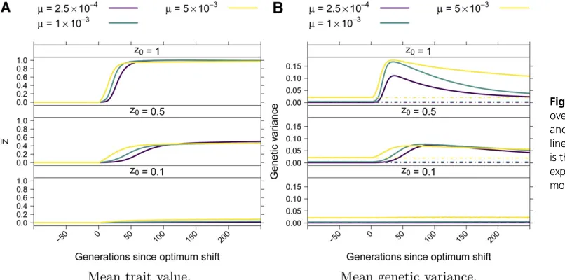
The mean trait value,z, rapidly approached the new op-timum, typically reaching the new optimum within 100 gen-erations [Figure 3A, see also de Vladar and Barton (2014), Jain and Stephan (2017b), and Höllingeret al.(2019)]. Prior to the optimum shift, the average genetic variance was given by 4mVS[Turelli (1984) and Figure 3B]. Following the opti-mum shift, the genetic variance spiked as the population adapted [see also de Vladar and Barton (2014) and Jain and Stephan (2017b)], and then recovered to a value near 4mVSwithin200 generations when the mutation rate was small and took longer to return to equilibrium when the mu-tation rate was higher.
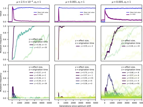
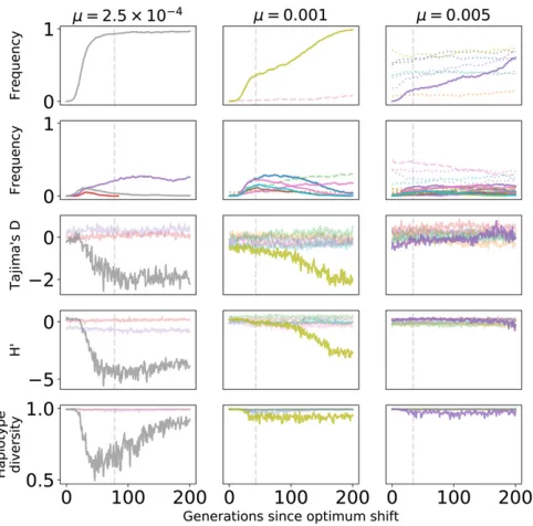
Figure 4 shows examples of the dynamics ofz,VG, and of mutation frequencies following the optimum shift. Each ex-ample is a single simulation replicate. The top row of plots
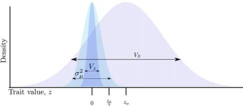
Figure 1 Schematic of the model. A Wright–Fisher population evolves to equilibrium around an optimum trait under Gaussian stabilizing selection with mean zero, where the parameterVSrepresents the intensity of selec-tion against extreme trait valuesðw¼e2z2=2VSÞ. At equilibrium, the mean
trait value is z0 and the genetic variance VG equals the phenotypic varianceVz. Mutations arise at a constant rate with effect sizes,g, drawn from a Gaussian distribution with mean zero and variances2
g. The optimum
then shifts to zo.0, such thatw¼e2ðz2zoÞ2=2VS. During adaptation,z
approaches zo due to allele frequency change and new mutations. At any point during adaptation, mutations with effect sizesg.ðzo2zÞ=2 will overshoot the optimum if they reach high frequency orfix.
shows thatzquickly reachedzofor the individual replicates. The approach ofztozocorresponded with a substantial in-crease in the genetic variance, similar to what is shown for the average genetic variance over time in Figure 3B. The middle row of panels in Figure 4 shows the frequency dynam-ics of mutations that eventuallyfixed. Importantly,ztypically reachedzobefore thefirstfixation had occurred (see Supple-mental Material, Figure S1 for details over a shorter time-scale). The legends the panels in Figure 4 contain the effect sizes of variants whereNg2$100. The legends also contain
the origin times,o, of these large-effect mutations, measured as generations since the optimum shift.
For these examples, mutations with large effects on trait valuefixfirst, as predicted by Robertson (1956). In Figure 4, fixations of large effect typically have origin times close to zero, meaning that the mutations arose close to the time of the optimum shift. This observation is expected as such mutations contribute significantly to genetic load, and thus their equilib-rium frequencies prior to the optimum shift should be near the boundaries (de Vladar and Barton 2014; Jain and Stephan 2015, 2017b). Here, because of the one-way mutation model, such large-effect variants are at frequencies near zero.
Thefinal row of plots in Figure 4 shows the dynamics of mutations that reached a frequency of$1% but were even-tually lost from the population. Large-effect mutations only exist for a relatively brief period of time after the optimum shift, after which most segregating variation reaching appre-ciable derived allele frequencies are of relatively small effect. An important observation in thefinal row of Figure 4 is that, for a short time following the optimum shift, several inter-mediate-frequency mutations with large effects on trait val-ues may be segregating. Many of these variants are adaptive ðg.0Þbut will only make short-term contributions to adap-tation prior to their loss. The dynamics of these muadap-tations recapitulate results from de Vladar and Barton (2014): due to epistatic effects onfitness, some mutations that are initially
beneficial later become deleterious and are removed. Figure S1 shows the data from Figure 4 over a shorter timescale, allowing a more detailed look at the dynamics of mutations during adaptation.
Figure 4 suggests thatfixation times are rather long, in the order of Ngenerations even for mutations with largeNg2.
These longfixation times are in fact typical, and large-effect mutations typicallyfix inN=2 toNgenerations (Figure S2), which is long relative to the deterministic expectation for strongly selected sweeps from new mutations (Stephan
et al.1992). Large-effect mutations that reachfixation arise close to the time of the optimum shift (Figure S3) and typi-cally show shorterfixation times (Figure S4). In general, the numbers of sweeps from new mutations and from standing variants are similar, although fixations of smaller-effect standing variants are more common in simulations with higher m (Figure S5). In Figure S5, a sweep from a new mutation is defined as a mutation arising within 100 genera-tions of the optimum shift and then reachingfixation. While somewhat arbitrary, this definition is justified by the rapid mean time to adaptation (Figure 3). In this model, large-effect standing variants that fixed after the optimum shift were rare at the time of the shift (Figure S6). Small-effect mutations were also typically rare at mutation–selection bal-ance, in particular when the mutation rate was small (Figure S6).
For the parameters simulated here, and for the genetic map simulated here (Figure 2), Figures S3, S4, and S6 suggest that large-effect fixations occur from both new mutations and from standing variation, with more large-effectfixations oc-curring whenmis smaller and/or the optimum shift is larger. Thus, we may predict that large-effect fixations from new mutations may show signs of“hard sweeps,”such as an ex-cess of high-frequency-derived neutral variants (Fay and Wu 2000; Zenget al.2006). Given that large-effectfixations from standing variation are typically rare at the onset of directional
selection (Figure S6), we may also expect them to affect linked neutral variation (Przeworski et al. 2005; Berg and Coop 2015). For the parameters simulated here, fixations from variants that are common at the time of the optimum shift have small effects on trait values (Figure S6). Thefi xa-tion of such mutaxa-tions are unlikely to generate the patterns of haplotype diversity associated with “soft sweeps” because such patterns require strong selection on mutations at inter-mediate frequencies (Garudet al.2015).
Fitness effects of mutations during adaptation
In this section, I explore in more detail the strength of selection on individual mutations during the directional phase of se-lection. These dynamics are relevant to the longfixation times noted in the previous section and also to the extent to which hitchhiking will affect patterns of linked variation, which is the
topic of the next section. As the focus of the remaining sections will be on patterns of variation during adaptation, we switch from simulating a single large region to simulating 10 unlinked regions. The only difference between these simulations and those described above is the genetic map, and the position of mutations affecting trait values (see theMaterials and Meth-odsfor technical details).
Figure 5 plots the dynamics of mutations in a 10-locus system for one replicate of each of the three mutation rates used here. In each column, the gray vertical line is the time the populationfirst reaches a mean trait value of 0:9zo, which corresponds to a meanfitness of$0.9 for each replicate. For simplicity, we will call this the time of adaptation. The top row of Figure 5A shows the frequency trajectories of muta-tions that eventuallyfixed. These replicates were chosen be-cause each had onefixation of a strongly selected mutation
with a similar effect size. As the mutation rate increases, the genetic background of these fixing variants becomes more polygenic. As a result, the initial rate of frequency change of thefixation lessens because other mutations are involved in the response to the optimum shift, some of which may contribute to adaptation but notfix in the long-term. For all replicates, the fixations are at different loci (separated by $ 50 cM) with one exception. For the high-mutation rate case, the locus with the large-effect fixation alsofixed one mutation with smallg.
Figure 5B shows the frequency dynamics of mutations arising prior to adaptation that were eventually lost. As the mutation rate increases, there are more large-effect mu-tations increasing in frequency during adaptation. For the lowest mutation rate simulated here, two such muta-tions are decreasing in frequency prior to adaptation. At m¼0:001, four strongly selected mutations sweep to fre-quencies .0:10 and are later lost. Form¼0:005, several large-effect mutations experience more modest increases in frequency during adaptation. From left to right, the columns of Figure 5, A and B show that allele frequency changes are less dramatic prior to adaptation as the mutation rate in-creases. These results are consistent with the theoretical predictions from Höllingeret al.(2019) that the dynamics
of mutations on the timescale of adaptation are dependent on 2NU.
The second row in Figure 5 shows the mean deviation of a genotype with a given mutation standardized by the SD in trait values (thez-score). The mutations thatfix (Figure 5A) are all initially found in heterozygous genotypes with trait values multiple SDs greater than the mean. Such mutations are not necessarily the largest-effect variants present at the time of the optimum shift, which is seen for the two higher mutation rates in Figure 5. The mutations that did eventually fix were initially at higher frequencies and/or associated with higher-fitness genotypes than large-effect mutations that were eventually lost.
As the population adapts, the deviation in trait value (from the population mean) for a mutation with a given effect size decreases. These z-scores decrease because the genetic variance transiently increases following the optimum shift (Figure 3B) (de Vladar and Barton (2014); Jain and Stephan (2017b) because mutations are increasing in fre-quency and the variance is a function of allele frefre-quency times the squared effect size. Mutations causing larger de-viations are expected to become lost, as seen most clearly in thefirst column of Figure 5B: the blue and green muta-tions over- and undershoot the optimum, respectively. At
Figure 5 Phenotypic andfitness effects offixations and losses. The data shown are for a single simulation replicate withsg¼0:25,zo¼1, and the mutation ratemshown at the top of each column. The mutation rate shown is the sum over loci and individual loci mutate at equal ratesðm=10Þ. In all panels, solid lines refer toNg2$100, dashed lines 10#Ng2,100, and dotted lines 1#Ng2,10. The vertical line is the generation when the mean trait valuefirst crossed 90% of the new optimal valueð0:9zoÞ. (A) The dynamics offixations. The top row shows the frequency trajectory of mutations that eventually reachedfixations. For mutations withNg2$10, the legend showsNg2, and the mutation’s origin andfixation times in parentheses, scaled so that zero is the time of the optimum shift. Defining ana2genotype to be any genotype containing at least one copy of these“focal” mutations, the second row shows the mean deviation from the mean trait value for the focal genotypes, standardized by the phenotypic SD. Thefinal row shows the mean relative deviation infitness fora2genotypes. The horizontal line in the last row is placed at the reciprocal of the population size
low mutation rates, there is a tendency to slightly over-shoot on average (Figure 3) because such mutations will have larger initial increases in allele frequency than smaller-effect variants.
Finally, we can turn to the longfixation times. These are, in part, due to the decreasing strength of selection on individual mutations during the time period where directional selection occurs. Thefinal row of Figure 5 shows the relative deviation due to genotypes carrying each mutation over time. As expected, genotypes with fitness above the mean increase in frequency, and these genotypes are associated with trait values multiple SDs closer to the new optimum. As the mean trait value approaches the new optimum, the relative excess fitness of these genotypes declines, approaching the recipro-cal of the population size. Once the population has adapted, these mutations have small effects on phenotypic variation and their long-term dynamics are governed by underdomi-nant selection against phenotypic variance (Robertson 1956; Kimura 1981). The underdominant selection means that mu-tations with frequencies greater than one-half will be weakly favored and are expected tofix, and those with frequency less than one-half will most likely be removed from the popula-tion. The smallfitness differences among genotypes at the time of adaptation predict that fixation times will be slow due to relatively weak selection (Figure 5). Note that all of the sweeping alleles in Figure 5 are from standing variation
(origin times ,0) and are rare at the onset of directional selection (also see Figure S6).
Finally, traits with higher mutation rates have larger num-bers of small-effect mutations segregating prior to adaptation (Figure 5). Once the population is adapted, the deviations from meanfitness tend to be small for most genotypes and the large-effect mutants are not yet fixed, implying that in-terference (Hill and Robertson 1966) may also increasefi xa-tion times when the mutaxa-tion rate is higher. We will return to the role of interference below. The observation in Figure 4 and Figure 5 of mutations not reachingfixation by the time the new optimum is hit is consistent with previous results from other authors (Chevin and Hospital 2008; Jain and Stephan 2017b; Höllingeret al.2019).
Dynamics of linked selection in a multilocus system
I now describe the temporal dynamics of genetic variation over time in a 10-locus system. The technical details of the simu-lations are identical to the previous section, and are described in detail in theMaterials and Methods.
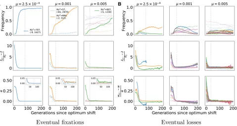
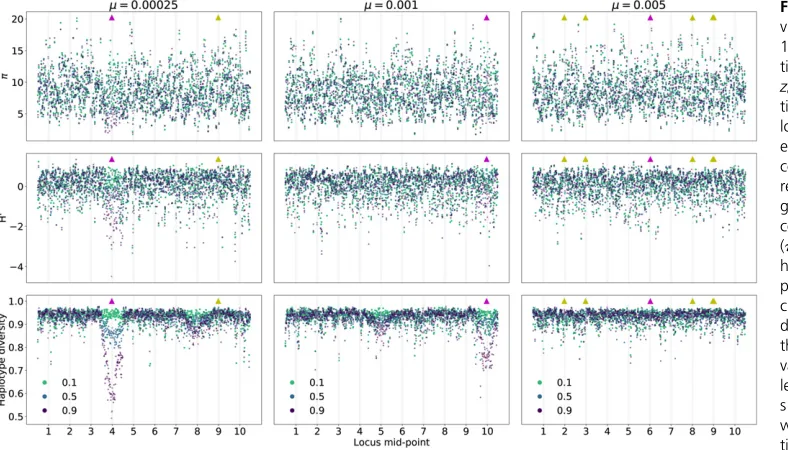
Figure 6 summarizes patterns of variation in the central window (Figure 2) of each locus where large-effect muta-tions segregate during adaptation to the new optimum. The figure is based on the data from Figure 5. Thefirst two rows plot the frequency trajectories of eventualfixations and los-ses, and the next three rows summarize patterns of variation calculated from a random sample of individuals. These sum-maries of variation only show deviations from equilibrium values consistent with positive selection at loci where large-effectfixations occur. Further, the deviations are more pro-nounced when the mutation rate is smaller. The partial sweeps occurring at intermediate mutation rates (middle col-umn of Figure 6) are not associated with strong signals of hitchhiking, at least when the sample size is relatively small, as is the case here. The time when a given statistic shows its maximum departure from equilibrium values differs for each statistic and, for the replicate withm¼0:001, the maximum departure may occur 100 generations after the time to adaptation. However, visually one could argue that haplotype diversity tends to minimize closer to the time to adaptation than the summaries of the site frequency spectrum.
Figure 7 shows patterns of variation along each of the 10 loci from an additional simulated replicate for each of the parameters shown in Figure 5 and Figure 6. Each line corresponds to a different time point in the approach to the new optimum value ofzo¼1, showing data for thefirst time the population mean trait value crosses the thresholds of
z$0:1, $0:5, and $0:9. While the values are noisy along
a genome, it is apparent that directional selection is affecting patterns of variation at linked sites in the replicates with smaller mutation rates. In the leftmost column, where m¼2:531024, an excess of high-frequency-derived variants
is seen at locus 4, along with a reduction in haplotype di-versity. A standing variant of large effect swept to high fre-quency at this locus during adaptation. In the middle column ðm¼1023Þ, one sees a less-dramatic reduction in haplotype Figure 6 Signals of directional selection in single replicates of a 10-locus
system. The data shown are based on the same simulations as in Figure 5. Thefirst two rows show frequency trajectories forfixations and losses, with the colors indicating the locus where the mutation is found. The vertical gray line is the generation when the mean trait valuefirst crosses 90% of the optimal trait value. The remaining rows show Tajima’sD
Tajima (1989),H9(Zenget al.2006), and haplotype diversity in a random sample of 50 diploids, calculated using genotypes taken from the central
diversity at locus 10, where a strongly selected standing var-iant reached high frequency. For these two replicates, there is some evidence of reduced haplotype diversity at loci 8 and 5, respectively, that is not associated with anyfixations. In the final column, wherem¼531023, there are no obvious
tem-poral nor spatial patterns to variation in diversity levels, and the largest deviations from the background are not associated with thefixation of beneficial mutations.
Overall, Figure 6 and Figure 7 suggest that patterns of strong hitchhiking are more likely at loci where large-effect mutationsfix. Moreover, such mutations must arise on aver-age before the mean time to adaptation. Below, when looking at average patterns of variation over time and along ge-nomes, we will distinguish patterns of variation wherefi xa-tions meeting these condixa-tions occur from the mean pattern expected from a randomly chosen locus.
The site-frequency spectrum over time
The expected histogram of mutation frequencies in a sample (the site-frequency spectrum) is a geometrically decreasing function of increasing mutation frequency under the standard neutral model (Wakeley 2008). Departures from this tion are often summarized as single numbers whose expecta-tions are0 under this null model. In this section, I describe the average dynamics of two widely used statistics (Tajima 1989; Zenget al.2006) as a function of both time since the optimum shift and of distance from trait-affecting mutations.
Figure 8 shows the average behavior of Tajima’sD(Tajima 1989) over time. Figure 8A shows the meanDper window, averaging across loci and across replicates. Prior to the opti-mum shift, the mean D is negative in the central window containing selected variants. For highly polygenic traits, the
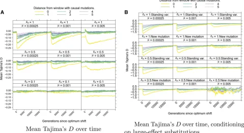
equilibriumDis 20:1 in this window due to a large num-ber of rare deleterious alleles segregating. After the optimum shift, D becomes more negative when the optimum shift is large and the mutation rate is smaller. In linked windows, the magnitude of the change in averagedDdecays rapidly with increasing genetic distance.
Averaging over loci experiencing large-effect fixations, Figure 8B shows a stronger hitchhiking pattern centered on the window containing selected variants. Although the de-viation inDfrom equilibrium decays relatively quickly both along a chromosome and over time, large-effect substitutions generate sufficiently negativeDvalues that such loci will be enriched in the tails of empirical distributions of the statistic. Qualitatively similar patterns hold for the overall reduction in diversity (Figure S7) and the H9statistic (Figure S8). The latter statistic returns to equilibrium rather rapidly, consistent with previous results (Przeworski 2002).
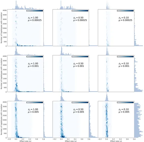
Here, large-effectfixations from new mutations and from standing variants have similar average effects on statistics likeD
andH9(Figure 8 and Figure S8). Figure 9 shows the number of haplotypes at a locus associated with sweeps from standing variation as a function of the effect size of the variant. Here, a haplotype is defined as a unique genotype at a locus, including all neutral and nonneutral variants. Large-effect sweeps from standing variation are either extremely rare (at highm) or are rare at the time of the optimum shift whenmis small, and are usually associated with few (and often only one) haplotypes at the onset of directional selection (Figure 9).
Power to reject the null model using the site-frequency spectrum
Figure S9A shows the power to detect a value of D more negative than expected under the standard neutral model,
Figure 7 Patterns of genetic variation along genomes in a 10-locus system during adapta-tion to an optimum value of
zo¼1 andsg¼0:25. The
after applying a multiple testing correction such that the per-window rejection rate under the null model is 0.05. The overall power of the test is low due to the number of tests performed (one per window) and is consistent with pre-vious work (Bravermanet al.1995; Przeworski 2002). How-ever, the set of loci representing“significant”deviations from the null model are enriched for large-effect substitutions (Figure S9B), of which there are relatively few per replicate (Figure S10). When mutation rates are smaller, significantD
values are most common at loci where large-effect mutations fix. As the trait becomes more polygenic and/or the optimum shift is less drastic, the enrichment shifts toward sweeps from standing variation.
The behavior ofH9is similar to that ofD, but power de-creases more rapidly with time since the optimum shift [Fig-ure S11A; also see Przeworski (2002)]. The behavior of a related test, the composite likelihood ratio test of Nielsen
et al.(2005), evaluated using SweeD (Pavlidiset al.2013), is qualitatively similar to that ofH9(Figure S12).
Haplotype homozygosity
Rapid increases in allele frequency due to selection will result in long stretches of homozygosityflanking the selected mu-tation (Kim and Nielsen 2004). Summaries of haplotype ho-mozygosity are widely used to detect recent selection (Voight
et al. 2006; Ferrer-Admetlla et al. 2014) and are indirect
summaries of the underlying linkage disequilibrium in the data (Sabatti and Risch 2002).
The nSL statistic (Ferrer-Admetllaet al.2014) measures the ratio of homozygosity on the ancestral allele to that on the derived allele for each variant in the data. A negative value of the statistic implies longer runs of homozygosity around the derived allele. Figure S13 shows the average behavior of
z-scores obtained from binningnSLscores by derived allele fre-quencies (see theMaterials and METHODS). The signal of strong positive selection, indicated by a negativez-score, is short-lived, and only observed when the mutation rate is smaller and the optimum shift is large. The signal is also restricted to regions closest to where selected mutations arise.
Shortly after the optimum shift, the meanz-score becomes positive (Figure S13). This temporal dynamic is qualitatively similar to what is seen under standard models of selective sweeps, as the time since the sweep moves further into the past (Figure S14). Thus, the positivez-scores in Figure S13 may be interpreted as either older sweeps from new mutations or strong sweeps from common variants. However, the latter class of sweeps does not occur in these simulations (Figure 9). This difficulty in interpretation is a general issue arising from the fact that patterns of variation due to strong sweeps from standing variation overlap considerably with those of older sweeps from new mutations (Schrideret al.2015).
A related class of statistics designed to detect strong sweeps from standing variation are based on the overall haplotype
diversity in a window (Garud et al. 2015). The temporal patterns associated with these statistics are again short-lived and are all in the direction of reduced overall haplotype het-erozygosity, which is a signal of strong sweeps from new mutations (Figures S15, S16, and S17).
Robustness to variation in the recombination rate
In this section, I explore the effect of varying the scaled recombination rate within a locus, r. At higher mutation rates, longer fixation times are more likely as r decreases
(Figure 10). In individual replicates, there is a tendency to-ward negative disequilibrium among beneficial mutations (g.0, Figure S18), suggesting a role for interference among selected sites affecting times tofixation (Hill and Robertson 1966; Felsenstein 1974). In the previous sections, the ratio of r to u within loci was one, which is roughly “human”-like (Dumont and Payseur 2008; Ségurelet al.2014). For species like Drosophila melanogaster, where ru (Haddrill et al.
2005),fixation times will be much shorter on average (Figure 10). Note that the effect of recombination rate on fixation
Figure 9 The number of haplotypes associated withfixations from standing variation of different effect sizes. Each panel shows the effect size of a
time is most dramatic form¼0:005, which is also the part of the parameter space explored here wherefixations of larger-effectðNg2$1000Þare rare.
The within-locus recombination rate has no discernible average effect onznor onVG(Figure S19). The differences in the height of the“spike”inVGwhenm¼2:531024show no
clear pattern withrand are thus attributable to Monte Carlo error in estimating a second-order statistic from 256 replicates. Unlike the mean trait value and variance, the mean tem-poral dynamics of summaries of variation data are strongly affected byr(Figure S20) as expected (Kaplanet al.1989; Bravermanet al. 1995). Figure S21 shows how the within-locus recombination rate affects patterns of haplotype diver-sity in a 10-locus system withsg¼0:25. Whenris small, the impact of linked selection is much more apparent. These ef-fects of the local recombination rate on patterns of hitch-hiking are expected from standard theory of directional selection, because both the magnitude and extent along the genome of linked selection depend on the ratio of the recom-bination rate to the selection coefficient (Kaplanet al.1989; Durrett and Schweinsberg 2004; Nielsenet al.2005).
Varying the DES
The results described in the previous sections are based on a Gaussian DES whose SD is held constant. In this section, I vary the DES such that the fraction of mutations withNg2$ 100
varies, and compare the average dynamics of adaptation and
patterns of hitchhiking. I also compare a Gaussian distribu-tion to agdistribution with different shape parameters. To simplify the presentation, I only show results for the case of a large optimum shiftðzo¼1Þ, which is the case resulting in
the most extreme hitchhiking signals. I compare the results of Gaussian distributions of effect sizes to twog distributions with shape parameters of one and one-half.
Varying the fraction of large-effect mutations has a weak effect on the mean time to reach the new optimum, with traits with low mutation rates adapting more slowly on average when the majority of variants are of small effect (Figure S22A). This observation should be unsurprising as the population must wait longer for a strongly selected mutation in this case.
Patterns of variation expected due to hitchhiking are more extreme whenPrðNg2$100Þis small, as the population has
to wait longer for strongly selected variants (Figure S23). The overall pattern is that the average differences between DES are subtle, withgdistributions showing less-extreme hitch-hiking patterns (negative values) on average than the Gauss-ian DES. However, this difference between DES is only observed when both the mutation rate and the proportion of new mutations of large effect are both small.
Discussion
I have used simulations to describe the average behavior of selected and neutral mutations during the adaptation of a
quantitative trait to a single, sudden shift in the optimal trait value. The genotype-to-phenotype model considered here is the classic model of evolutionary quantitative genetics, as-suming strictly additive mutational effects on trait values with fitness determined by Gaussian stabilizing selection (Turelli, 1984; Barton 1986; Bürger 2000). The primary goal here was to merge this model of a phenotype with the simulation methods commonly used in population genetics to study the effect of natural selection on the dynamics of linked neu-tral variation (Kaplan et al. 1988, 1989; Braverman et al.
1995; Przeworski 2002; Innan and Kim 2004).
The simulations performed here have several important differences from recent theoretical treatments of adaptation to sudden optimum shifts (see below). However, the condi-tions for a selective sweep are consistent with predic-tions made using theoretical results from Jain and Stephan (2017b) and Höllingeret al.(2019). Direct comparison with the quantitative predictions from Jain and Stephan (2017b) is difficult because their expressions depend on the assump-tion of equal forward and backward mutaassump-tion rates at each position. However, several qualitative comparisons can be made. First, the simulations presented here are comparable to the “most effects are large”case from Jain and Stephan (2017b) because the trait varianceincreasesduring adapta-tion [also see de Vladar and Barton (2014)] due to large-effect mutations moving from low to intermediate frequency. Mutations with large effects on trait values at the time of the optimum shift are most likely to rise in frequency (Figure 4 and Figure 5), although mutations that eventuallyfix are not necessarily those with the largest effect size. When several large-effect mutations cosegregate, those with the highest initial frequencies tend to reachfixation. If initial frequencies are similar, the variant with the highest initialfitness typically fixes. For a given DES, faster sweeps are more likely at lower mutation rates.
Regimes where the genetic variance decreases during adaptation are not possible for any of the simulations pre-sented here. The decrease in variance is seen in the “most effects are small”domain where the equilibrium frequency of variants prior to the optimum shift is one-half, which maxi-mizes the variance (de Vladar and Barton 2014; Jain and Stephan 2017b). Adaptation to the new optimum displaces allele frequencies, reducing the variance from its maximum value [see, for example, figure 9 of de Vladar and Barton (2014)]. However, the equilibrium frequency of one-half for small-effect mutations requires equal rates of forward and back mutation (de Vladar and Barton 2014; Jain and Stephan 2017b, and is therefore incompatible with the in-finitely many sites assumption made here.
When considering the pattern of hitchhiking at a locus, the presence or absence of a large-effectfixation at a locus is a reliable predictor of the magnitude of hitchhiking patterns. As expected, suchfixations are more common when the mutation rate is smaller (Höllingeret al.2019) and thus strong depar-tures from equilibrium patterns of variation are not expected for more polygenic traits (Figure 8). For the optimum shift
model considered here, the strength of selection is not con-stant over time [Figure 5; see also Kimura (1981)]. Thus, genotypes containing variants that were initially strongly fa-vored by selection are subject to much weaker selection by the time the population has reached the new optimum. This weakening of selection increasesfixation times to the order of the population size (Figure S2), which is much longer than the timesNgenerations expected for directional selection in large populations (Stephanet al.1992).
The exploration of hitchhiking signals here involved the simulation of 10 unlinked loci within which mutations affect-ing the trait were concentrated in a central window (Figure 2). While the ratio of recombination to mutation events is at least nine to one for the majority of the results shown here (see
Materials and Methods), it is possible that signals of selection are made more pronounced by the localization of selected mutations and should be explored further.
Here, the number of selected mutations segregating over time ranged from dozens to several hundred, as a function of the underlying mutation rate (Figure S24). At high mutation rates, the number of segregating loci are roughly the same as some of the results presented in de Vladar and Barton (2014). However, the partial linkage among sites in this work leads to some negative linkage disequilibrium (Figure S18), which is a signal of interference (Hill and Robertson 1966; Felsenstein 1974). This interference has little effect on the mean time to adaptation, butfixation times are increased. The lack of effect on time to adaptation is driven by initial largefitness differ-ences among genotypes [Figure 5, also see Höllingeret al.
(2019)]. Once the population is close to the new optimum, selection on individual genotypes is much weaker (Figure 5), setting up the conditions for interference to affect fixation times (Hill and Robertson 1966).
The DES has different effects on properties of the trait than on patterns of hitchhiking. The mutation rates used here span the parameter space from partial and complete sweeps being most common to the optimum being reached via allele fre-quency shifts of many mutations (Figure 4; Höllinger et al.
2019). In general, the mean time to adapt is not strongly affected by the DES if the fraction of new mutations of large effect is constant (Figure S22A). For a given mutation rate, lowering the mutational variance lowers the probability of a strongly selected mutation, increasing the waiting time until such mutations arise, and thus resulting in stronger signals of hitchhiking Figure S23). When the trait is more polygenic, the average patterns of variation are not strongly dependent on the DES nor on the proportion of new variants with large effect (Figure S23).
selectionðVSÞpreserves the rank orders offitness for all ge-notypes, merely changing how fit they are in an absolute sense. One could randomly reassign effect sizes at the time of the optimum shift in an attempt to approximate a gene-by-environment interaction. However, such a procedure would be arbitrary, and thus not represent a principled model for generatingdetectablesoft sweep patterns. Rather, it is tempt-ing to invoke a need for pleiotropic effects to have large-effect mutations segregating at intermediate frequencies at the time of the optimum shift, with the shift itself accompanied by a change in the covariance between trait values and fitness.
It is important to note a key methodological difference between this work and that of other authors. Höllingeret al.
(2019) stopped their simulations when the population was close to the new optimum while the simulations conducted here allowed evolution to continue much longer. Thus, on the timescale during which the population adapts,fixations are not observed whenQis high [seefigure 4 of Höllingeret al.
(2019)]. Here, we observe fixations of large effect for the mutation rates corresponding to Q¼4Nm¼100 (Figure 4), which Höllingeret al.(2019) show is the parameter range where adaptation occurs primarily by changes in allele fre-quency. These results are consistent with the theoretical pre-dictions from Höllingeret al.(2019), as thefixations in the simulations described here take place on timescales longer than the mean time to reach the new optimum. In the right-most column of Figure 4, the population has adapted quickly, with the fixations occurring over a much longer timescale (Figure S1). Likewise, the leftmost column of Figure 4 corre-sponds toQ¼5, where we observe a mixture of partial and complete selective sweeps by the time the new optimum is reached, which is expected from the theory presented in Höllingeret al.(2019).
This work [and that of Höllingeret al.(2019)] differs from the analytical and numerical work of de Vladar and Barton (2014) and Jain and Stephan (2015, 2017b) in several key aspects. First, we consider irreversible mutation here [the infinitely many sites model of Kimura (1969)], while de Vladar and Barton (2014) assumed equal rates of forward and reverse mutation [see also Barton (1986) and Jain and Stephan (2015, 2017b)]. The infinitely many sites model used here was chosen because it is the most commonly used mutational model for investigating the effects of linked selection during adaptation (e.g., Bravermanet al.1995; Przeworski 2002; Przeworskiet al.2005). I also allowed for partial linkage among sites, which is a key difference from the work based on the Barton (1986) framework, which assumes free recombination. As noted above, partial linkage affects the long-term dynamics of selected mutations (Figure 10).
I have focused on standard summaries of variation data that have been widely applied to detect selection from se-quence data. The behaviors of the majority of such summary statistics have only been tested using coalescent simulations of strong selection on a single sweeping variant, which is the dominant generative model used to make predictions about
linked selection. Thus, it is unsurprising that these statistics show the strongest departures from equilibrium neutrality for traits with low mutation rates. However, an important obser-vation here is that the mean behaviors of these statistics are similar for sweeps from new mutations and sweeps from standing genetic variation, which is a consequence of the standing variants being rare at the onset of selection [Figure S6; also see Orr and Betancourt (2001), Hermisson and Pennings (2005), Przeworski et al. (2005), and Berg and Coop (2015)]. The only test statistic based on patterns of SNP variation for detecting polygenic adaptation that I am aware of is the singleton density score (Fieldet al.2016). I have not explored this statistic here, as it would be more fruitful to do so using simulations of much larger genomic regions applying tree sequence recording (Kelleher et al.
2018), and explicit modeling of trait architectures at or near the infinitesimal limit Robertson (1970, 1977). It also ap-pears that the magnitude of selective effects on phenotypes attributable to changes in the singleton density by Fieldet al.
(2016) were substantially overestimated due to uncon-trolled-for population structure in the genome-wide associa-tion study data, and there was little evidence for selecassocia-tion on height when the analysis was redone using effect sizes from the UK Biobank data (Berget al.2019; Sohailet al.2019).
I have only considered the equilibrium Wright–Fisher model here. However, it is well understood that departures from this demographic model affect patterns of neutral var-iation and thus the detection of regions affected by linked selection (Thornton and Andolfatto 2006; Jensen et al.
2007, 2008; Thornton and Jensen 2007; Thornton et al.
2007). Demographic departures from constant population size indeed affect the prevalence of sweeps and the rate of phenotypic adaptation in optimum shift models (Stetteret al.
2018). Here, we are primarily interested in how the param-eters affecting the trait’s“architecture,”mainly the parame-ters affecting the mutational variance of the trait, impact patterns of linked selection.
It is crucial to restate the assumptions of the genetic model assumed here, which involves strictly additive effects on a single trait under real stabilizing selection (Johnson and Barton 2005). This model is the standard model of evolution-ary quantitative genetics (Turelli 1984; Barton 1986; Bürger 2000), which is why it is the focus of this work. However, a more thorough understanding of the dynamics of linked se-lection during polygenic adaptation will require investigation of models with pleiotropic effects (e.g., Zhang and Hill 2002; Simonset al.2018). Because the adaptation to the new opti-mum is rapid when the mutation rate is large, the allele frequency changes involved are also small when mutational effects are pleiotropic (Simonset al.2018). The question in a pleiotropic model is the role that large-effect mutations may play, which is an unresolved question.
straightforward assuming an infinitesimal model for the back-ground, as has been done previously (Chevin and Hospital 2008; Stetter et al. 2018). Stetter et al. (2018) simulated
“domestication”traits evolving to a new optimum via trunca-tion selectrunca-tion and a heritable background affecting the focal trait. They concluded that the contribution of genetic back-ground to several outcomes of interest (speed of adaptation, fixations of beneficial mutations, etc.) was of overall less importance to the dynamics than the variance in mutational effect sizes,sg. Clearly, however, the details will depend on the specifics of the model, with Chevin and Hospital (2008) at one extreme and the current work at perhaps the other. Here, the simulations with high mutation rates imply that any single segregating variantfinds itself in a mutation-rich ge-netic background of up to several hundred segregating vari-ants, the majority of which have smallfitness effects (Figure S24). Another appealing alternative would be to simulate entire genomes using an adaptation of Robertson’s (1977) method to incorporate tree sequence recording (Kelleher
et al. 2018) and large-effect mutations occurring at some rate. Such a scheme would generate large-effect genomic regions through two different mechanisms: the occasional large-effect mutation as well as via large-effect haplotypes arising from stochastic recombination events (Sachdeva and Barton 2018).
It may also be of interest to explore nonadditive genetic models in future work. In particular, models of noncomple-menting recessive effects within genes are a specific class of model with epistasis that deserve consideration due to their connection with observations of allelic heterogeneity under-lying variation in complex traits (Clark 1998; Gruber and Long 2009; McClellan and King 2010; Thornton et al.
2013; Kinget al.2014; Longet al.2014; Sanjaket al.2017; Chakraborty et al.2018). Acknowledging the focus on the standard additive model, the current work is best viewed as an investigation of a central concern in molecular population genetics (the effect of natural selection on linked neutral variation) having replaced the standard model of that sub-discipline with the standard model of evolutionary quantita-tive genetics. As laid out by several authors (Messer and Petrov 2013; Jain and Stephan 2017a,b), there are consider-able theoretical and empirical challenges remaining in the understanding of the genetics of rapid adaptation. For mod-els of phenotypic adaptation, our standard“tests of selection” are likely to fail, and are highly underpowered even when the assumptions of the phenotype model are closer to that of the standard model.
Acknowledgments
The author thanks Jaleal Sanjak, David Lawrie, Jeffrey Ross-Ibarra, Markus Stetter, Tony Long, Joachim Hermisson, Nick Barton, Kavita Jain, and two anonymous reviewers for valuable discussions and feedback on the manuscript. This work is supported by National Institutes of Health grant R01 GM-115564 to K.R.T.
Literature Cited
Barton, N. H., 1986 The maintenance of polygenic variation through a balance between mutation and stabilizing selection. Genet. Res. 47: 209–216.https://doi.org/10.1017/S0016672300023156
Berg, J. J., and G. Coop, 2015 A coalescent model for a sweep of a unique standing variant. Genetics 201: 707–725. https:// doi.org/10.1534/genetics.115.178962
Berg, J. J., A. Harpak, N. Sinnott-Armstrong, A. M. Joergensen, H. Mostafaviet al., 2019 Reduced signal for polygenic adaptation of height in UK biobank. eLife 8: e39725.
Braverman, J. M., R. R. Hudson, N. L. Kaplan, C. H. Langley, and W. Stephan, 1995 The hitchhiking effect on the site frequency spectrum of DNA polymorphisms. Genetics 140: 783–796. Bürger, R., 2000 The Mathematical Theory of Selection,Recombination,
and Mutation, Wiley.
Chakraborty, M., J. J. Emerson, S. J. Macdonald, and A. D. Long, 2018 Structural variants exhibit allelic heterogeneity and shape variation in complex traits. Nat. Commun. 10: 4872.
https://doi.org/10.1038/s41467-019-12884-1
Charlesworth, B., M. T. Morgan, and D. Charlesworth, 1993 The effect of deleterious mutations on neutral molecular variation. Genetics 134: 1289–1303.
Charlesworth, D., B. Charlesworth, and M. T. Morgan, 1995 The pattern of neutral molecular variation under the background selection model. Genetics 141: 1619–1632.
Chevin, L.-M., and F. Hospital, 2008 Selective sweep at a quantitative trait locus in the presence of background genetic variation. Genetics 180: 1645–1660.https://doi.org/10.1534/genetics.108.093351
Clark, A. G., 1998 Mutation-selection balance with multiple
alleles. Genetica 102/103: 41–47.https://doi.org/10.1023/ A:1017074523395
Cvijovi´c, I., B. H. Good, and M. M. Desai, 2018 The effect of strong purifying selection on genetic diversity. Genetics 209: 1235–1278.https://doi.org/10.1534/genetics.118.301058
Dale, R., B. Grüning, A. Sjödin, J. Rowe, B. A. Chapmanet al., 2017 Bioconda: A sustainable and comprehensive software distribu-tion for the life sciences.
de Vladar, H. P., and N. Barton, 2014 Stability and response of polygenic traits to stabilizing selection and mutation. Genetics 197: 749–767.https://doi.org/10.1534/genetics.113.159111
Dumont, B. L., and B. A. Payseur, 2008 Evolution of the genomic rate of recombination in mammals. Evolution 62: 276–294.
https://doi.org/10.1111/j.1558-5646.2007.00278.x
Durrett, R., and J. Schweinsberg, 2004 Approximating selective sweeps. Theor. Popul. Biol. 66: 129–138. https://doi.org/ 10.1016/j.tpb.2004.04.002
Falconer, D. S., and T. F. C. Mackay, 1996 Introduction to Quanti-tative Genetics (4th Edition). Pearson, 4 edition edition. Fay, J. C., and C. I. Wu, 2000 Hitchhiking under positive
darwin-ian selection. Genetics 155: 1405–1413.
Felsenstein, J., 1974 The evolutionary advantage of recombina-tion. Genetics 78: 737–756.
Ferrer-Admetlla, A., M. Liang, T. Korneliussen, and R. Nielsen, 2014 On detecting incomplete soft or hard selective sweeps using haplotype structure. Mol. Biol. Evol. 31: 1275–1291.
https://doi.org/10.1093/molbev/msu077
Field, Y., E. A. Boyle, N. Telis, Z. Gao, K. J. Gaulton et al., 2016 Detection of human adaptation during the past 2000 years. Science 354: 760–764.https://doi.org/10.1126/science.aag0776
Garud, N. R., P. W. Messer, E. O. Buzbas, and D. A. Petrov, 2015 Recent selective sweeps in north american drosophila melanogaster show signatures of soft sweeps. PLoS Genet. 11: e1005004.https://doi.org/10.1371/journal.pgen.1005004
Gruber, J. D., and A. D. Long, 2009 Cis-regulatory variation is typically polyallelic in drosophila. Genetics 181: 661–670.