Estimation. (Under the direction of Dr. Nagui Rouphail.)
The interaction of pedestrians and motorized traffic at unsignalized intersections needs to be further explored to determine the effects on intersection operation and pedestrian safety. Pedestrian crossing delay at unsignalized intersections, specifically midblock crossings, is dependent on the availability of gaps between vehicles and driver yield events. Unsignalized midblock crossings are common in downtown areas and college campuses. The Highway Capacity Manual (HCM) 2010 has made an effort to combine pedestrian gap acceptance and driver yielding behavior to predict pedestrian delay, but the methodology has not been calibrated by field observations. Mean yield rates for several crossing treatments, for a few sites, are provided. Mixed-priority pedestrian delay models for single-lane roundabouts address the interaction where some drivers yield to pedestrians and some pedestrians accept gaps. But to date, no predictive model exists to estimate yield probability based on site-specific attributes.
Validation and improvement of the HCM 2010 and mixed-priority pedestrian delay
estimation methods is the major objective of this research. Research consisted of using three widely used methods to determine critical gap, specifically, HCM calculation, maximum likelihood estimation (MLE), and the graphical method. A regression model to predict motorist yielding rate based on site characteristics was developed and results were then compared with observed rates. The two delay estimation methods, three critical gap methods, and observed and predicted yielding rates resulted in twelve values for estimated average pedestrian delay per site. These estimates were compared with field observed delay.
Data collected at 27 sites in North Carolina, Florida, and Alabama contributed to validation and improvement of the HCM and the mixed-priority pedestrian delay models. Both
development consisted of both categorical and numerical data. The final motorist yielding model included on- or off-campus, whether the site was in Florida, one- or two-way, and crossing width as the independent variables. This model had an overall adjusted R2 value of 0.7261. The model was found to be more accurate at predicting high and low motorist yielding rates than it was at mid-level motorist yielding rates. Over half of the sites were accurate within 15%. Results appeared more accurate when the sites were grouped by common characteristics, such as on- or off-campus and one- or two-way traffic. It is recommended that this model be used when field data is unavailable.
An effort was made to validate the HCM pedestrian delay method, but even after using three different critical gap estimation methods and two different yield values, the estimates never matched the observed values. Average pedestrian delay was underestimated using the HCM method. The mixed-priority model with the observed yield encounter probability and the critical gap from the graphical method showed the most accurate results. A trendline for the observed delay against the predicted delay from this method had an R2 value of 0.894. This model was designed to apply to any pedestrian population, where perfect utilization is assumed for sighted pedestrians. It was determined that an additional conversion factor of 0.68 could be applied to more accurately predict the average pedestrian delay.
by
Elizabeth Elaine Hunter
A thesis submitted to the Graduate Faculty of North Carolina State University
in partial fulfillment of the requirements for the degree of
Master of Science
Civil Engineering
Raleigh, North Carolina 2014
APPROVED BY:
_______________________________ ______________________________
Bastian Schroeder Billy Williams
________________________________ Nagui Rouphail
BIOGRAPHY
ACKNOWLEDGMENTS
I would like to thank the following for their contributions:
Dr. Nagui Rouphail and Dr. Bastian Schroeder for offering me an assistantship and helping me throughout the research project and thesis planning and writing process. Dr. Billy Williams for convincing me to continue here at NCSU to get a graduate
degree and for writing many recommendation letters.
Katy Salamati and the rest of the research team for their assistance and support. Briana Phillips for not only being a great coworker, but also being a great friend. David Craft for being the best officemate, classmate, and roommate I ever could have
asked for.
The rest of the ITRE staff for their support through my time here.
All of my fellow ITE and Tau Beta Pi officers for helping at times when I felt I had bitten off a bit more than I could chew.
My fiancé, Andrew Wargo, for accepting me for who I am and loving me anyway. My parents and siblings for being there when I just needed someone to talk to.
My niece and nephew for being an endless source of love and laughter when I needed a moment to relax.
The Southeastern Transportation Research, Innovation, Design, and Education (STRIDE) Center for sponsoring this research.
TABLE OF CONTENTS
LIST OF TABLES ... vi
LIST OF FIGURES ... vii
1. INTRODUCTION AND OBJECTIVES ... 1
2. LITERATURE REVIEW ... 5
2.1 Background ... 5
2.2 Pedestrian Behavior... 5
2.3 Methods for Determining Critical Gap ... 7
2.4 Yield Behavior ... 8
2.5 Highway Capacity Manual 2010 Pedestrian Delay Estimation ... 11
2.6 Mixed-Priority Pedestrian Delay Models ... 15
2.7 Limitations of Current Pedestrian Delay Models ... 17
3. METHODOLOGY ... 19
3.1 Data Needs for Analysis Methods ... 21
3.2 Field Data Collection ... 23
3.3 Analysis Methods ... 30
3.4 Statistical Models ... 33
4. YIELDING MODEL DEVELOPMENT ... 36
5. DATA ANALYSIS ... 45
5.1 Critical Gap ... 45
5.1.1 HCM Method ... 45
5.1.2 Maximum Likelihood Estimation ... 47
5.1.3 Graphical Method ... 48
5.1.4 Comparison ... 49
5.2 Motorist Yield Rate ... 50
5.2.1 Observed Yielding Rates ... 50
5.2.3 Comparison ... 51
5.3 Pedestrian Delay ... 55
5.3.1 HCM Pedestrian Delay Estimation ... 56
5.3.2 Mixed-Priority Model ... 59
6. CONCLUSIONS AND RECOMMENDATIONS ... 64
6.1 Conclusions ... 64
6.2 Recommendations for Future Research ... 66
REFERENCES ... 67
APPENDICES ... 71
Appendix A: Troutbeck’s Maximum Likelihood Estimation Spreadsheet... 72
Appendix B: Graphical Method Spreadsheet ... 73
Appendix C: Model Development for Driver Yielding Rate... 74
Appendix D: HCM Pedestrian Delay Estimation Spreadsheet ... 81
LIST OF TABLES
Table 1: HCM Pedestrian Delay Method Inputs... 22
Table 2: Data Collection Sites in North Carolina ... 26
Table 3: Data Collection Sites in Florida ... 27
Table 4: Data Collection Sites in Alabama ... 28
Table 5: Data Collection for Pedestrian Delay Estimation ... 29
Table 6: Variables Considered for Driver Yielding Model ... 35
Table 7: Observed Motorist Yielding Rates ... 37
Table 8: Correlation Table ... 39
Table 9: Potential Models and Statistics ... 41
Table 10: Critical Gap from HCM Method ... 46
Table 11: Critical Gap Values by Site and Method ... 50
Table 12: Yielding Rates by Site ... 53
Table 13: Yielding Rates by Group ... 55
Table 14: HCM Pedestrian Delay by Yielding and Gap Acceptance Method ... 57
LIST OF FIGURES
Figure 1: Yielding Rates for Various Crossing Treatments (TRB, 2010) ... 10
Figure 2: Methodology ... 20
Figure 3: Field Data Collection Set-Up ... 24
Figure 4: Example of Study Site and Data Collection Setup ... 25
Figure 5: Motorist Yielding Rates by State and Other Site Characteristics ... 38
Figure 6: Model Probability Plots ... 42
Figure 7: Histogram (left) and Q-Q Plot (right) to determine Error Distribution ... 44
Figure 8: Graphical Method for “15 - < 30” Group ... 48
Figure 9: Graphical Method Close-ups ... 49
Figure 10: Observed and Predicted Motorist Yielding Rates by State ... 52
Figure 11: Distribution of Observed Delay ... 56
Figure 12: Pedestrian Delay Trends using HCM Estimation... 59
Figure 13: Pedestrian Delay Trends using Mixed-Priority Model... 62
Figure 14: Mixed-Priority Pedestrian Model - Correction Factor ... 63
Figure 15: Troutbeck's Maximum Likelihood Estimation Spreadsheet ... 72
Figure 16: Graphical Method Spreadsheet and Result Example ... 73
Figure 17: Variable Inputs for All Sites ... 74
Figure 18: Correlation Table ... 75
Figure 19: PROC REG Full Model Result ... 76
Figure 20: PROC REG Forward Selection Results ... 77
Figure 21: PROC REG Max R2 3- and 4-Variable Results ... 77
Figure 22: 4-Variable Model Fit Diagnostics ... 78
Figure 23: 4-Variable Model Residuals ... 79
Figure 24: PROC REG Max R2 5-Variable Results ... 79
Figure 25: PROC REG Max R2 6-Variable Results ... 80
1.
INTRODUCTION AND OBJECTIVES
With increasing focus on pedestrian facilities and mobility, questions about pedestrian safety, the interaction of pedestrians and motorized traffic, as well as their operational effects, need to be explored. Pedestrian crossing behavior has not been explored to the same degree that vehicle gap acceptance has been investigated. Pedestrian crossing delay is dependent on the availability of gaps between vehicles or driver yields at unsignalized crossings. Unsignalized crosswalks, specifically midblock crossings, are common in downtown areas and college campuses. Contrary to what is implied in the terminology, midblock crossings are not necessarily located in the middle of a block, but rather can be found anywhere along a roadway at locations away from an intersection crossing. A thorough understanding of pedestrian and driver interaction at unsignalized street crossings is lacking.
Safety of pedestrians, as well as drivers, is affected by the delay to the pedestrian and the driver’s willingness to yield. A total of 4,743 pedestrian fatalities and 76,000 pedestrian injuries were identified by the National Highway Traffic Safety Administration, NHTSA, in traffic collisions nationwide in 2012 (NHTSA, 2014). The report further cites that pedestrian fatalities were highest in California (612), Texas (478), and Florida (476). When the states are sorted by “Pedestrian Fatalities per 100,000 Population,” four of the top ten states were in the southeast (South Carolina, Louisiana, Florida, and North Carolina). These statistics show the importance of improving pedestrian safety in the southeast region and the states included in the STRIDE consortium. Improper crossing of a roadway or intersection, or failure to yield right-of-way, caused 45% of pedestrian fatalities in 2001, according to a study by NHTSA (2003). The accessibility of an unsignalized crossing for pedestrians is a function of the following: availability of crossing opportunities in the form of yields and crossable gaps, rate of utilization of these opportunities by pedestrians, delay incurred until opportunity is
The Highway Capacity Manual (HCM) 2010 (TRB, 2010) has made an attempt at combining pedestrian gap acceptance and driver yielding behavior to predict pedestrian delay, but the documented methodology is not based on, nor calibrated by, empirical observations and has not been calibrated by field observations. The pedestrian mode is compared to minor street traffic operation at two-way stop controlled intersections, with adjustments for pedestrian critical gap and the percentage of yielding. Schroeder and Rouphail (2010) refer to the more complex interaction of the two modes, in which some drivers yield to pedestrians and some pedestrians accept gaps in traffic, as a priority crossing. In their research, mixed-priority pedestrian delay models were created for single-lane roundabouts using behavioral crossing data. NCHRP Report 674 includes models for two-lane roundabouts and
channelized right-turn lanes (Schroeder, et al. 2011).
In the HCM pedestrian delay method, mean yield rates are given for several crossing treatments, such as overhead flashing beacons, high-visibility signs, and rectangular rapid-flashing beacons. However, only a few sites were studied for each of these treatments and no predictive model exists to estimate the yield probability based on site-specific attributes. For the mixed-priority pedestrian delay models (Schroeder and Rouphail, 2010), the probability of crossing is based on the driver yield occurrence/acceptance and critical gap
occurrence/acceptance. Three single-lane roundabouts were studied. It is recommended that practitioners supplement mean yield rates with local knowledge and engineering judgment. This thesis uses data recently collected in three states (North Carolina, Florida, and Alabama) to validate or improve the HCM pedestrian delay method and the mixed-priority pedestrian delay models. This effort will be based on observed driver yielding behavior at 27
predicted yielding rates will be entered into the HCM method and mixed-priority model. All pedestrian delay estimation values will then be compared to the field estimated delay. The major objectives of this research are as follows:
Determine critical gap using three methods: HCM calculation, maximum likelihood estimation, and the graphical method
Develop a regression model to predict motorist yielding rate based on site characteristics that could be implemented into a new edition of the HCM Compare model predicted motorist yielding rates with observed rates
Compare 12 average pedestrian delay estimates for each site with the observed field delay for the site
Validate and improve HCM 2010 and mixed-priority pedestrian delay estimation methods
The contribution of this thesis differs from the STRIDE final project report. The STRIDE research team developed a microscopic driver yielding model at the observation level, while a macroscopic model of driver yielding at the site level using site characteristics was
developed as a part of this thesis. Schroeder (2008) developed models for yield probability based on event level variables for two unsignalized midblock crossings. Microscopic
characteristics for these models included vehicle speed, presence of an adjacent yield, which lane the vehicle was in, whether the driver was part of a low-speed platoon, presence of multiple pedestrians, presence of an aggressive pedestrian, necessary deceleration rate, presence of female pedestrians, and whether the site was located on-campus and in which state. Most of these variables change from one event, pedestrian-vehicle interaction, to the other. A microscopic model with behavioral characteristics would not be reasonable for implementation in the HCM.
literature, the HCM pedestrian delay method, and the mixed-priority pedestrian delay models. Chapter 3 lays out a data collection and analysis methodology used for the overall research project and other input data required for the HCM method and mixed-priority model. Regression modeling techniques and explanatory variables are also discussed for driver yielding rate. Chapter 4 covers the development of the motorist yield rate model through linear regression and model validation. Chapter 5 discusses data exploration,
specifically critical gap values, yield rates observed and predicted, and comparing field delay to the HCM method and mixed-priority model predictions. Chapter 6 summarizes the
2.
LITERATURE REVIEW
2.1 Background
Crossing the road while walking is one of many potentially risky pedestrian maneuvers, where it is necessary to make an accurate assessment of the gap between vehicles (Hunt, et al. 2011). Pedestrians must determine if it is possible to complete the crossing maneuver before an oncoming vehicle arrives. Crossing is increasingly difficult on busy arterials with high pedestrian volume, such as Central Business Districts (CBD) of urban areas (Sun, et al. 2003). The decision to cross in a particular gap is based on the pedestrian’s perception of the arrival time of the next vehicle, as well as how long it would take them to cross the road at a comfortable walking speed. This decision is further complicated by the possibility of a driver deciding to yield.
Driver yielding and pedestrian gap acceptance affect the capacity and delay of the system. Pedestrian delay is essentially a function of the critical gap (for a single pedestrian or a group) and the probability that a driver will make the decision to yield for a given crossing event. The term critical gap is often used to describe the threshold a particular pedestrian uses to determine acceptability of a gap (Cambridge Systematics, Inc. 2004). Critical gap can also refer to the time between consecutive vehicles when a pedestrian is waiting at the crosswalk, where the pedestrian is equally likely to accept or reject a gap (Schroeder and Rouphail 2011a). For the pedestrian population and analysis method in the Highway Capacity Manual (HCM), critical gap is defined as the minimum average gap length accepted by half of all pedestrians to safely cross the street.
2.2 Pedestrian Behavior
slower average speeds at mid-block locations. One would expect walking speeds to be lower for older pedestrians and groups of pedestrians. Fitzpatrick, et al. (2006) recommended in a National Cooperative Highway Research Program (NCHRP) report to lower the pedestrian walking speed used by the Manual on Uniform Traffic Control Devices (MUTCD) from 4.0 ft/s to 3.5 ft/s, but further acknowledged that even lower speeds may be appropriate in some cases, such as where pedestrians typically walk more slowly or use wheelchairs in the crosswalk. The research found that as many as one third of pedestrians travel at a slower pace, specifically children, older pedestrians, and persons with disabilities. Tarawneh (2001) suggested a walking speed of 1.11 m/s (3.6 ft/s), with small groups and those aged 21-30 walking faster than groups of three or more and other age groups. The mean start-up time (from the start of the Walk signal to the moment the pedestrian steps off the curb and starts to cross) was 2.5 s for older pedestrians, compared with 1.9 s for younger ones (Fitzpatrick, 2006).
Pedestrians may lose patience due to longer delays when trying to find gaps and may decide to take a risk on a shorter gap. Sun, et al. (2003) and Wang, et al. (2010) examined the relationship between waiting time and gap acceptance. Their results showed a marginal increase in minimum gap acceptance as waiting time increased. This is likely due to the fact that some pedestrians who wait longer are risk-free and only accept very safe gaps. The waiting time is increased for them, simply because they are waiting for a larger gap. On the other hand, Dunn and Petty (1984) found that pedestrians at midblock crossings who have been waiting for 30 or more seconds showed more risky behavior. One of the characteristics of risky behavior is accepting shorter gaps in traffic. Accordingly, the HCM predicts an increasing likelihood of non-compliance as pedestrian delay increases (TRB, 2010).
Pedestrians can accept the same gap simultaneously, unlike queued vehicles on a single-lane approach (Schroeder and Rouphail, 2011a) (Schroeder, 2008). Sun, et al. (2003) found that the mean minimum gap accepted by groups increase with group size and the probability of a group of 4 pedestrians accepting shorter gaps is less than the probability for an individual. One reason for this could be that pedestrians in a group are unwilling to take risks because of the presence of other people, and are thus forced to wait for a gap that is acceptable for the whole group. Yagil also found that a group of pedestrians behaves differently than
individuals. Pedestrians were more likely to wait at an intersection if encountering a group of pedestrians already waiting at the crosswalk (Yagil, 2000).
2.3 Methods for Determining Critical Gap
The critical gap of an individual driver or pedestrian is the minimum gap that is found to be acceptable, and is thus smaller than the accepted gap and greater than the largest rejected gap (Troutbeck, 1992). The mean critical gap for the population is the minimum average gap length accepted by half of all pedestrians to safely cross the street. More difficult crossing maneuvers, such as having to cross multiple lanes of traffic, results in increased critical gaps. Two-stage crossings, where a median of some sort provides refuge to the pedestrian, may reduce the critical gap for the near lane. Several methods are available for determining the critical gap. The method in the HCM 2010 is based on the crosswalk length, pedestrian walking speed, and start-up and end clearance time.
taken to be the average value of all pedestrians observed. The method also provides a standard deviation of the critical gap estimate. If all pedestrians accept the first gap offered without rejecting any gap, other methods should be considered or more data should be collected. Similarly, if the difference between the accepted and largest rejected gap is very large, the method sometimes cannot converge at an estimate.
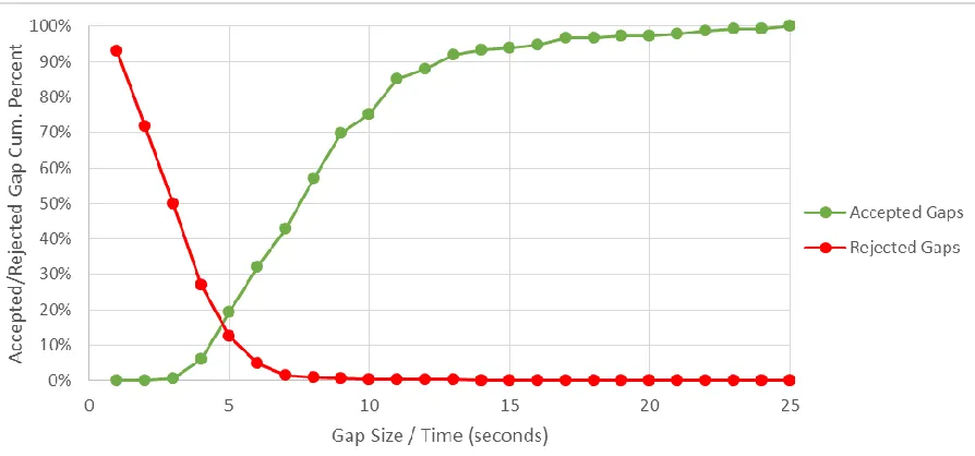
The graphical method for pedestrian gap acceptance uses all of the rejected gaps and
accepted gaps, rather than only being able to use paired observations (Chae, 2005). Rejected gaps and accepted gaps are plotted by gap size and cumulative distribution of the gaps. The critical gap is the intersection of these two probability plots, where the probability of accepting a gap is the same as rejecting a gap. Results are easily biased and provide approximate results.
Methods for vehicular gap acceptance typically include the concept of follow-up time. Follow-up time is not considered for pedestrians since they are not required to wait in a single queue as vehicles do, but can instead cross together in an acceptable gap (Schroeder, 2008). The HCM (2010) includes calculations for the spatial distribution of pedestrians and the group critical headway.
2.4 Yield Behavior
The decision of a driver to yield or of the pedestrian to GO is generally dependent on the following classes of variables: vehicle dynamics, driver characteristics, pedestrian
opposing direction or adjacent travel lane. Yielding behavior is also intuitively related to whether or not a vehicle is traveling in a platoon of vehicles. Other factors may include the cross-section of the road, the type of crossing treatment or the general level of congestion at the crossing location.
The rate of driver yielding to pedestrians at unsignalized crosswalks varies across locations (Rodegerdts, 2007), but in nearly all cases is less than 100%. Findings from NCHRP report 572 (Rodegerdts, 2007) show that 43% of the drivers at two-lane approaches of the
roundabout do not yield to pedestrians. The lack of yielding is only 17% for single-lane roundabouts. It can be said that the number of lanes affect driver yielding, at least for
roundabouts. Fitzpatrick (2006) noted that certain roadway design elements, such as number of through lanes and posted speed limit, have a significant impact on driver yielding at unsignalized midblock crossings. Motorists are also more likely to yield on narrow, low-volume roadways.
Figure 1: Yielding Rates for Various Crossing Treatments (TRB, 2010)
In previous research, Sun, et al. (2002) collected data on driver yielding and pedestrian gap acceptance at an unsignalized midblock pedestrian crossing. They found that drivers are more likely to yield to a group of pedestrians and that older drivers were more likely to yield than younger drivers. The authors looked at only one crosswalk and did not analyze any pedestrian treatment effects. The authors collected 1.5 hours of each AM and PM peak data over 5 days, for a total of 15 hours of data. The resulting samples included 687 accepted gap, 938 rejected gap and 1254 motorist yield data points.
A study by Salamati, et al. (2012) showed that the drivers tend to yield to pedestrians with white canes more often than sighted pedestrians. Drivers traveling in the far lane, relative to pedestrian location, have lower probability of yielding to a pedestrian than drivers in the near lane. As the speed increases the probability of driver yielding decreases. The results show that factors such as vehicle platooning, downstream conflict and pedestrian waiting position do not have a significant impact on the probability of a driver yielding to a pedestrian. 2.5 Highway Capacity Manual 2010 Pedestrian Delay Estimation
In chapter 19 of HCM 2010, pedestrian level of service (LOS) at two-way stop-controlled intersections (TWSC) is defined for pedestrians crossing the traffic stream not controlled by a STOP sign (TRB, 2010). This method can be applied to midblock pedestrian crossings. LOS is determined by computed or measured control delay, where extremely long delays result in LOS F. The pedestrian methodologies were developed separately from the vehicle methodology and have different limitations. These pedestrian methodologies apply to TWSC intersections and midblock crossings where up to four through lanes can be crossed, or eight through lanes if a center median is provided for refuge. It is assumed that the crosswalk is isolated, away from signals.
The TWSC intersection methodology for the pedestrian mode is applied through a series of steps requiring input data related to vehicle and pedestrian volumes, geometric conditions, and motorist yield rates to pedestrians to calculate the average pedestrian delay. The following six steps are required:
(1) Identify two-stage crossings, (2) Determine critical headway,
(6) Calculate average pedestrian delay and determine LOS
Pedestrians typically cross in two stages when a refuge is provided. Pedestrian delay should be estimated for each stage of crossing and summed to establish average delay for entire crossing (TRB, 2010).
Critical gap, or headway, is then estimated, which is the minimum average gap length accepted by half of all pedestrians. The critical headway for a single pedestrian (tc, seconds)
depends on the crosswalk length (L, feet), average pedestrian walking speed (Sp, ft/s), and
pedestrian start-up time and end clearance time (ts, seconds) (TRB, 2010). The equation is
shown below. Rouphail, et al. (2005) described pedestrian gap acceptance as the sum of latency and actual crossing times, an approach similar to the HCM 2010 method discussed above. Field estimates of latency time could be used in place of the HCM 2010 start-up time.
s p
c t
S L
t (1)
The group critical headway (tc,G, seconds) calculation requires that the spatial distribution of
pedestrians (Np, pedestrians) be calculated from the total number of pedestrians in the
crossing platoon (Nc, pedestrians). Equations for group critical headway, spatial distribution
of pedestrians, and total number of pedestrians in the crossing platoon are provided below (TRB, 2010):
𝑡𝑐,𝐺 = 𝑡𝑐+ 2(𝑁𝑝− 1) (2)
𝑁𝑝 = 𝐼𝑛𝑡 [
8.0(𝑁𝑐−1)
𝑊𝑐 ] + 1 (3)
𝑁𝑐 =
𝑣𝑝𝑒𝑣𝑝𝑡𝑐+𝑣𝑒−𝑣𝑡𝑐
(𝑣𝑝+𝑣)𝑒(𝑣𝑝−𝑣)𝑡𝑐
(4)
Wc= Crosswalk Width (ft)
vp = Pedestrian Flow Rate (ped/s)
v = Vehicular Flow Rate (veh/s)
Probability of a pedestrian not incurring a delayed crossing is equal to the likelihood that a pedestrian will encounter a gap greater than or equal to the critical headway immediately upon arriving at the intersection. This probability can be estimated using a Poisson
distribution and assuming random arrivals of vehicles. The probability of a blocked lane (Pb),
gap not exceeding critical headway, is the complement. Probability of a delayed crossing (Pd), assuming independent distribution of traffic in each through lane, is a function of the
blocked lane probability and the number of through lanes crossed (L) (TRB, 2010).
𝑃𝑏 = 1 − 𝑒−𝑡𝑐,𝐺𝑣𝐿 (5)
𝑃𝑑 = 1 − (1 − 𝑃𝑏)𝐿 (6)
The average delay to a pedestrian waiting for an adequate gap at an unsignalized crossing, assuming no driver yielding, depends on the critical headway and vehicular flow rate.
Average gap delay for pedestrians who incur nonzero delay (dgd, seconds) is a function of the
probability of a delayed crossing and the average pedestrian gap delay (dg, seconds). Both
equations are given below (TRB, 2010): 𝑑𝑔 =1
𝑣(𝑒
𝑣𝑡𝑐,𝐺− 𝑣𝑡
𝑐,𝐺− 1) (7)
𝑑𝑔𝑑= 𝑑𝑔
𝑃𝑑 (8)
For any yielding event, each through lane is either clear or blocked. If the lane is clear or the driver in the blocked lane chooses to yield, the pedestrian may cross. Otherwise, the
pedestrian will receive an adequate gap in traffic and will be able to cross without having to depend on yielding motorists. The equation below shows the calculation for average
pedestrian delay (dp, seconds), where the first term represents the delay in waiting for a yield,
the second term represents the delay in waiting for an adequate gap, and the third term represents the adjustment to delay in the event of a driver yielding (TRB, 2010):
𝑑𝑝 = (∑𝑛𝑖=1ℎ(𝑖 − 0.5)𝑃(𝑌𝑖)) + 𝑑𝑔− 𝑑𝑔𝑑∑𝑛𝑖=1𝑃(𝑌𝑖) (9)
Where: i = Crossing Event (i = 1 to n)
h = Average Headway for each through lane
P(Yi) = Probability that motorists yield to pedestrian on crossing event i
n = Int(dgd/h), average number of events before an adequate gap is available
The probability that a driver will yield for a given crossing event are provided with models for each of one, two, three, and four lane crossings. The equation is simplest when the pedestrian is crossing one through lane and is provided below for any crossing event:
𝑃(𝑌𝑖) = 𝑃𝑑𝑀𝑦(1 − 𝑀𝑦) 𝑖−1
(10)
Where: My = Motorist Yield Rate (decimal)
The motorist yield rate in the HCM can be obtained from Exhibit 19-17, which is replicated above as Figure 1. However, that exhibit only shows average yield rates for some treatments, and is not sensitive to crosswalk geometry or behavioral attributes. No method or equation exists in the HCM to estimate My, short of field measurements.
𝑃(𝑌𝑖) = [𝑃𝑑 − ∑𝑖−1𝑗=0𝑃(𝑌𝑗)] [(2𝑃𝑏(1−𝑃𝑏)𝑀𝑦)+(𝑃𝑏2𝑀𝑦2)
𝑃𝑑 ] (11)
𝑃(𝑌𝑖) = [𝑃𝑑 − ∑𝑖−1𝑗=0𝑃(𝑌𝑗)] [
𝑃𝑏3𝑀𝑦3+3𝑃𝑏2(1−𝑃𝑏)𝑀𝑦2+3𝑃𝑏(1−𝑃𝑏)2𝑀𝑦
𝑃𝑑 ] (12)
𝑃(𝑌𝑖) = [𝑃𝑑− ∑𝑖−1𝑗=0𝑃(𝑌𝑗)] [
𝑃𝑏4𝑀𝑦4+4𝑃𝑏3(1−𝑃𝑏)𝑀𝑦3+6𝑃𝑏2(1−𝑃𝑏)2𝑀𝑦2+4𝑃𝑏(1−𝑃𝑏3)𝑀𝑦
𝑃𝑑 ] (13)
The final step in the HCM method is to calculate the average pedestrian delay, the service measure, and determine the LOS. For two-stage crossings, the pedestrian delay is equal to the sum of the delay for each stage of the crossing (TRB, 2010).
2.6 Mixed-Priority Pedestrian Delay Models
Schroeder and Rouphail (2010) developed mixed-priority pedestrian delay models at single-lane roundabouts by using behavioral crossing data. “Mixed-priority” refers to crosswalk operations where drivers at times yield to create crossing opportunities, but sometimes pedestrians need to rely on their own judgment of gaps in traffic to safely cross the street. Probabilistic behavioral parameters were measured for controlled crossings by blind pedestrians. The delay model is designed to apply to any pedestrian population, where perfect utilization can be assumed for sighted pedestrians. Delay is predicted as a function of the following probabilities: encountering a crossing opportunity in the form of a yield or crossable gap and utilization of said yield or gap, with these factors being combined to produce an overall probability of crossing. A multi-linear, log-transformed regression approach was used to predict the average pedestrian delay. The variables were transformed by applying the natural logarithm because the delay distribution suggested a log-normal distribution by being skewed to the left. The resulting model was statistically significant and produced good estimates of pedestrian delay that matched the observed field data.
applicable where pedestrian delay is determined by a mix of pedestrian gap acceptance and driver yielding behavior. The following variables were calculated and considered for model development: probability a vehicle would yield to the pedestrian, probability a yield event is encountered, probability of yield utilization, probability of a gap being crossable, probability of encountering a crossable gap, observed delay per leg, minimum delay, probability of crossing in a yield, probability of crossing in a crossable gap, probability of crossing. The final model was determined by significant parameter estimates, a high adjusted R2 value, and relatively simple and practical model form. Pedestrian delay was predicted as a function of P(Cross), the overall probability of crossing calculated from the four individual probability parameters, for the recommended model, shown below (Schroeder and Rouphail 2010):
𝑑𝑝 = −0.78 − 14.99ln(𝑃cross) (14)
Where: dp = average pedestrian delay (seconds)
ln = natural logarithm
Pcross = probability of crossing = P(Y_and_GO) + P(CG_and_GO)
= P(Y_ENC)*P(GO|Y) + P(CG_ENC)*P(GO|CG) P(Y_and_GO) = probability of crossing in a yield
P(CG_and_GO) = probability of crossing in a crossable gap (CG) P(Y_ENC) = probability of encountering a yield event
P(GO|Y) = probability of yield utilization
P(CG_ENC) = probability of encountering a CG event P(GO|CG) = probability of crossing in a critical gap
pedestrians. P(Y_ENC), P(GO|Y), P(CG_ENC), and P(GO|CG) need to be field-measured or derived from literature, previous studies, and traffic theory. Average pedestrian delay of sighted pedestrians can be determined by assuming perfect opportunity utilization.
Utilization rates for blind pedestrians and other special populations, such as children and the elderly, will be lower and requires judgment by the analyst. Rate of driver yielding, P(Yield), can be measured in the field using manual tally and stop-watch methods. In the absence of field data, results from past studies can be used as guidance. The probability of encountering a yielding vehicle (P(Y_ENC)) better represents the flow rate that the pedestrian is likely to experience, since it is calculated from all encountered vehicles rather than those that could have yielded. The equation for estimating P(Y_ENC) is provided below (Schroeder, et al. 2011):
𝑃(Y_ENC) = 𝑃(Yield) ∗ (100% − 𝑃(CG_ENC)) (15)
Availability of crossable gaps can be field-measured or estimated using traffic flow theory concepts on the basis of traffic volume and an assumed headway distribution. May (1990) used a simple negative exponential distribution to determine the probability of observing a headway greater than the critical headway (tc, seconds) calculated using HCM methods,
which is the probability of encountering a crossable gap (P(CG_ENC)). The equation is provided below (Schroeder and Rouphail, 2010):
𝑃(CG_ENC) = 𝑃(ℎ𝑒𝑎𝑑𝑤𝑎𝑦 ≥ 𝑡𝑐) = 𝑒
𝑡𝑐
𝑡𝑎𝑣𝑔 (16)
Where: tavg = average headway, (3600 s/h)/(vehicles/h) 2.7 Limitations of Current Pedestrian Delay Models
was developed using field data, but the data was only collected for controlled blind pedestrian crossings at single-lane roundabouts (Schroeder and Rouphail, 2010). Driver yielding rates for various crossing treatments from data collected for staged (controlled) and unstaged pedestrians are provided in the HCM 2010. These values were found from a limited number of sites and all available treatments are not covered. Local knowledge and
engineering should be used to supplement these values.
3.
METHODOLOGY
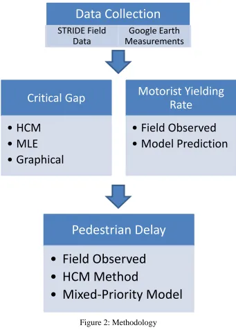
Figure 2: Methodology
The HCM 2010 method and the mixed-priority pedestrian delay model both require certain input data. Observational data on pedestrian-vehicle interaction was collected at the event level for midblock pedestrian crossings. Event level in this context refers to the interaction of one vehicle and one pedestrian. Vehicle volumes will be collected rather than assuming equal
Data Collection
STRIDE Field
Data
Google Earth
Measurements
Critical Gap
• HCM
• MLE
• Graphical
Motorist Yielding
Rate
• Field Observed
• Model Prediction
Pedestrian Delay
• Field Observed
• HCM Method
directional distribution by drivers at two-stage crosswalks. Non-yielding platooned vehicles will be accounted for in longer field delays. Driver yielding behavior and pedestrian gap acceptance may vary significantly at locations with varying land use and facility designs. In order to achieve greater heterogeneity in the study, various unsignalized midblock crossing locations were considered for the observational studies with varying pedestrian treatments, lane configurations, built-up environment, and travel activity from Alabama, Florida, and North Carolina. At sites with limited pedestrian activity, controlled experiments were performed. A total of 27 sites were selected for data collection.
The following definitions will be used through the remainder of the thesis: Event: The interaction of one vehicle and one pedestrian.
Yield: A driver either coming to a complete stop or slowing down to create a crossing opportunity for the pedestrian(s)
Gap: Time (in seconds) between two successive vehicle arrivals (front bumper to front bumper)
Lag: Time (in seconds) between the pedestrian arrival at the crosswalk and the arrival of the first vehicle measured in seconds. For analysis purposes, lags were considered to be accepted/rejected gaps
Critical Gap/Headway: Minimum average gap length accepted by half of all pedestrians to safely cross the street.
3.1 Data Needs for Analysis Methods
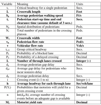
Table 1: HCM Pedestrian Delay Method Inputs
Variable Meaning Units
tc Critical headway for a single pedestrian Secs.
L Crosswalk length Feet
Sp Average pedestrian walking speed Ft/s
ts Pedestrian start-up time and end
clearance time (assume default of 3 secs.)
Secs.
Np Spatial distribution of pedestrians Peds.
Nc Total number of pedestrians in the crossing
platoon
Peds.
Wc Crosswalk width Feet
vp Pedestrian flow rate Ped/s
v Vehicular flow rate Veh/s
tc,G Group critical headway Secs.
Pb Probability of a blocked lane Decimal
Pd Probability of a delayed crossing Decimal
L Number of through lanes crossed Integer (+)
dg Average pedestrian gap delay Secs.
dgd Average gap delay for pedestrians who
incur nonzero delay
Secs.
dp Average pedestrian delay Secs.
i Crossing event (i=1 to n) Integer (+)
h Average headway for each through lane Sec/veh/lane
P(Yi) Probabilities that motorists will yield for a
given crossing event
Decimal
n Int(dgd/h), average number of crossing
events before an adequate gap is available
Integer (+)
My Motorist yield rate Decimal
increases. Maximum likelihood estimation and the graphical method will also be used to determine the critical gap from rejected and accepted gaps.
The mixed-priority pedestrian delay model requires the calculation of several probabilities; including encountering a yield, yield utilization, encountering a crossable gap, and gap utilization. These probabilities are used to calculate the probability of crossing. Probability of yield utilization was assumed to be 100%, which is a reasonable assumption when all
pedestrians are sighted. Number and size of rejected gaps, critical gap, and whether the pedestrian crossed in a gap or yield are required to calculate the other probabilities. Other variables will be needed to develop an improved driver yielding model for the estimation of pedestrian delay. Number of lanes, crossing width, traffic volume, pedestrian volume, treatment in place, whether the site is one-way or two-way, on-campus or off-campus, and which state the site is located in will be used to develop the improved model.
3.2 Field Data Collection
The data collection methodology to evaluate the interaction of pedestrians and drivers at midblock pedestrian crossings at a microscopic or event level was borrowed from previous research by Schroeder (2008). Accepted and rejected gap sizes, pedestrian walking speed, observed pedestrian delay, and driver decision will be gathered from individual observations. Percentage of driver yielding and average pedestrian delay can be determined from the data. The data collection effort was performed in conjunction with a Southeastern Transportation Research, Innovation, Development and Education Center research project (STRIDE 2012-016S). A variety of empirical data on pedestrian-vehicle interaction was collected using observational studies. These variables must be collected accurately using reliable
assumption is made that both the driver and pedestrian are consciously aware of each other’s presence.
A three-pronged data collection approach that combined real-time observations by a trained observer on a tally sheet, video recording of the crosswalk, and LIDAR speed measurements of approaching vehicles was used. Multiple hours of observations were taken at each site. The LIDAR was used to record the speed and distance of the approaching vehicle once the pedestrian (waiting at the curb or in the crosswalk) entered the view of the driver. A video camera was set up on a tripod to capture the pedestrian-vehicle interactions so that the researchers could gather some data at a later point, rather than having to quickly gather everything immediately. The researcher taking the speed and distance measurements would read these values out loud, so that the interaction could be quickly identified in the video. Figure 3 shows a schematic of the data collection set-up.
Figure 3: Field Data Collection Set-Up
In order to capture all relevant data, the video angle has to cover events concurrent to the interaction, such as the presence of multiple pedestrians. As shown in the diagram, the video camera angle is wide enough to cover the crosswalk influence area (CIA) or waiting location, and the approach to the crosswalk.
Site visits and/or using Google Earth served as a starting point to collect basic information about potential sites. A few sites generated little naturally occurring pedestrian interactions
with vehicular movements. Controlled experiments comprising of staged crossings by research members while another member recorded detailed vehicular data were used at such locations to obtain pedestrian-vehicle interactions.
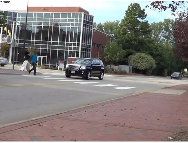
A total of 27 sites were selected for data collection and analysis (9 in Alabama, 10 in Florida, and 8 in North Carolina), where 11 of the sites were at university on-campus locations. An example of a study site from North Carolina is depicted in Figure 4. Posted speeds at these locations ranged from 15 mph to 40 mph. Single lane and multilane configurations were used. Some of the sites also had bike lanes and on-street parking.
Figure 4: Example of Study Site and Data Collection Setup
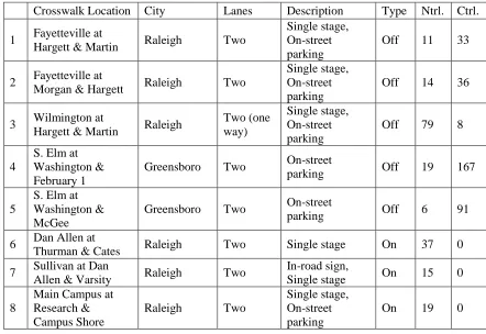
Table 2: Data Collection Sites in North Carolina
Crosswalk Location City Lanes Description Type Ntrl. Ctrl.
1 Fayetteville at
Hargett & Martin Raleigh Two
Single stage, On-street parking
Off 11 33
2 Fayetteville at
Morgan & Hargett Raleigh Two
Single stage, On-street parking
Off 14 36
3 Wilmington at
Hargett & Martin Raleigh
Two (one way)
Single stage, On-street parking
Off 79 8
4
S. Elm at Washington & February 1
Greensboro Two On-street
parking Off 19 167
5
S. Elm at Washington & McGee
Greensboro Two On-street
parking Off 6 91
6 Dan Allen at
Thurman & Cates Raleigh Two Single stage On 37 0
7 Sullivan at Dan
Allen & Varsity Raleigh Two
In-road sign,
Single stage On 15 0
8
Main Campus at Research & Campus Shore
Raleigh Two
Single stage, On-street parking
Table 3: Data Collection Sites in Florida
Crosswalk Location City Lanes Description Type Ntrl. Ctrl.
1 Gale Lemerand Dr. Gainesville Two
Flashing pedestrian sign, Bike lanes
On 35 82
2
Museum Rd. & Fraternity Row (EB)
Gainesville Two Single stage,
Bike lanes On 0 45
3
Museum Rd .& Fraternity Row (WB)
Gainesville Two Single stage,
Bike lanes On 0 47
4 Museum Rd. &
Reitz Union Dr. Gainesville Two
Ped sign, Single
stage, Bike lanes On 30 0
5 Hull Rd. Gainesville Two Single stage,
Bike lanes On 42 0
6 Museum Rd. & SW
13th St. Gainesville Two
Ped sign, Bike
lanes On 38 0
7 SW 2nd Ave. &
SW 8th St. Gainesville Two
In-road sign, On-street parking, Bike lanes
Off 1 21
8 SW 2nd Ave. &
SW 3rd St. Gainesville Two
In-road sign, On-street parking, Bike lanes
Off 0 29
9 SE 2nd Ave. & SE
6th St. Gainesville Two
Single stage, On-street parking, Bike lanes
Off 0 27
10 SW 2nd Ave. &
SW 1st St. Gainesville Two
In-road sign, On-street parking, Bike lanes
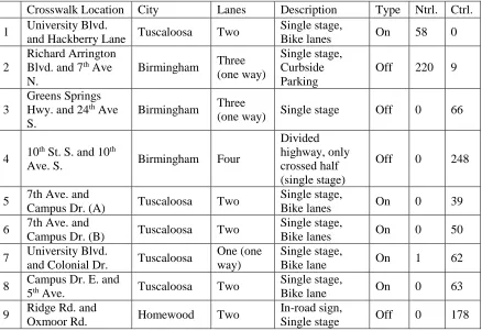
Table 4: Data Collection Sites in Alabama
Crosswalk Location City Lanes Description Type Ntrl. Ctrl.
1 University Blvd.
and Hackberry Lane Tuscaloosa Two
Single stage,
Bike lanes On 58 0
2
Richard Arrington Blvd. and 7th Ave
N.
Birmingham Three (one way)
Single stage, Curbside Parking
Off 220 9
3
Greens Springs Hwy. and 24th Ave
S.
Birmingham Three
(one way) Single stage Off 0 66
4 10
th St. S. and 10th
Ave. S. Birmingham Four
Divided highway, only crossed half (single stage)
Off 0 248
5 7th Ave. and
Campus Dr. (A) Tuscaloosa Two
Single stage,
Bike lanes On 0 39
6 7th Ave. and
Campus Dr. (B) Tuscaloosa Two
Single stage,
Bike lanes On 0 50
7 University Blvd.
and Colonial Dr. Tuscaloosa
One (one way)
Single stage,
Bike lane On 1 62
8 Campus Dr. E. and
5th Ave. Tuscaloosa Two
Single stage,
Bike lane On 0 63
9 Ridge Rd. and
Oxmoor Rd. Homewood Two
In-road sign,
Table 5 summarizes all data collection elements used in pedestrian delay estimation by the HCM method and the mixed-priority method.
Table 5: Data Collection for Pedestrian Delay Estimation
Factor Description Value
Fir st V eh ic le Va ri abl es SPD
The speed of the first vehicle (mph), at the time the pedestrian arrives at crosswalk influence area (waiting location), recorded from speed gun
Mph
DIST The distance from the first vehicle to the researcher
recorded from the laser speed gun Ft
Y_NY Whether the first vehicle yielded or not Yield=1, Non-yield=0
TRIG
If the first vehicle yielded, was it triggered (forced) by the pedestrian. In other words, if the yield happened before pedestrian stepping into the crosswalk (0) or after (1)
Triggered Yield, Yes=1, No=0
STP
Whether the first vehicle had already stopped at the time that the pedestrian arrived. Observations where the vehicle was previously stopped were removed.
Stopped=1
DIST_DEL Delay between when speed should have been taken (at time pedestrian arrives at CIA) and when gun beeped Seconds
ADJDIST
Vehicle position at time of pedestrian arrival in CIA measured using LIDAR speed measurement device; ADJDIST calculated from measured distance, speed, distance delay and Distance to Crosswalk; ADJDIST= DIST+SPD*1.467*DIST_DEL-Distance to Crosswalk
Ft Pedes tr ian Va ri abl es
CTRL Whether crossing pedestrian was controlled (researcher) or random (observational study) Controlled=1, Random=0
CROSS Whether pedestrian crossed in a gap or a yield Gap/Yield (G/Y)
TIME
Time from pedestrian stepping into crosswalk to reaching measured location (such as specific white crosswalk marking, center line, or opposite side of crosswalk). Used in calculating pedestrian walking speed.
Seconds
W_SP Pedestrian walking speed while crossing;
W_SP=Crossing Distance/TIME Ft/s
GAP Observed lag or gap time, calculated from SPD and ADJDIST Seconds
REJ1 – REJ15 Rejected gap sizes Seconds
MAX REJ The largest rejected gap for a single pedestrian
(maximum value of REJ1 – REJ15) Seconds
Table 5 Continued
Factor Description Value
DELAY Time from the pedestrian arriving at the crosswalk influence area (waiting location) to stepping into the crosswalk to cross
Seconds Sit e V ar iab les Distance to Crosswalk
The distance from the researcher using the laser speed
gun to the middle of the crosswalk along the curb. Ft
Crossing Distance
The distance from the curb to a measured location, such as a specific white crosswalk marking, a center line, or the opposite side of the crosswalk.
Ft
Crosswalk Length
Equivalent to lane width multiplied by the number of through lanes for each stage of crossing measured from Google Earth
Ft
Crosswalk
Width Width of the crosswalk measured from Google Earth Ft My Observed motorist yield rate Decimal
O
ther COUNT If the first vehicle did not yield, how many vehicles went
through before the pedestrian crossed Number
V
ideo
vp Pedestrian flow rate Peds/s
v Vehicular flow rate Peds/s
Free-flow speed was found by averaging a sample of unimpeded vehicle speeds for each site. For sites where the free-flow speed was not reported, speed limit was used. Pedestrian and vehicular flow rates were found either in the field or from the video at a later point in time. The crosswalk lengths used will not include on-street parking, bike lanes, or median refuges. 3.3 Analysis Methods
crossings. The next step is to determine the critical headway and group critical headway for sites with pedestrian pooling. Walking speeds were averaged for each site and then used to find the critical headway for the HCM method of determining critical gap (seen in Equation 1). Maximum likelihood estimation and the graphical method were also used and the results compared in Chapter 5. If the value for the rejected gap or accepted gap size is not provided, values of “3” and “30” were respectively used. Group critical headway was calculated from Equation 2 using the critical headway for a single pedestrian and the spatial distribution of pedestrians, which was calculated from Equation 3 and Equation 4.
Only observations with rejected and accepted gaps can be used in maximum likelihood estimation. The accepted gap and the largest rejected gap for each observation are entered into the spreadsheet created by Troutbeck (1992). A visual basic code then runs through as many iterations as are necessary to converge on a single value. This value is taken to be the average for all pedestrians observed. Observations with very large accepted gaps may need to be removed. The threshold to determine what is considered “large” will be decided during data analysis. Sample sizes for this method are greatly reduced, since only paired
observations could be used and large values had to be removed. Other methods may provide more accurate results from the larger sample sizes. Sites are segregated by crossing lengths into three groups, 30+ feet, 15 ‒ <30 feet, and <15 feet crossing lengths. It is assumed that critical gaps for sites within each group would be similar since crossing time is strongly dependent on the length of the crosswalk. The graphical method used all of the rejected gaps and accepted gaps. Distributions were created for the three groups identified above. The intersection of distributions for each graph is taken as the critical gap for the sites in the grouping. This method is easily biased by outliers, so “large” values were removed. Other critical gap methods, such as Ramsey-Routledge method, could also have been used. For the purpose of this research, the number of methods was limited to three.
(Equation 5) and the number of through lanes crossed. The fourth step is to calculate the average delay to wait for an adequate gap (Equation 7) and the fifth step is to estimate the delay reduction due to yielding vehicles (third term of Equation 9). The final step is to calculate the average pedestrian delay (Equation 9) from the delay in waiting for a yield, delay in waiting for an adequate gap, and the adjustment to delay in the event of a driver deciding to yield. Delays related to driver yielding rely on P(Yi), the probability that
motorists yield to the pedestrian on a particular crossing event i. Equations 10, 11, and 12 calculate this probability at one-, two-, and three-lane crossings, respectively. The probability of a blocked lane, probability of a delayed crossing, and motorist yield rate are used to
calculate P(Yi). Motorist yield rates were found for each site by taking the number of
motorists who yielded divided by the number of events and will also be predicted by a regression model developed in this thesis. These two values will be compared to test the validity of the regression model.
number of crossable gaps if the pedestrian was able to cross in a gap (number of rejected and accepted gaps greater than the critical gap). For average pedestrian delay at each site, where each site represents a data point, these probabilities are averaged before calculating P(Cross). Average pedestrian delay will be estimated from the HCM method and mixed-priority
method using three different critical gap values and two different values for motorist yielding rate for each site. This will result in twelve values for average pedestrian delay per site. These estimates will be compared to the observed average pedestrian delay. Pedestrian delay may vary between methods for estimation and critical gap values used.
3.4 Statistical Models
Mean yield rates are given for several crossing treatments, such as overhead flashing
beacons, high-visibility signs, and rectangular rapid-flashing beacons, in the HCM pedestrian delay method. For the mixed-priority pedestrian delay model, the probability of encountering a yield event was defined at a microscopic scale as the number of yields divided by the total number of events encountered by a pedestrian. Only a few sites were studied for each of these methods. It is recommended that practitioners supplement mean yield rates with local knowledge and engineering judgment.
Regression models will be used to predict motorist yield rate (My) based on several explanatory variables. The model will be validated by comparing the predicted yield rates with the observed rates. For pedestrian delay, the observed and predicted yielding rates will be entered into the HCM method and mixed-priority models and then be compared to the field estimated delay.
Table 6 summarizes all variables considered for model development. This includes the expected impact of the variable on driver yielding, where “+” represents that higher or true values are expected to increase the chance of driver yielding and “‒” represents the
Table 6: Variables Considered for Driver Yielding Model
Variable Description Value
Anticipated Effect on Yielding
CAMPUS This variable distinguishes sites on-campus
(1) from those off-campus (0) On-Campus=1 +
FLORIDA
This variable distinguishes sites in the state of Florida (1) from those in the other two states (0)
Florida=1 +
NCAROLINA
This variable distinguishes sites in the state of North Carolina (1) from those in the other two states (0)
North
Carolina=1 ‒
TREATMENT Whether a treatment was present Treatment=1 +
TWO_WAY Whether the road was two-way (bidirectional)
or one-way Two-Way=1 +
TWOLANE Whether the site had two lanes Two Lanes=1, One=0, Three=0 +
TWOSTAGE
Whether the pedestrian crossing could be completed in two stages (median or pedestrian refuge) or had to be completed in a single stage
Two-Stage=1, Single=0 ‒
PARKING Denotes presence of on-street parking Present=1 + BIKELANE Denotes presence of bike lane(s) Present=1 +
L_WIDTH Lane width Feet ‒
C_WIDTH Crosswalk width Feet ‒
SPEED Free-flow speed (if available) or speed limit
on the roadway Mph ‒
PED_RATE Total pedestrian flow rate Ped/hr + VEH_RATE Total vehicular flow rate (all lanes, directions
summed) Veh/hr ‒
4.
YIELDING MODEL DEVELOPMENT
Multiple linear regression is used to develop a model for predicting driver yielding rates at individual sites. This type of regression shows the linear effects of independent variables on a continuous dependent variable (Moore, 2013). The general linear model is provided below in equation 17. Interaction terms of independent variables could also be used in model
development, but were not considered as part of this research. Simple statistics and variable relationships, such as correlation, should be determined as an early step in the modeling process. Several potential models are created using SAS in order to determine a best fit final regression model, with variables included based on personal observations and statistical significance. The final step is to ensure that model assumptions are met.
𝑦 = 𝛽0+ 𝛽1𝑥1+ 𝛽2𝑥2… + 𝛽𝑘𝑥𝑘+ 𝜀 (17)
Where: y = dependent variable β0 = intercept value
β = coefficients of independent variables x = independent variables
ε = random error
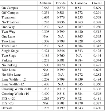
site characteristics. On-campus sites were shown to have higher rates than off-campus sites for each state. The effects of treatment, parking, and crossing width varied from state to state.
Table 7: Observed Motorist Yielding Rates
Figure 5: Motorist Yielding Rates by State and Other Site Characteristics
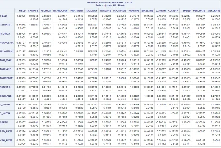
Table 8 shows the correlation coefficients and significance levels between all variables. The following independent variables are positively correlated to the dependent variable,
Table 6 shows that most variables affect yielding as expected, excluding TWO_STAGE, PARKING, and C_WIDTH. CAMPUS, FLORIDA, TWO_WAY, BIKELANE, and
L_WIDTH were each seen to have a significant impact on driver yielding as evident by low p-values. It is expected that these variables will show up in many of the potential models. The high number of significant correlation coefficients shows that the yielding decision relies on several factors, rather than being the result of any single variable.
Table 8: Correlation Table
(-0.70960), NCAROLINA to BIKELANE (-0.72548), and TWO_WAY to TWOLANE (0.74162).
Several multiple linear regression models were then created to predict the likelihood of yielding, represented by the dependent variable YIELD. Several variable selection processes are used (SAS, 2011):
Full Model – uses all independent variables regardless of their p-value.
Forward selection – successively adds variables to the model at a p<0.05 inclusion threshold.
Backward elimination – starts with a full model and then removes variables starting with the highest p-value, until all remaining variables are at p<0.05.
Max R2 ‒ forward selection to fit the best one-variable model, the best two-variable model, and so on, where variables are switched so that R2 is maximized.
Manual selection – a custom model that is informed by the first four modeling results, but considers practical significance (as opposed to just being motivated by statistical fit).
The full model was used to determine which variables were significant and to what extent they were significant when compared to the other variables. It is expected that variables seen as significant in the correlation table will also be significant in the full model. Results for forward selection and backward elimination processes should result in similar models, but may produce slightly different results, especially when independent variables are
additional variables, and is thus a better measure for models with many independent variables.
PROC REG and PROC GLM were used for the full model. Both of these procedures provided the same results, so PROC REG is used for the other potential models. The full model showed that when all of the variables are used, none of them are significant at the p<0.05 level. Forward selection showed only CAMPUS and FLORIDA to be significant (both with p-values of <0.0001). Backward elimination and the best two-variable model (max R-squared method) were identical to the forward selection model. The three- and
four-variable models found using the max R-squared method included four-variables with p-values < 0.15. Specifically, both models included CAMPUS, FLORIDA, and C_WIDTH, and the four-variable model also included TWO_WAY. Models with five variables and more included at least one variable with a p-value > 0.15, so these models were not explored any further. The five-variable model included the same variables as the four-variable model, with the addition of TWOSTAGE. The six-variable included the same with the addition of
PED_RATE. Statistics for the potential models are shown below in Table 9.
Table 9: Potential Models and Statistics
Model p-value R-squared Adjusted R-squared Full 0.0083 0.8317 0.6353
Forward <0.0001 0.7071 0.6827 Backward <0.0001 0.7071 0.6827 2-variable Max R2 <0.0001 0.7071 0.6827
3-variable Max R2 <0.0001 0.7373 0.7030
4-variable Max R2 <0.0001 0.7682 0.7261
5-variable Max R2 <0.0001 0.7830 0.7313
6-variable Max R2 <0.0001 0.7891 0.7259
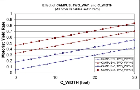
previously mentioned, this model included a variable that was not seen to be significant. The model shows that motorist yielding rate is predicted by CAMPUS, FLORIDA, TWO_WAY, and C_WIDTH.
𝑀𝑦 = 0.04972 + 0.28046𝐶𝐴𝑀𝑃𝑈𝑆 + 0.26527𝐹𝐿𝑂𝑅𝐼𝐷𝐴 + 0.13311𝑇𝑊𝑂_𝑊𝐴𝑌 +
0.01251𝐶_𝑊𝐼𝐷𝑇𝐻 (18)
Figure 6: Model Probability Plots The following assumptions are made in multiple linear regression:
Linearity of the relationships between the dependent and independent variables Independence of the errors
Normally distributed errors
Homoscedasticity, constant error variance
relationships between variables are linear (Washington, et al. 2003). None of the plots displayed curvilinear trends, so the linearity assumption is acceptable.
Individual observations of dependent variables must be independent from each other for the errors to be independent (Washington, et al. 2003). The variables that were seen to be significant for the model are independent of each other, so the error independence
assumption is satisfied. There are several methods to determine if the errors are normally distributed, including histograms and quantile-quantile (Q-Q) plots (Washington, et al. 2003). The histogram for the model will reveal a bell-shaped normal curve and the Q-Q plot will plot a nearly perfect straight line if the errors are normally distributed. It can be seen in Figure 7 below that the errors are normally distributed. Mean squared error, MSE, is used to estimate error variance. MSE will be larger for heteroscedastic regression (Washington, et al. 2003). Since the MSE for this model is 0.0191, it can be said that the model displays
homoscedasticity. All of the assumptions were met, which means that multiple linear regression is an appropriate way to model the data.
5.
DATA ANALYSIS
Results for critical gap, motorist yielding rate, and average pedestrian delay are discussed and compared below.
5.1 Critical Gap 5.1.1 HCM Method
Table 10: Critical Gap from HCM Method Peds. (#) Sp (ft/s) L (ft) tc (sec)
It can be seen that the sites with longer crosswalk lengths have longer critical gaps, which supports the decision to divide the sites into groups based on crosswalk length for maximum likelihood estimation and the graphical method. The groups are as follows:
30 + feet: NC1, NC2, NC3, UAB2, and UAB9
15 ‒ < 30 feet: NC6, NC7, NC8, UF2, UF3, UF4, UF5, UF9, UAB1, UAB3, UAB4, UAB5, UAB6, UAB7, and UAB8
< 15 feet: NC4, NC5, UF1, UF6, UF7, UF8, and UF10
5.1.2 Maximum Likelihood Estimation
times the required crossing time were removed resulting in a sample size of 41 pairs and a critical gap of 6.252 seconds.
5.1.3 Graphical Method
All rejected gap values are used for the graphical method, not just the maximum rejected gap. The distributions of rejected and accepted gaps were plotted and the intersection was taken to be the critical gap. Accepted gap values greater than three times the required crossing time were removed for all groups, leaving the following sample sizes:
30 + feet: 139 accepted gaps and 388 rejected gaps 15 ‒ < 30 feet: 149 accepted gaps and 423 rejected gaps < 15 feet: 99 accepted gaps and 285 rejected gaps
Figure 8 below shows the full graph for the “15 ‒ <30 feet” group and Figure 9 shows close-up views of the intersections for each groclose-up.
(a) “30 +” (b) “15 ‒ < 30” (c) “< 15” Figure 9: Graphical Method Close-ups
It can be seen that the critical gap is approximately 5.365 seconds for the “30 +” group, 4.750 for the “15 ‒ < 30” group, and 4.635 for the “< 15” group.
5.1.4 Comparison
Table 11: Critical Gap Values by Site and Method Site tc (HCM) tc (MLE) tc (GM)
NC1 9.911 6.764 5.365 NC2 9.911 6.764 5.365 NC3 11.750 6.764 5.365 NC4 5.597 6.252 4.635 NC5 5.575 6.252 4.635 NC6 8.303 6.339 4.750 NC7 7.000 6.339 4.750 NC8 7.861 6.339 4.750 UF1 4.866 6.252 4.635 UF2 6.846 6.339 4.750 UF3 6.656 6.339 4.750 UF4 6.978 6.339 4.750 UF5 7.453 6.339 4.750 UF6 5.227 6.252 4.635 UF7 5.179 6.252 4.635 UF8 4.930 6.252 4.635 UF9 6.269 6.339 4.750 UF10 5.335 6.252 4.635 UAB1 8.778 6.339 4.750 UAB2 10.692 6.764 5.365 UAB3 7.829 6.339 4.750 UAB4 8.485 6.339 4.750 UAB5 8.689 6.339 4.750 UAB6 8.417 6.339 4.750 UAB7 6.542 6.339 4.750 UAB8 9.813 6.339 4.750 UAB9 9.667 6.764 5.365
5.2 Motorist Yield Rate 5.2.1 Observed Yielding Rates
found for groups of sites based on site characteristics, such as campus type, state, and number of lanes.
5.2.2 Driver Yielding Model
Predicted values for each site and various groups were found using a driver yielding model developed in SAS. The model can be seen in chapter 4. The predicted motorist yielding rate is given as a decimal. TWOLANE, TWOSTAGE, PED_RATE, and VEH_RATE were not used in the motorist yielding model, but these variables are used in the HCM pedestrian delay estimation method.
5.2.3 Comparison