Implementation of dynamic synchronization for Slipstream Multiprocessors

Abstract

SIVAGNANAM, SUBHASHINI

Implementation of dynamic synchronization for

Slipstream Multiprocessors

(Under the direction of Dr. Gregory T. Byrd)

The main goal of parallelization is speed up. As the number of processors

increases, there is a little or no speedup, since a performance threshold is reached for a

fixed problem size. This is because scalability for a parallel program is limited by the

communication and synchronization overhead. Slipstream multiprocessor runs two

redundant copies of the same program in a chip multiprocessor, where one program runs

ahead of the other. The leading program is called the A-Stream and the trailing one is the

R-Stream. The A-Stream, which runs ahead, is used to reduce overhead and improve the

efficiency of execution rather than to increase concurrency. Prefetching of shared data by

the A-Stream for the R-Stream helps the whole unit to speedup.

AR-Synchronization limits the movement of the leading program (A-Stream). The

user can choose the type of synchronization desired at the beginning of program

execution. A program might benefit if we vary the synchronization mode with different

regions of code. This thesis proposes a technique to make the synchronization mode

dynamic.

This thesis implements a method to check whether it is possible to change

synchronization method dynamically. This method incurs some overhead which we avoid

when we implement the sliding-window method to eliminate aggressive switching.

Implementation of dynamic synchronization for

Slipstream Multiprocessors

by

Subhashini Sivagnanam

A thesis submitted to the graduate faculty of

North Carolina State University

In partial fulfillment of the requirements of the degree of

Master of Science

COMPUTER ENGINEERING

Raleigh

2003

Approved by

________________________________

Dr. Gregory T. Byrd, Chair of the Advisory Committee

__________________________

_____________________________

BIOGRAPHY

Subhashini Sivagnanam was born on 12

May 1980 in Madras, India. In 2001, she

graduated with a B.E degree in Electronics and Communication Engineering from

University of Madras, India.

Acknowledgements

I am immensely grateful to Dr. Gregory Byrd for having given me this opportunity to

work for him. He has been patient, encouraging and understanding. He was always

available to help me whenever I was stuck while working on this thesis. I would like to

thank him for all the help he has done for me

I would like to thank Dr. Eric Rotenberg for his valuable suggestions and guidance

during the course of this thesis. I think his enthusiasm and energy are infectious.

I also thank Dr. Edward Gehringer for having agreed to be on my thesis committee and

for his valuable comments after reviewing my thesis.

I would like to thank Khaled Ibrahim for being patient and helping me whenever I had

problems with the simulator.

TABLE OF CONTENTS

LIST OF FIGURES ... vi

LIST OF TABLES ... viii

Chapter 1 Introduction ... 1

1.1 Slipstream Multiprocessors... 2

1.2 AR-Synchronization ... 4

1.3 Need for AR-Synchronization ... 5

1.4 Contribution and Organization of Thesis... 6

1.4.1 Contribution ... 6

1.4.2 Organization:... 7

Chapter 2 The Framework: Design and Implementation... 8

2.1 Experimental Setup... 8

2.1.1 Simulation Environment ... 8

2.1.2 Benchmarks... 9

2.2 Methodology... 10

2.2.1 Basis for switching... 10

2.2.2 Trace Formation... 10

2.2.3 Implementation of adaptive algorithm... 12

2.2.4 Results... 14

Chapter 3 Sliding-window method ... 17

3.1 Implementation of the method ... 17

3.2 Results... 19

3.2.1 OCEAN... 19

3.2.2 SOR... 22

3.2.3 MG ... 24

3.3 OCEAN: further study ... 26

Chapter 4 Related Work... 29

Chapter 5 Summary and Future Work ... 31

5.1 Summary... 31

5.2 Future Work ... 32

LIST OF FIGURES

LIST OF TABLES

Table 2-1 Projected Execution Time ...11

Table 3-1 System Specifications...8

Table 3-2 Benchmarks Grid Size...9

Chapter 1

Introduction

The main goal of parallelization is speedup. As the number of processors

increases, there is a little or no speedup, since a performance threshold is reached for

a fixed problem size. This is because scalability for a parallel program is limited by

the communication and synchronization overhead.

Slipstream execution mode [2][3][4] attempts to reduce these overheads and

enhance scalability by using additional computing resources to improve

inter-processor communication. In slipstream mode, a multiinter-processor runs two redundant

copies of the same program in a chip multiprocessor where one program runs ahead of

the other. The leading program is called the Advanced Stream (A-Stream) and the

trailing one is the Redundant Stream (R-Stream). The A-Stream, which runs ahead, is

used to reduce overhead and improve the efficiency of execution rather than to

increase concurrency. Prefetching of shared data by A-Stream for R-Stream helps the

whole unit to speed up.

AR-Synchronization limits the movement of the leading program (A-Stream).

In previous research, the user was only allowed to choose the type of synchronization

desired at the beginning of program execution. A program might benefit if we vary

the synchronization mode for different regions of code. This thesis aims at proposing

1.1 Slipstream Multiprocessors

We consider running slipstream mode on a chip multiprocessor (CMP) based

distributed shared memory multiprocessor with shared L2 cache. Slipstream mode

executes the same task on both the processors, where one processor helps in reducing

the overhead and to improve the overall execution time [3][2]. This approach is

similar to the uniprocessor slipstream paradigm [8] where two redundant copies of a

program run at the same time. The A-Stream is allowed to skip

predicted-non-essential instructions in the program so that it always runs ahead of the R-Stream and

feed the R-Stream its control and value predictions. The R-Stream checks the

transferred control and value information against its own committed state and

recovers the state of the A-Stream if it finds a mismatch. The two streams benefit

from a decrease in the execution time of the program.

In the multiprocessor approach, a large number of dynamic instructions are not

removed, as removing stores to the shared memory and synchronization events

shortens the A-Stream enough to provide timely and accurate predictions for the

R-Stream. Since the A-Stream is ahead of the R-Stream, it passes the loads to shared

data before they are referenced by the R-Stream. Thus the prefetch of shared data by

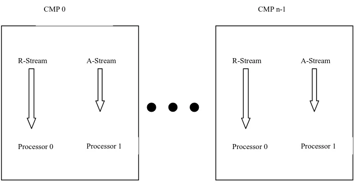
Figure 1-1. Slipstream execution mode for CMP based multiprocessors.

Skipping synchronization routines makes the A-Stream speculative; since we

cannot guarantee that the dependencies enforced by synchronization will be met. A

value produced by the A-Stream cannot be stored to shared memory unless we have

the ability to roll back to its previous value in case of misspeculation. Therefore the

A-Stream processor discards stores to the shared memory. R-Stream correctness is not

affected since the speculative value produced by the A-Stream is never transmitted to

the R-Stream, as local changes to the shared variable are never stored or made visible

to other tasks. Though the A-Stream can bring erroneous data into the shared L2

cache prematurely, this will not affect the R-Stream’s correctness, as the R-Stream

correctly observes the synchronization before consuming data. Data that was

prefetched too early will be invalidated by the producer before the R-Stream tries to

read it.

R-Stream A-Stream

CMP 0 CMP n-1

Processor 0 Processor 1

R-Stream A-Stream

The system-provided synchronization routines are modified in order for the

A-Stream to skip the synchronization points. The R-A-Stream executes the synchronization

routines normally.

1.2 AR-Synchronization

Synchronization between the A-Stream and R-Stream is called

AR-Synchronization. A session is defined as a sequence of instructions that end in a

barrier or an event wait [3][2]. AR-Synchronization is important as it controls the

number of sessions that the A-Stream can be ahead of the R-Stream. A single

counting semaphore [1] is used between each A-Stream–R-Stream pair. The R-Stream

increments the counting semaphore whenever it reaches a barrier. The A-Stream

decrements the counter when it reaches the barrier as long as the counting semaphore

value is not negative. If the counting semaphore value is negative then A-Stream

waits for R-Stream to catch up.

The place where the R-Stream increments the counter determines whether the

type of synchronization is local or global [4]. If the R-Stream increments the counter

as it enters a barrier, then the synchronization observed is called local, as the

corresponding A-Stream observes synchronization only with this R-Stream. In other

words, the A-Stream may proceed, even if other R-Streams have not yet reached the

barrier. If the R-Stream increments the counter as it leaves a barrier, then the

synchronization observed is called global as the corresponding A-Stream observes

1.3 Need for AR-Synchronization

AR-Synchronization mechanism is classified by

1. Number of tokens

2. Type of synchronization: local or global.

The different types of AR-Synchronization for slipstream mode in this study

include one-token local (L1), token local (L0), one-token global (G1) and

zero-token global (G0) [4], [3][2]. One-zero-token local allows the A-Stream to be at most one

session ahead when R-Stream enters the previous synchronization event. Zero-token

local ensures that the A-Stream is in the same session as the R-Stream when R-Stream

enters a synchronization event. One-token global allows the A-Stream to be at most

one session ahead when the R-Stream exits the previous synchronization event.

Zero-token global ensures that the A-Stream is in the same session as the R-Stream when

the R-Stream exits the same synchronization event.

Zero-token global is the tightest synchronization model as the A-Stream has to

be in the same session as the R-Stream when the R-Stream exits the same

synchronization event. One-token local is the loosest, as the A-Stream can enter the

next session when its R-Stream enters the previous synchronization event.

Figure 1-2 shows that for different benchmarks there is no single consistent

winner. For OCEAN, choosing L0 gives the best execution time (winner). For SOR,

L1 is the overall winner, and L0 is the winner for MG benchmark though there is little

difference among all four methods. OCEAN and MG benchmark were chosen for

0 20 40 60 80 100 120 140

SOR OCEAN MG Benchmark

E x e c u ti o n t im e i n m il li o n s L0 L1 G0 G1

Figure 1-2. Execution time for the four synchronization methods for 8CMP.

To obtain the best execution time for a particular benchmark, all four

synchronization methods should be executed by specifying the method at runtime. A

program might benefit if we vary the synchronization mode between different regions

of code. To incorporate such dynamic synchronization, the synchronization method

should be able to be varied at every session. This result in a speedup when compared

to the best execution time obtained from executing the four methods on an individual

basis. But such aggressive switching might incur some overhead. Sliding-window

method overcomes this problem by maintaining a particular method for a number of

sessions before changing it to another synchronization method.

1.4 Contributions and Organization of Thesis

1.4.1

1. We show that choosing dynamic synchronization will usually provide a speedup

when compared to choosing a particular AR-Synchronization method during

program execution.

2. We implement a method to check whether there is any benefit in dynamically

varying synchronization methods in between each barrier for an application. The

criterion to consider, in order to dynamically alter the method, is the inter-barrier

execution time. By using the method which provides the minimum time at each

session, we improve the overall execution time. The overall execution time

obtained by switching is compared to the minimum execution time from executing

the four synchronization methods for a particular benchmark. To minimize the

overhead that is incurred due to this aggressive switching, a better algorithm

(sliding-window) is implemented.

3. We implement a mechanism that changes the number of tokens dynamically.

4. We characterize the behavior of various benchmarks with the varying

AR-Synchronization methods.

1.4.2 Organization:

The organization of this thesis is as follows. Chapter 2 gives an overview of

the framework. The design and implementation are described in detail. The

sliding-window method is explained in detail along with results in Chapter 3. In Chapter 4,

Chapter 2

The Framework: Design and Implementation

This chapter describes the implementation of the dynamic

AR-Synchronization mechanism. The Simulation environment and benchmarks are

described in section 2.1. The method used to dynamically vary AR-Synchronization

method at each session is explained in detail in section 2.2. The results are discussed

in section 2.3.

2.1 Experimental Setup

2.1.1 Simulation Environment

A CMP-based multiprocessor is simulated where each node consists of a

dual-processor CMP. Each dual-processor has its own L1 instruction and data cache, whereas

there is only one L2 cache shared between the two processors. The system is

simulated using SimOS [7][8] with IRIX 5.3 and MIPSY CPU model.

Table 2-1. System specifications.

CPU

MIPSY-based CMP model ; Clock Speed:1 GHz

L1 cache L2 cache (unified)

Size: 32KB Size: 1MB

2.1.2Benchmarks

OCEAN, MG and SOR benchmarks were used in this study. OCEAN is taken

from Splash-2 [11]. MG is an OPENMP port of NAS Parallel Benchmark 2.3[5].

1. OCEAN [9][11]: This application studies the role of eddies and boundary

currents in influencing large-scale ocean movements. The application uses

finite differencing CFD with a regular grid. The algorithm uses red-black

Gauss-Seidel multi-grid equation solver; each time-step of the simulation

involves setting up and solving a set of partial differential equations.

2. MG [5]: This benchmark uses a V-cycle MultiGrid method to compute the

solution of the 3-D scalar Poisson equation.

3. SOR: This solves partial differential equation on a grid where each interior

element is computed using its value and the value of its four neighbors.

The grid points are alternately assigned as red and black points.

The input data sizes are shown in Table 2-2.

Table 2-2. Benchmarks grid size.

Application Grid Size

Ocean 258×258, 128×128, 66×66

SOR 1024×1024

2.2 Methodology

This thesis tries to address three issues:

1. Is there a benefit if the AR-Synchronization is varied during program

execution?

2. If there is a benefit, can the adaptive scheme be implemented?

3. How should the dynamic scheme be implemented?

2.2.1 Basis for switching

AR-Synchronization can be varied based on different criteria. We chose

inter-barrier execution time as our basis for varying the synchronization. Inter-inter-barrier

execution time is the time between two synchronization points or is the session time.

By trying to minimize this session time we can minimize the overall execution time

thus providing a speedup. We ignore barrier time as its contribution is insignificant

compared to the total execution time.

2.2.2

For any benchmark, inter-barrier execution time is obtained by executing the

program with each AR-Synchronization method. Across each session the best time is

chosen and a critical path with the best maximum execution time across all processors

is formed. This critical path with the best maximum execution time forms the trace.

To perform adaptive synchronization, the trace is read in at the time of execution and

The dynamic variation of the methods was limited to varying between L1-L0

and G0-G1. Alternating between global and local methods is beyond the scope of this

thesis and is left for future work.

To show that there is a benefit from toggling between synchronization

methods, projected execution time is calculated from the critical path. By adding the

synchronization time obtained from the method with the best execution time to the

critical path we obtain the projected execution time. This analysis assumes that we

want to vary between L0 and L1 only.

For SOR there was a 2.9% decrease in execution time. This is shown in Table

2-3 and Figure 2-1. MG has 0.02% decrease in execution time. OCEAN has a 0.4%

increase in execution time when compared to the best execution time.

Table 2-3. Projected Execution Time for various benchmarks.

Benchmark

Winner (Method with best execution

time)

Winner’s Execution time (Million cycles)

Projected Execution time (Million cycles)

SOR L1 37.8 36.6

MG L0 35.9 35.9

Projected Execution Time

SOR OCEAN MG

Benchmark % d e c re a s e i n e x e c u ti o n t im e

Figure 2-1. Projected execution time for various benchmarks.

2.2.3 Implementation of adaptive algorithm

A counting semaphore is present between each A-Stream, R-Stream pair.

Upon reaching a barrier, the A-Stream decrements the counter and can proceed as

long as the counter is not negative. The R-Stream increments the counting semaphore

before entering a barrier (local) or while leaving the barrier (global).

To implement the adaptive scheme we use the pre-generated trace file to

determine which AR-Synchronization method should be used for that session. The

values from the trace are read in at every session. The counting semaphore was

incremented originally, by calling the routine to increment the counting semaphore at

every session. This was done by the R-Stream. The algorithm is modified to prevent

the R-Stream from incrementing the semaphore (to decrease the number of tokens), or

to increment by more than one (to increase the number of tokens). For example, if L1

trace, the counting semaphore is not incremented by the R-Stream for the second

session, as the A-Stream would already be ahead and would have reached the next

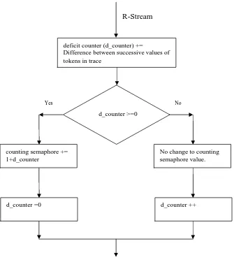
session. The algorithm is shown in Figure 2-2.

We introduce a deficit counter, which is the difference in token count between

two consecutive sessions from the trace. We increment the semaphore counter only if

the deficit counter is positive. The semaphore counter is incremented by the deficit

counter value, if the deficit counter is positive. The deficit counter keeps track of the

token changes in the trace and thus limits the A-stream movement according to the

trace. For example, in the trace if L0 is to be used for a session, then the deficit

counter value will be 0−0 = 0, assuming that the synchronization mechanism in the

previous session is also L0. Now since the value is zero, the semaphore counter is

incremented by one. Suppose for the next session, the synchronization method to be

used is L1. Now the deficit counter value is 1−0=1. The semaphore counter is

incremented by 2 allowing the A-Stream to be ahead by a session. This algorithm was

implemented and the results were compared with the projected execution time as well

Figure 2-2. Flowchart describing the algorithm used to change synchronization method.

2.3 Results

The actual execution time obtained from varying the AR Synchronization

method based on the trace read in during program execution is presented in Table 2-4. d_counter >=0

counting semaphore += 1+d_counter

deficit counter (d_counter) +=

Difference between successive values of tokens in trace

R-Stream

No change to counting semaphore value.

d_counter =0 d_counter ++

Table 2-4. Actual execution time obtained for various benchmarks by varying the synchronization method. Benchmark Winner (Method with best execution time) Winner’s Execution time (Million cycles) Projected Execution time (Million cycles) Actual Execution time (Million cycles)

SOR L1 37.8 36.6 33.9

MG L0 35.9 35.9 35.9

OCEAN L0 109.4 109.9 120.5

There was a 10% decrease in the total execution time for SOR benchmark.

OCEAN performed the worst with 10% increase in the total execution time. There

was not a big difference in MG with a change of 0.09%. This is shown in Figure 2-3.

-15.00% -10.00% -5.00% 0.00% 5.00% 10.00% 15.00%

SOR OCEAN MG

benchmark % d e c re a s e i n e x e c t im e

Figure 2-3. Decrease in execution time after implementing dynamic synchronization.

The reason for OCEAN’s poor performance is the frequent switching of the

method is only 8. That is, a method is used at the maximum for 2% of the total

number of sessions before changing to the other synchronization mechanism. This

increased the overall inter-barrier time compared to the one obtained from the trace.

MG showed the expected performance as the overall execution time of all the

synchronization methods were close to each other as shown in Figure 1-2. There was

infrequent switching in SOR.

Though it is shown that the dynamic switching of AR-Synchronization method

did result in speedup, such frequent switching resulted in some overhead such as

increased inter-barrier time. In the next chapter, we introduce a method to reduce the

Chapter 3

Sliding-window method

3.1

When AR-Synchronization varies for every session, there is some overhead

which we believe impairs the speedup that could have been obtained otherwise. The

total benefit due to this adaptive synchronization method is hampered by such

aggressive switching. For example in the trace, if L1 is the best method to be used in

the first session, followed by L0 in the next session, followed by L1, then it is more

advantageous to change the L0 to L1. This is because the A-Stream would already be

ahead. This can be done only if the time contributed by L1 was less than that of L0.

To analyze this, we incorporated a sort of sliding-window method to decide when to

vary the AR-Synchronization method.

We already know the result of picking the best synchronization method for the

entire run of a program. In the trace we try to change to the alternate synchronization

mechanism after using the best synchronization method for a certain number of

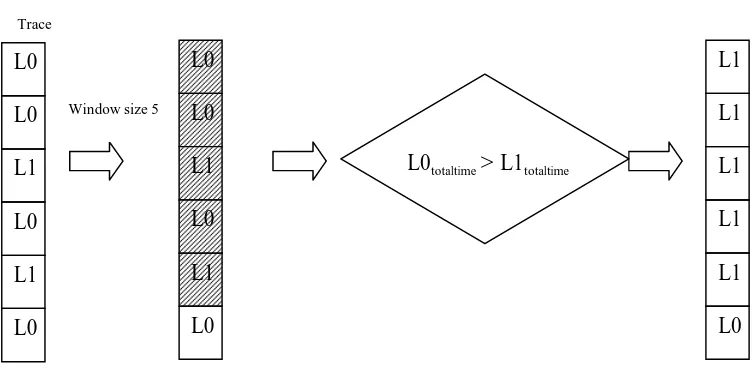
sessions. In this experiment we vary between L0 and L1 only. For any window size N,

we slide through the trace for that specific window size. If we find the time occupied

by the alternate method is less for a particular window, then we change every session

in that window to the alternate method. By doing this we don’t frequently change the

size of 5. We change every method in that window range to L1, as the time consumed

by L1 is less than the time occupied by L0. However in Figure 3-2, the total time for

L0 is less than L1 and we don’t change everything to L0. This is because we are

aware of the result if we use a single method (in this case L0) for the entire run. We

only want to change to the other method (L1) for all the sessions in the window if the

total time taken by L0 is greater than the total time taken by L1.

Figure 3-1. Sliding-window method for window size of 5.

This method allows the benefit of retaining one method for certain number of

sessions before switching to another AR-Synchronization method. If we wait for

several sessions before changing the method, we improve the overall execution time

as we don’t frequently switch methods. This is similar to starting out with only the

winner synchronization method and changing the method whenever the alternate

method’s execution time is less than the winner for that session. The modified trace is

then used in the program execution.

L0 L0 L1 L1 L0 L0 L0 L0 L1 L1 L0 L0 L1 L1 L1 L1 L1 L0

Window size 5 Trace

Figure 3-2. Sliding-window method.

3.2

Various window sizes were applied to the trace obtained for different

benchmarks and the results were analyzed.

3.2.1 OCEAN

OCEAN has 363 sessions. The window size was varied by 10. As mentioned

in Section 3.1, for any given window size, we slide through the trace and change the

synchronization method to the method with total minimum time for that window size.

The results are shown in Figure 3-3.

L0

L0

L1

L1 L0

L0

L0

L0

L1

L1 L0

L0

L1

L1

L1

L1 L1

L0

Window size 5 Trace

No change to trace

-2.00% -1.00% 0.00% 1.00% 2.00% 3.00% 4.00% 5.00% 6.00% 7.00%

10 20 30 40 50

Window size % d e c re a s e i n e x e c u ti o n t im e execution time

Figure 3-3. Ocean window size vs. execution time.

For a window size of 30, there is a decrease of more than 6% in the total

execution time. Retaining the original trace would have resulted in a 10% increase in

the execution time. Figure 3-4 (a) shows that majority of the sessions were occupied

by L0 (67%) which had the best overall execution time. The percentage of total

inter-barrier time occupied by this 67% (L0) is nearly 82%, as shown in Figure 3-5 (a). By

applying a window size of 30, we show in Figure 3-4 (b) that nearly 50% of the

sessions are occupied by L1. The percentage of the total inter-barrier time occupied

by the method did not change as shown in Figure 3-5 (b). This just means that we

eliminated the frequent switching while maintaining the time occupied by a particular

Figure 3-4. (a) Original trace (b) Modified trace by applying sliding-window method, Ocean: Number of sessions occupied by a method.

Figure 3-5. (a) Original trace (b) Modified trace by applying sliding-window method, Ocean: Percentage of Inter-barrier time occupied by a method.

33.05%

66.90%

L1 L0

49.50%

50.41% L1

L0

17.81%

82.18%

L1 L0

18.18%

81.81%

3.2.2 SOR -0.50% 0.00% 0.50% 1.00% 1.50% 2.00% 2.50% 3.00% 3.50%

3 6 9 12 15 18

Window size % d e c re a s e i n e x e c u ti o n t im

e execution time

Figure 3-6. SOR window size vs. execution time.

There are only 20 barriers present in SOR. We vary the window size by 3. We

can see that for window size of 15, there was more than 3% decrease in the total

execution time. If we had retained the original trace then we would have obtained a

10% decrease in the execution time. The original trace had only one instance of L1

and can be considered as the result of choosing a window size of one. Figure 3-7 (a)

shows that majority of the sessions (90%) used L0, which had the best overall

execution time. The percentage of total inter-barrier time occupied by this 90% (L0) is

nearly 92% as shown in Figure 3-7 (b)Figure 3-8. By applying a window size of 15,

we show in Figure 3-8 (a) that nearly 80% of the sessions use L1. The percentage of

as shown in Figure 3-8 (b). SOR executes the piece of code for red-black

implementation repeatedly. Therefore the change in the number of sessions occupied

by a method should reflect in the time occupied by the sessions in the critical path.

Figure 3-7. (a) Original trace (b) Modified trace, SOR: Number of sessions occupied by a method.

Figure 3-8. (a) Original trace (b) Modified trace, SOR: percentage of inter-barrier time occupied by a method

95.00% 5.00%

L0 L1

20.00%

80.00%

L0 L1

91.94% 8.05%

L0 L1

20.49%

79.59%

3.2.3 MG -1.00% -0.80% -0.60% -0.40% -0.20% 0.00% 0.20% 0.40%

10 20 30 40 50 60

Window size % d e c re a s e i n e x e c u ti o n t im e execution time

Figure 3-9. MG window size vs. execution time

We vary the window size for MG by 10. We can see that for window size of

40, there was nearly 0.2% decrease in the total execution time. If we had retained the

original trace then we would have obtained a 0.09% decrease in the execution time.

Figure 3-10 (a) shows that majority of the sessions used L0 (59%), which had the best

overall execution time. The percentage of the total inter-barrier time occupied by this

59% (L0) is only 5% as shown in Figure 3-10 (b). We show in Figure 3-11(a) that by

applying a window size of 40, nearly 10% of the sessions are occupied by L1. The

percentages of the total inter-barrier time occupied by this L0 method did not vary

much as shown in Figure 3-11 (b). This is because for MG, as shown in Figure 1-2,

the execution time for all four synchronization methods are close to one another, and

Figure 3-10. (a) Original trace (b) Modified trace, MG: Number of sessions occupied by a method.

Figure 3-11. (a) Original trace (b) Modified trace, MG: percentage of inter-barrier time occupied by a method.

59.92% 40.07%

L0 L1

10.99%

89%

L0 L1

5.70%

94.25%

L0 L1

3.42%

96.58%

3.3 OCEAN: further study

To understand why a particular window size works best, we varied the grid

size for OCEAN benchmark. We used grid sizes of 130×130 and 66×66 in addition to

the grid size 258×258 that we started out with.

For a grid size of 130×130 and a window size of 30, as shown in Figure 3-12,

there was a 7.6 % decrease in execution time.

-6% -4% -2% 0% 2% 4% 6% 8% 10%

10 20 30

window size

%

d

e

c

re

a

s

e

e

x

e

c

u

ti

o

n

t

im

e

Figure 3-12. OCEAN with grid size 130×130.

For a grid size of 66×66 we see that for a window size of 40 we obtain the

A window size in the range of 30-40 works best for OCEAN. If the window

size is very large then only one method will dominate the trace. Sliding-window size

for a grid size of 258×258 saturates at 60, i.e., only one method occupies the trace;

there is no switching to the other method for a window size of 60. We find that using

window size of 30 gives the maximum speedup. Similarly for a grid size of 66×66,

window size saturates at 60, but the maximum speedup can be obtained at a window

size of 30. Though it is not clear why a particular window size works best, we find

that a window size which lies in the middle range works best.

-3% -2% -1% 0% 1% 2% 3%

10

20

30

40

50

60

70

window size % d e c re a s e i n e x e c u ti o n t im e execution time

Figure 3-13. OCEAN with grid size 66×66.

We wanted to verify that there is no big variation in the result if we use a

window size close to the one which gave us the best speedup. For a grid size of

258×258, when we vary the window size in the range of 26-34, we get the following

0 1 2 3 4 5 6 7 8 9

26 27 28 29_{Window size}30 31 32 33 34

% d e c re a s e i n e x e c u ti o n t im e execution time

Figure 3-14. OCEAN grid size 258×258.

Figure 3-14 shows that there is a 7.9% decrease in the execution time for a

window size of 28. Sensitivity around the best window size in general does not vary

Chapter 4

Related Work

This thesis work is closely related to that of Ibrahim [4]. The key aspect of the

initial work is preserved in this thesis. However new technique has been developed

that is unique to this thesis. Varying synchronization method at runtime, at every

session, in an application is not explored in the previous work. One of the four

synchronization methods must be specified at run time. It is not possible to know

which of the four synchronization methods will emerge as the winner with minimum

execution time. Trying out all the four methods is time consuming. It would be better

if we could change the methods dynamically.

In this thesis, the possibility of such an adaptive scheme is analyzed and

experiments are performed on various benchmarks to explore the feasibility of such

switching of synchronization methods. With the help of a pre-defined trace we have

shown that it is possible to vary synchronization methods while executing an

application.

A similar work, the reactive synchronization algorithm [6], chooses among

shared-memory and message-passing protocols in response to the level of contention.

Reactive spin locks combines the low latency of a test-and-set lock with the

scalability of Mellor-Crummey and Scott (MCS) queue locks, and dynamically

chooses between them. A method based on consensus objects for efficiently selecting

but the lock itself. When invalid consensus is reached, the process will retry the

synchronization operation with another protocol. The consensus object allows the

process to decide whether it is executing the right protocol. The performance of the

reactive algorithm is close to the best of any of the passive algorithms at all levels of

contention. However this method fails when contention levels vary too frequently.

Similar to this method we try to dynamically vary synchronization methods

based on the pre-defined trace. The Pre-formed trace contains the best maximum

Chapter 5

Summary and Future Work

5.1 Summary

This research investigated whether varying slipstream methods dynamically

will provide a speedup when compared to fixing a particular AR-Synchronization

method throughout program execution. For most of the benchmarks we looked at,

there was a considerable decrease in the execution time, thus providing a speedup.

MG was the only exception, but analysis showed that there was no room for

improvement as all the four synchronization methods yielded execution time close to

one another.

We also derived a method to check whether it is possible to achieve benefit by

dynamically varying synchronization methods in between each barrier present for an

application. The criterion to consider in order to dynamically vary is the inter-barrier

execution time. By using the method which provided the minimum critical path time

at each session, we improve the overall execution time. The overall execution time

obtained by switching is compared to the minimum execution time from executing the

four synchronization methods for a particular benchmark. Using the sliding-window

algorithm on the trace yielded a 7.9% decrease in the execution time for OCEAN and

5.2 Future Work

We are interested in varying the synchronization method according to the

nature of the program. The synchronization method will vary with different

applications; therefore it is necessary to understand the application before suggesting

a method to be used for that application.

We also want to implement the actual varying of the scheme adaptively at

runtime. This could be based on a particular parameter of that program. We could also

run the application with all the methods for a particular number of iterations and

decide the best method, and use it for the rest of the application if the program is of

iterative nature.

One of our future goals is also to alternate between local and global

Bibliography

[1] E.W Dijkstra, Cooperating sequential processes, Academic Press, 1968

[2] K.Z Ibrahim, and G.T Byrd, “Extending OpenMP to Support Slipstream

Execution Mode,” Proceeding of the 17th International Parallel and Distributed

Processing Symposium, April 2003.

[3] K.Z Ibrahim, G.T Byrd, and E. Rotenberg, Slipstream Execution Mode for

CMP-Based Multiprocessors. 9th Int'l Conf. on High-Performance Computer

Architecture, Feb. 2003.

[4] K.Z Ibrahim, Slipstream Execution Mode for CMP-Based shared memory systems

(Dissertation), 2003.

[5] H. Jin, M. Frumkin, and J. Yan, The OpenMP Implementations of NAS Parallel

Benchmarks and Its Performance. TR NAS-99-011, NASA Ames Research

Center, October 1999.

[6] B.H Lim, and A. Agarwal, Reactive Synchronization Algorithms for

Multiprocessors. In Sixth International Conference on Architectural Support for

Programning Languages and Operating Systems (ASPLOS VI), pp. 25-35, 1994.

[7] M. Rosenblum, S. A. Herrod, E. Witchel, and A. Gupta. Complete computer

system simulation: the simos approach. IEEE Parallel and Distributed

Technology: Systems and Applications, 3(4):34--43, Winter 1995.

[8] http://stanford.simos.edu

[9] J. P. Singh and J. L. Hennessy. Finding and exploiting parallelism in an ocean

simulation program: Experiences, results, implications. Journal of Parallel and

[10] K. Sundaramoorthy, Z. Purser, and E. Rotenberg, Slipstream processors:

Improving both Performance and Fault Tolerance. In Architectural Support for

Programming Languages and Operating Systems, pp. 257-268, 2000.

[11] S. Woo, M. Ohara, E. Torrie, J.P Singh, and A. Gupta, The SPLASH-2

Programs: Characterization and Methodological Considerations. 22nd Int'l Symp.