Implementation and Validation of the Viscoelastic Continuum Damage Theory for Asphalt Mixture and Pavement Analysis in Brazil

ABSTRACT

NASCIMENTO, LUIS ALBERTO HERRMANN DO. Implementation and Validation of the Viscoelastic Continuum Damage Theory for Asphalt Mixture and Pavement Analysis in Brazil. (Under the direction of Dr. Y. Richard Kim).

This dissertation presents the implementation and validation of the viscoelastic continuum damage (VECD) model for asphalt mixture and pavement analysis in Brazil. It proposes a simulated damage-to-fatigue cracked area transfer function for the layered viscoelastic continuum damage (LVECD) program framework and defines the model framework’s fatigue cracking prediction error for asphalt pavement reliability-based design solutions in Brazil.

The research is divided into three main steps: (i) implementation of the simplified viscoelastic continuum damage (S-VECD) model in Brazil (Petrobras) for asphalt mixture characterization, (ii) validation of the LVECD model approach for pavement analysis based on field performance observations, and defining a local simulated damage-to-cracked area transfer function for the Fundao Project’s pavement test sections in Rio de Janeiro, RJ, and (iii) validation of the Fundao project local transfer function to be used throughout Brazil for asphalt pavement fatigue cracking predictions, based on field performance observations of the National MEPDG Project’s pavement test sections, thereby validating the proposed framework’s prediction capability.

For the first step, the S-VECD test protocol, which uses controlled-on-specimen strain mode-of-loading, was successfully implemented at the Petrobras and used to

accurate for fatigue life predictions of Brazilian asphalt mixtures, even when very different asphalt binders are used. Also, the applicability of the load amplitude sweep (LAS) test for the fatigue characterization of the asphalt binders was checked, and the effects of different asphalt binders on the fatigue damage properties of the asphalt mixtures was investigated. The LAS test results, modeled according to VECD theory, presented a strong correlation with the asphalt mixtures’ fatigue performance.

In the second step, the S-VECD test protocol was used to characterize the asphalt mixtures used in the 27 selected Fundao project test sections and subjected to real traffic loading. Thus, the asphalt mixture properties, pavement structure data, traffic loading, and climate were input into the LVECD program for pavement fatigue cracking performance simulations. The simulation results showed good agreement with the field-observed

distresses. Then, a damage shift approach, based on the initial simulated damage growth rate, was introduced in order to obtain a unique relationship between the LVECD-simulated shifted damage and the pavement-observed fatigue cracked areas. This correlation was fitted to a power form function and defined as the averaged reduced damage-to-cracked area transfer function.

presented good agreement, following the same trends found for the Fundao project pavement sites.

Implementation and Validation of the Viscoelastic Continuum Damage Theory for Asphalt Mixture and Pavement Analysis in Brazil

by

Luis Alberto Herrmann do Nascimento

A dissertation submitted to the Graduate Faculty of North Carolina State University

in partial fulfillment of the requirements for the Degree of

Doctor of Philosophy

Civil Engineering

Raleigh, North Carolina 2015

APPROVED BY:

_______________________________ ______________________________

Dr. Y. Richard Kim Dr. Akhtarhusein Tayebali

Committee Chair

DEDICATION

BIOGRAPHY

Luis Alberto Herrmann do Nascimento was born the younger of two sons to Luiz and Vera Nascimento on September 27, 1977. Born in Oriximiná, PA, in Brazil’s North region, he grew up in Rio Grande do Sul state in Brazil’s South region. During the summer of 1995 Luis Alberto enrolled at the Federal University of Rio Grande do Sul to pursue a degree in Civil Engineering and graduated in December of 1999 with a concentration in Geotechnical Engineering. From 1999 to 2003 he worked as a Civil Engineer in Cientec’s Geothecnical Department in the city of Porto Alegre, RS. Next, Luis Alberto moved to Rio de Janeiro, RJ, to work as a researcher in asphalt binder and asphalt pavement materials and design at Petrobras. In 2006 he enrolled at the Federal University of Rio de Janeiro to pursue a Master of Science degree in Civil Engineering, which he obtained in December of 2008. In the intervening years Luis Alberto has progressed to a Consultant position at Petrobras, and then, during the fall of 2011, while still working at Petrobras, he enrolled at North Carolina State University in Raleigh, NC to pursue his Ph.D. degree in Civil Engineering. Luis Alberto

ACKNOWLEDGMENTS

First of all, I would like to acknowledge my gratitude to Petrobras for funding my studies at North Carolina State University and for all the support this company has given me throughout my research. A special thank-you goes to my amazing coworker (now retired) and great mentor, Dr. Leni Leite, for her guidance in my research experience. I would also like to thank the Petrobras’ managers, Vania Periquito and Maria Helena Ramos, for their support and confidence in my work. I want to thank all the Petrobras and BR Distributor asphalt team colleagues. A special thanks to Sergio Rocha, Ulisses Figueiredo, Marcos Chacur, and Marcos Fritzen. I could not have completed this work without their help.

Also, I would like to acknowledge the research team members of the universities associated with the Brazilian National MEPDG project for their collaboration on a tremendous amount of field work and data collection that were very important for

accomplishing this research study. A special thanks to professors Dr. Laura Motta and Dr. Jorge Soares for their helpful advice and comments during my research.

I would like to thank my advisory committee members for agreeing to serve and also for their assistance and guidance. I offer very special thanks to my brilliant advisor, Dr. Y.Richard Kim, for his guidance and support throughout my student life at NC State.

I feel very grateful to have been able to work with my current and former NC State colleagues. I would also to acknowledge the friendship from Shayan Safavizadeh,

TABLE OF CONTENTS

LIST OF TABLES………..…iv

LIST OF FIGURES………..viii

CHAPTER 1. INTRODUCTION ... 1

1.1. BACKGROUND ... 1

1.2. OBJECTIVES ... 3

CHAPTER 2. THEORETICAL BACKGROUND ... 4

2.1. VISCOELASTIC CONTIL ... 4

2.1.1. VECD Theory ... nuum Damage (VECD) Mode7 2.1.2. Simplified Viscoelastic Continuum Damage (S-VECD) Model ... 24

2.1.3. Failure Criteria ... 35

2.2. PAVEMENT PERFORMANCE ANALYSIS USING THE VECD MODEL ... 46

2.2.1. The VECD-FEP++ Program ... 49

2.2.2. Layered Viscoelastic Continuum Damage (LVECD) Analysis Program ... 70

CHAPTER 3. BRAZILIAN PAVEMENT SITES USED IN THE

RESEARCH ...83

3.1. OVERVIEW ... 83

3.2. FUNDAO PROJECT PAVEMENT SITES ... 85

3.2.2. Traffic ... 93

3.2.3. Climate ... 94

3.2.4. Pavement Test Sections ... 98

3.2.5. Pavement Test Section Condition Surveys ... 103

3.3. NATIONAL MEPDG PROJECT PAVEMENT SITES ... 109

3.3.1. Pavement Test Sections ... 111

3.3.2. Traffic ... 115

3.3.3. Climate ... 117

3.3.4. Pavement Test Section Condition Surveys ... 121

CHAPTER 4. MATERIALS AND TEST METHODS FOR ASPHALT

MIXTURE CHARACTERIZATION ...123

4.1. MATERIALS ... 123

4.1.1. S-VECD Model Implementation Study Asphalt Mixtures ... 124

4.1.2. Fundao Project Asphalt Mixtures ... 127

4.1.3. National MEPDG Project Asphalt Mixtures ... 131

4.2. TEST METHODS ... 136

4.2.1. Linear Viscoelastic (LVE) Characterization Methodology ... 136

4.2.4. Test Specimen Fabrication ... 147

CHAPTER 5. RESULTS AND ANALYSIS ...150

5.1. S-VECD MODEL IMPLEMENTATION STUDY ... 150

5.1.1. LVE Characterization ... 150

5.1.2. S-VECD Model Fatigue Characterization ... 156

5.1.3. S-VECD Model Fatigue Test Simulations... 164

5.1.4. Effect of Binder Type on Asphalt Mixture Fatigue Performance ... 175

5.2. FUNDAO PROJECT PAVEMENT SIMULATIONS ... 182

5.2.1. Asphalt Mixture Characterization ... 182

5.2.2. Fundao Project Test Sections: Fatigue Damage Simulations ... 194

5.2.3. Defining Damage-to-Cracked Area Transfer Functions ... 205

5.3. NATIONAL MEPDG PROJECT PAVEMENT SIMULATIONS ... 231

5.3.1. Asphalt Mixture Characterization ... 231

5.3.2. National MEPDG Project Test Sections: Fatigue Damage Simulations... 243

5.3.3. Validating the Damage-to-Cracked Area Transfer Functions ... 256

5.4. FATIGUE CRACKING PREDICTION RELIABILITY ... 267

5.5. PROPOSED LVECD MODEL PROTOCOL APPLICATION FOR ASPHALT PAVEMENT DESIGN IN BRAZIL ... 271

LIST OF TABLES

Table 1. Pavement properties and loading used in simulations by Kim et al. (2009) ... 53

Table 2. VECD-FEP++ simulation results showing the aging effect in Florida and Wyoming pavements (Baek et al. 2012) ... 65

Table 3. Homogeneous pavement segment locations and layer thicknesses ... 90

Table 4. Pavement classification criteria for IRI and GGI (Pinto and Preussler 2002) ... 92

Table 5. Asphalt mixtures used in the Fundao project... 102

Table 6. Fundao project test sections considered in this study ... 102

Table 7. ‘Percent cracked area’ of the Fundao project test sections ... 108

Table 8. National MEPDG project pavement test sections ... 111

Table 9. Asphalt mixtures used in the National MEPDG project test sections ... 112

Table 10. National test section traffic levels for the first in-service year and date of traffic opening ... 115

Table 11. ‘Percent cracked area’ of the National MEPDG project test sections ... 122

Table 12. Gradation distribution of the S-VECD model implementation study asphalt mixtures... 125

Table 13. Binders chosen for the S-VECD implementation study asphalt mixtures ... 126

Table 14. Gradation distribution of the Fundao project asphalt mixtures ... 128

Table 15. Binders used in the Fundao project asphalt mixtures ... 130

Table 16. Fundao project test section asphalt mixtures ... 131

Table 17. Gradation distribution for the National MEPDG project asphalt mixtures ... 133

Table 19. Asphalt mixtures used in the National MEPDG project ... 136 Table 20. Implementation study asphalt mixtures: mastercurves and shift factor function fitting coefficients ... 151 Table 21. Implementation study asphalt mixtures: relaxation modulus Prony representation fitting coefficients (a) ... 154 Table 22. Implementation study asphalt mixtures: relaxation modulus Prony representation fitting coefficients (b) ... 155 Table 23. Implementation study asphalt mixtures: damage ratio exponents () ... 156 Table 24. Fatigue testing data for PPA, RA-TB, and HIMA mixtures ... 157 Table 25. Implementation study asphalt mixtures: average damage characteristic curves and GR failure envelope regression coefficients ... 162 Table 26. FAFs and af values at 19°C ... 180

Table 27. Implementation study asphalt mixtures: rankings determined from FAFM, FAFB,

and af , controlled-strain ... 181

Table 32. Fundao project asphalt mixtures: averaged damage characteristic curves and GR failure envelope regression coefficients ... 189 Table 33. Fundao project test sections chosen for initial pavement analysis ... 195 Table 34. Initial test sections: traffic level, number of ESALs (USACE) ... 195 Table 35. Averaged reduced damage-to-cracked area transfer function final fitting

LIST OF FIGURES

Figure 1. Stress-strain behavior for controlled-stress cyclic loading within the material´s LVE range ... 10 Figure 2. Stress-pseudo strain behavior for controlled-stress cyclic loading within the

material´s LVE range ... 11 Figure 3. Typical input and responses for: a) controlled-stress (CS) uniaxial cyclic test (input vs. time), b) CS (stress vs. pseudo strain), c) controlled-crosshead (CX) uniaxial cyclic test (input vs. time), and d) CX (stress vs. pseudo strain) (Underwood et al. 2009a) ... 15 Figure 4. Example of change in pseudo stiffness (C) versus number of cycles in a typical controlled-strain uniaxial cyclic damage-inducing test at 20°C (Nascimento 2014) ... 17 Figure 5. Damage parameter (S) versus number of cycles for on-specimen controlled-strain uniaxial cyclic damage testing with different inputs (Nascimento 2014) ... 21 Figure 6. Pseudo stiffness (C) versus number of cycles for on-specimen controlled-strain uniaxial cyclic damage testing with different inputs (Nascimento 2014) ... 21 Figure 7. Pseudo stiffness (C) versus damage parameter (S) characteristic curves for on-specimen controlled-strain uniaxial cyclic damage testing with different inputs (Nascimento 2014) ... 22 Figure 8. Schematic view of the stress, pseudo strain, and pseudo stiffness definitions used in the simplified and rigorous modeling approaches (Underwood et al. 2009a) ... 26 Figure 9. Schematic of effect of M factor on dC/dt used in the simplified calculations

Figure 11. Experimental observation of pseudo stiffness values at failure versus reduced frequency (Hou 2009) ... 37 Figure 12. RDEC versus number of cycles during controlled-crosshead uniaxial cyclic loading (Zhang 2012) ... 39 Figure 13. Schematic representation of total released pseudo strain energy in stress-pseudo strain space (Zhang et al. 2013) ... 42 Figure 14. (a) History of R

C

W in the controlled-crosshead test and (b) rate of R C

W in the

controlled-crosshead test (Zhang et al. 2013) ... 42 Figure 15. R

G0 versus Nf results for different modes of loading (Sabouri and Kim 2014) .... 43

Figure 16. GR versus Nf results for different modes of loading (Sabouri and Kim 2014) .... 45

Figure 36. Maximum deflections in the central lane, determined during the initial survey

using the Benkelman beam ... 89

Figure 37. Homogeneous pavement segments: thicknesses of the layers ... 91

Figure 38. Pavement condition classification based on IRI and GGI values... 92

Figure 39. Fundao project pavement sites: hourly traffic distribution... 93

Figure 40. Daily average low and high temperatures for Rio de Janeiro International Airport (Weather Spark 2014) ... 95

Figure 41. Fractions of days in which various types of precipitation are observed for Rio de Janeiro International Airport (Weather Spark 2014) ... 96

Figure 42. Average daily minimum, maximum, and average wind speeds for Rio de Janeiro International Airport (Weather Spark 2014) ... 97

Figure 43. Overlay techniques used for pavement rehabilitation in the Fundao project ... 99

Figure 44. Fundao project asphalt overlay over a partially milled asphalt surface ... 99

Figure 45. Fundao project full milling pre-overlay example: image of the granular base just before its recompaction ... 100

Figure 46. Fundao project partial milling plus SAM pre-overlay surface example ... 100

Figure 47. Distress allocation scheme ... 104

Figure 48. Average maximum deflections of all test sections ... 107

Figure 49. Average maximum deflections of each test section ... 107

Figure 50. National MEPDG project test section pavement structures ... 114

Figure 53. Daily average low and high temperatures for Porto Alegre, RS (Weather Spark 2014) ... 117 Figure 54. Daily average low and high temperatures for Ribeirao Preto, SP (Weather Spark 2014) ... 119 Figure 55. Daily average low and high temperatures for Criciuma, RS (Weather Spark 2014) ... 120 Figure 56. Gradation distribution chart for the S-VECD model implementation study asphalt mixtures... 125 Figure 57. Gradation distribution chart for the 19.1 mm NMAS Fundao project asphalt mixtures... 128 Figure 58. Gradation distribution chart for the 12.5 mm NMAS Fundao project asphalt mixtures... 129 Figure 59. Gradation distribution chart for the 9.5 mm NMAS Fundao project asphalt

Figure 65. Tensile on-specimen strain-only input (400 ) and steady-state load output for typical COS uniaxial fatigue test; 10 Hz, from cycle 1900 to 1905 ... 146 Figure 66. MLPC BBMAX 80 French mixer illustration ... 147 Figure 67. (a) S-VECD fatigue test specimen, (b) end plates and gluing jig, and (c) specimen ready for fatigue testing ... 149 Figure 68. Implementation study asphalt mixture mastercurves in semi-log scale, TR = 20°C

... 152 Figure 69. Implementation study asphalt mixture mastercurves in log-log scale, TR = 20°C

... 152 Figure 70. Implementation study asphalt mixture phase angles, TR = 20°C ... 153

Figure 71. PPA asphalt mixture damage characteristic curves, TR = 20°C ... 158

Figure 72. RA-TB asphalt mixture damage characteristic curves, TR = 20°C ... 158

Figure 73. RA-TB asphalt mixture average damage characteristic curves, TR = 20°C ... 159

Figure 74. HIMA asphalt mixture damage characteristic curves, TR = 20°C ... 159

Figure 75. PPA asphalt mixture: GR versus Nf failure envelope, TR = 20°C ... 160

Figure 76. RA-TB asphalt mixture: GR versus Nf failure envelope, TR = 20°C ... 161

Figure 77. HIMA asphalt mixture: GR versus Nf failure envelope, TR = 20°C ... 161

Figure 78. Implementation study asphalt mixtures: average damage characteristic curves, TR

= 20°C ... 163 Figure 79. Implementation study asphalt mixtures: GR versus Nf failure envelopes, TR = 20°C

Figure 80. Comparison between experimental and predicted on-specimen strains versus Nf

for the PPA, RA-TB, and HIMA asphalt mixtures ... 165 Figure 81. Comparison between experimental and predicted on-specimen strains for the PPA, RA-TB, and HIMA asphalt mixtures ... 166 Figure 82. Implementation study asphalt mixtures: fatigue life simulations at 15°C and 10 Hz ... 167 Figure 83. Implementation study asphalt mixtures: fatigue life simulations at 20°C and 10 Hz ... 167 Figure 84. Implementation study asphalt mixtures: fatigue life simulations at 25°C and 10 Hz ... 168 Figure 85. 50/70 mixture fatigue life simulations at 10 Hz and different temperatures ... 170 Figure 86. 30/45 mixture fatigue life simulations at 10 Hz and different temperatures ... 170 Figure 87. 15/25 mixture fatigue life simulations at 10 Hz and different temperatures ... 171 Figure 88. E´´ at 10 Hz versus temperature for the 50/70, 30/45, and 15/25 asphalt mixtures ... 171 Figure 89. E´ at 10 Hz versus temperature for the 50/70, 30/45, and 15/25 asphalt mixtures ... 172 Figure 90. Nfat 300  and 10 Hz at different temperatures for the 50/70, 30/45, and 15/25

Figure 93. Implementation study asphalt binders: fatigue envelopes at 19°C ... 177 Figure 94. Implementation study asphalt binders: crack length at failure (af) at 19°C ... 178

Figure 95. Fatigue area factor (FAF) graphical representation... 179 Figure 96. Comparison of FAFs and af values at 19°C ... 180

Figure 97. Fundao project asphalt mixtures: mastercurves in semi-log scale, TR = 20°C (a)

... 183 Figure 98. Fundao project asphalt mixtures: mastercurves in semi-log scale, TR = 20°C (b)

... 184 Figure 99. Fundao project asphalt mixtures: mastercurves in log-log scale, TR = 20°C (a) 184

Figure 100. Fundao project asphalt mixtures: mastercurves in log-log scale, TR = 20°C (b)

... 185 Figure 101. Fundao project asphalt mixtures: phase angles, TR = 20°C (a) ... 185

Figure 102. Fundao project asphalt mixtures: phase angles, TR = 20°C (b) ... 186

Figure 103. Fundao project asphalt mixtures: averaged damage characteristic curves, TR =

20°C (a) ... 190 Figure 104. Fundao project asphalt mixtures: averaged damage characteristic curves, TR =

20°C (b) ... 190 Figure 105. Fundao project asphalt mixtures: GR versus Nf failure envelopes, TR = 20°C (a)

... 191 Figure 106. Fundao project asphalt mixtures: GR versus Nf failure envelopes, TR = 20°C (b)

Figure 107. Fundao project asphalt mixtures: fatigue life simulations at 20°C and 10 Hz (a) ... 192 Figure 108. Fundao project asphalt mixtures: fatigue life simulations at 20°C and 10 Hz (b) ... 193 Figure 109. Initial Fundao test sections: fatigue ‘percent cracked area’ evolution ... 195 Figure 110. Initial Fundao test sections: average deflection basins (FWD) ... 197 Figure 111. Grid of 110 points considered in the average damage calculation (N/Nf) ... 200

Figure 112. Averaged damage versus time data simulated in the LVECD program: Fundao project initial test sections ... 201 Figure 113. TS 19: damage contour at 60 months, N/Nf ... 202

Figure 114. TS 34: damage contour at 60 months, N/Nf ... 202

Figure 115. TS 37: damage contours at 6 and 60 months, N/Nf ... 202

Figure 116. TS 40: damage contours at 60 months, N/Nf ... 203

Figure 117. Damage color scale ... 203 Figure 118. Core sample obtained from TS 19, where top-down cracking can be observed 204 Figure 119. Fundao project initial test sections: cracked area versus averaged damage in arithmetic scale ... 205 Figure 120. Fundao project initial test sections: cracked area versus averaged damage in semi-log scale... 206 Figure 121. Scheme of T0.35 and R12-1 calculations ... 207

Figure 123. Fundao project initial test sections: averaged damage level at 10% of cracked area versus R12-1 ... 209

Figure 124. Fundao project initial test sections: cracked area versus averaged damage curve-fitting in semi-log scale ... 210 Figure 125. Fundao project test sections: (a) averaged damage versus time simulated in the LVECD program (a) ... 211 Figure 126. Fundao project test sections: (b) averaged damage versus time simulated in the LVECD program (b) ... 211 Figure 127. Test section symbols used for the data presented in Figure 125 and Figure 126 (and elsewhere in this dissertiation) ... 212 Figure 128. All Fundao project test sections: cracked area versus averaged damage in

arithmetic scale ... 213 Figure 129. All Fundao project test sections: cracked area versus averaged damage in semi-log scale ... 214 Figure 130. All fatigue-cracked Fundao project test sections: averaged damage level at 10% cracked area versus T0.35 ... 214

Figure 131. All fatigue-cracked Fundao project test sections: averaged damage level at 10% cracked area versus R12-1 ... 215

Figure 132. All fatigue-cracked Fundao project test sections: additive shift factor (Δ) versus T0.35 – reference reduced damage of 0.5 for 10% cracked area ... 217

Figure 134. All fatigue-cracked Fundao project test sections: multiplicative shift factor (S) versus T0.35 – reference reduced damage of 0.5 for 10% cracked area ... 218

Figure 135. All fatigue-cracked Fundao project test sections: multiplicative shift factor (S) versus R12-1 – reference reduced damage of 0.5 for 10% cracked area ... 218

Figure 136. All Fundao project test sections: cracked area versus averaged reduced damage based on

35 . 0

T

S in semi-log scale ... 220

Figure 137. All Fundao project test sections: cracked area versus averaged reduced damage based on

1 12

R

S in semi-log scale ... 221

Figure 138. AASHTO MEPDG bottom-up fatigue cracking sigmoidal transfer function: United States national calibration (NCHRP 2004) ... 222 Figure 139. Averaged reduced damage-to-cracked area transfer function curve-fitting based on

35 . 0

T

S in semi-log scale ... 224

Figure 140. Averaged reduced damage-to-cracked area transfer function curve-fitting based on

1 12

R

S in semi-log scale ... 224

Figure 141. Comparison of observed versus predicted cracked areas based on

35 . 0

T

S ... 225

Figure 142. Comparison of observed versus predicted cracked areas based on

1 12

R

S ... 226

Figure 143. Comparison of observed versus predicted cracked areas of four Fundao project test sections, based on

35 . 0

T

S ... 228

Figure 144. Observed and predicted (

35 . 0

T

S ) cracked areas versus ESALs: TS 34 ... 229

Figure 145. Observed and predicted (

35 . 0

T

Figure 146. Observed and predicted (

35 . 0

T

S ) cracked areas versus ESALs: TS 58 ... 230

Figure 147. Observed and predicted (

35 . 0

T

S ) cracked areas versus ESALs: TS 89 ... 230

Figure 148. National project asphalt mixtures: mastercurves in semi-log scale, TR = 20°C (a)

... 233 Figure 149. National project asphalt mixtures: mastercurves in semi-log scale, TR = 20°C (b)

... 233 Figure 150. National project asphalt mixtures: mastercurves in log-log scale, TR = 20°C (a)

... 234 Figure 151. National project asphalt mixtures: mastercurves in log-log scale, TR = 20°C (b)

... 234 Figure 152. National project asphalt mixtures: phase angles, TR = 20°C (a) ... 235

Figure 153. National project asphalt mixtures: phase angles, TR = 20°C (b) ... 235

Figure 154. National project asphalt mixtures: averaged damage characteristic curves, TR =

20°C (a) ... 239 Figure 155. National project asphalt mixtures: averaged damage characteristic curves, ... 239 Figure 156. National project asphalt mixtures: GR versus Nf failure envelopes, TR = 20°C (a)

... 240 Figure 157. National project asphalt mixtures: GR versus Nf failure envelopes, TR = 20°C (b)

Figure 159. National project asphalt mixtures: fatigue life simulations at 20°C and 10 Hz (b) ... 241 Figure 160. National MEPDG project test sections: averaged damage versus time simulated using LVECD program (a)... 245 Figure 161. National MEPDG project test sections: averaged damage versus time simulated using LVECD program (b) ... 245 Figure 162. UFSM 1: damage contours at 12 and 36 months, N/Nf ... 246

Figure 163. UFSM 3: damage contours at 12 and 36 months, N/Nf ... 246

Figure 164. UFRGS 2: damage contours at 12 and 36 months, N/Nf ... 247

Figure 165. USP 4: damage contours at 12 and 36 months, N/Nf ... 247

Figure 166. USP 5: damage contours at 12 and 36 months, N/Nf ... 248

Figure 167. UFSC 2: damage contours at 12 and 36 months, N/Nf ... 248

Figure 168. UFSC 3: damage contours at 12 and 36 months, N/Nf ... 249

Figure 169. ND 1: damage contours at 12 and 36 months, N/Nf ... 249

Figure 170. ND 2: damage contours at 12 and 36 months, N/Nf ... 250

Figure 171. ND 3: damage contours at 12 and 36 months, N/Nf ... 250

Figure 172. ND 4: damage contours at 12 and 36 months, N/Nf ... 251

Figure 173. ND 5: damage contours at 12 and 36 months, N/Nf ... 251

Figure 174. ND 6: damage contours at 12 and 36 months, N/Nf ... 252

Figure 175. ND 7: damage contours at 12 and 36 months, N/Nf ... 252

Figure 176. ND 8: damage contours at 12 and 36 months, N/Nf ... 253

Figure 178. ND 10: damage contours at 12 and 36 months, N/Nf ... 254

Figure 179. Damage color scale ... 254 Figure 180. National MEPDG project test sections: cracked area versus averaged reduced damage based on

35 . 0

T

S ... 257

Figure 181. National MEPDG project test sections: cracked area versus averaged reduced damage based on

1 12

R

S ... 257

Figure 182. Fundao and National MEPDG test sections: cracked area versus averaged reduced damage based on

35 . 0

T

S ... 259

Figure 183. National MEPDG project test sections: comparison of observed versus predicted cracked areas based on

35 . 0

T

S ... 259

Figure 184. National MEPDG project test sections: comparison of observed versus predicted cracked areas based on

1 12

R

S ... 260

Figure 185. Fundao and National MEPDG test sections: comparison of observed versus predicted cracked areas based on

35 . 0

T

S ... 261

Figure 186. Fundao and National MEPDG test sections: comparison of observed versus predicted cracked areas based on

1 12

R

S ... 261

Figure 187. National MEPDG project test sections: comparison between observed and predicted cracked areas (

35 . 0

T

S ) determined from last field survey ... 263

Figure 188. National MEPDG project test sections: comparison between Nobserved and Npredicted

(

35 . 0

T

Figure 189. Prediction error versus average reduced damage (

35 . 0

T

S ): all test sections ... 268

Figure 190. Standard error of the mean versus averaged reduced damage (

35 . 0

T

S ): all test

CHAPTER 1.

INTRODUCTION

1.1.

BACKGROUND

Fatigue cracking is the major distress in asphalt concrete pavements in Brazil. This phenomenon has a complex nature that is related to both the material and structural

characteristics of asphalt concrete pavements. Currently in Brazil, the available tests and analysis protocols are not reliable for the accurate prediction of the fatigue performance of asphalt mixtures and pavements. Many Brazilian researchers have proposed different test methods and specimen geometries for fatigue damage characterization, such as the bending beam, indirect tension, trapezoidal tests, etc. Typically, the results of these tests, at a single temperature, are fitted to power law fatigue curves (Wöhler curves) and used with simplified pavement layered elastic analysis for performance prediction. In this regard, different

empirical approaches have been taken by Brazilian pavement engineers, but without any validation or carefully defined laboratory-to-field transfer functions.

A fatigue performance model that can be used effectively in pavement design and preservation must have two main components: (i) a fatigue damage growth relationship that describes how damage grows as a function of loading frequency, temperature, and load level, and (ii) a failure criterion that can be used to define the fatigue life of asphalt concrete

(Sabouri and Kim 2014). Thus, to properly understand and model fatigue cracking over the range of conditions encountered in the field without performing a large number of

repeated loading, particularly the process of cracking (Underwood et al. 2009a). In addition, these mechanistic models should be incorporated into a pavement analysis framework, which in turn should be validated for engineering applications through extensive comparisons between predicted and field-observed performance, in order to develop a proper simulated damage-to-cracked area transfer function and to determine the analysis framework’s prediction capability.

Viscoelastic continuum damage (VECD) theory has been used successfully for asphalt mixture characterization in the United States. This mechanistic approach makes use of fundamental material properties to characterize the behavior of asphalt concrete

effectively under a wide range of conditions using an efficient, simplified laboratory test program. The key feature of the VECD model is the damage characteristic curve, which is a material property that is independent of test conditions. This property, with proper

implementation into the pavement analysis framework, can be used to predict the fatigue damage of asphalt layers over the range of conditions encountered in the field (Kim 2009).

Researchers at North Carolina State University have implemented the VECD model into a layered VECD analysis framework, referred to as the layered viscoelastic continuum damage (LVECD) program (Eslaminia et al. 2012). This tool has shown potential to be used

countries (Park 2013), but so far, no transfer function has been defined for using this tool for asphalt pavement fatigue cracking predictions.

1.2.

OBJECTIVES

The objectives of this research project are:

 to implement the VECD model for the characterization of Brazilian asphalt mixtures and validate the modeling approach for mixtures composed of a wide range of asphalt binders;

 to check the applicability of the load amplitude sweep (LAS) test for the fatigue characterization of asphalt binders and investigate the effects of different asphalt binders on the linear viscoelastic (LVE) and fatigue damage properties of asphalt mixtures;

 to simulate the fatigue performance of Brazilian asphalt pavement test sections under real traffic loading using the analysis framework that is based on the VECD model (i.e., the LVECD program); and

CHAPTER 2.

THEORETICAL BACKGROUND

The main goal of this chapter is to present the theories and concepts found in the literature that are needed for this research effort. Because one of the research goals is the implementation of the VECD model in Brazil, including pavement analyses and field validation, the main topics of the literature review are:

 the theoretical background of the VECD and S-VECD models and

 pavement performance analysis and experiences using the LVECD program.

2.1.

VISCOELASTIC CONTINUUM DAMAGE (VECD) MODEL

According to Hou et al. (2010), various laboratory testing methods and models have been developed to assess the fatigue performance of HMA. One of the most popular testing methods is the flexural bending test, also known as the beam fatigue test, which measures the fatigue life of a compacted asphalt beam subjected to repeated flexural bending. The standard procedure for the beam fatigue test is described in the AASHTO T-321 standard, and was adopted by researchers at the University of California Berkeley under the Strategic Highway Research Program (SHRP) Project A-003A (Tangella et al. 1990; Tayebali et al. 1995). Other techniques also have been proposed, such as trapezoidal fatigue testing (EN 12697-24; Rowe 1993), direct tension testing (Raithby and Sterling 1972), and indirect tension testing (Roque and Buttlar 1992; Buttlar and Roque 1994; Nascimento et al. 2010).

In addition to the different testing protocols, analysis methods also differ. The

relationship wherein the effects of strain or stress level and material properties (the modulus, for example) on cycles to failure are modeled (Hou et al. 2010). This is the basic model form used in the National Cooperative Highway Research Program (NCHRP) 1-37A Mechanistic-Empirical Pavement Design Guide (MEPDG). However, other researchers have analyzed test results using energy-based methods (Carpenter and Shen 2006; Shen and Carpenter 2007), fracture mechanics (Majidzadeh et al. 1971; Salam 1971; Monistmith and Salam 1973), thermomechanical damage concepts (Lundstrom et al. 1994; Bodin et al. 2004a), and continuum damage mechanics (Bodin et al. 2004b; Bazant and Pjaudier-Cabot 1989; Kim and Little 1990; Lee and Kim 1998a; Lee and Kim 1998b, Daniel and Kim 2002; Hou et al. 2010; Babadopulos 2014; Nascimento et al. 2014).

The continuum damage mechanics-based model was used in the work presented in this dissertation. The VECD model makes use of fundamental material properties to characterize the behavior of asphalt concrete effectively using an efficient, simplified

laboratory test program. This approach is particularly useful because, although VECD theory itself is somewhat complicated, it is amenable to simplifying assumptions that only slightly reduce the predictive capabilities, but greatly improve the model’s usability (Hou et al. 2010).

(Lee and Kim 1998a; Lee and Kim 1998b). Subsequent work by Daniel and Kim showed that the damage characteristics of asphalt concrete are material properties and can be determined using a simplified procedure, such as the constant crosshead rate monotonic direct tension test (Daniel and Kim 2002). Chehab et al. showed that the time-temperature superposition (t-TS) principle can be extended from a material’s LVE range to high damage levels, which helps reduce the required testing time significantly (Chehab et al. 2002; Chehab et al. 2003). In work by Underwood et al., these principles were applied to mixtures tested at the Federal Highway Administration Accelerated Load Facility (FHWA ALF) in McLean, VA, and the applicability of VECD modeling principles to both modified and unmodified asphalt concrete mixtures was demonstrated. Also, the fatigue resistance ranking of the ALF mixtures using the VECD model was successfully predicted (Underwood et al. 2006; Underwood et al. 2009b).

The VECD model that is based on the constant crosshead rate monotonic test has some practical shortcomings. One is that the model characterization requires constant

crosshead rate testing, and the peak load level necessary to perform such a test is close to the load capacity of the Asphalt Material Performance Tester (AMPT). Thus, it is important to have a model that not only is applicable for cyclic fatigue test data, but also can be

Kutay et al. applied a simplified form of the VECD model to both controlled-stress and controlled-crosshead (CX) push-pull tests (Kutay et al. 2008). However, these modeling approaches all have limited applications due to certain faults in the rigor of the theoretical application. Underwood et al. proposed a more rigorously accurate simplified model that has been able to correct the deficiencies in the other models (Underwood et al. 2009a;

Underwood et al. 2009b; Underwood et al. 2009c).

The most recent work has been done by Sabouri and Kim (2014) who used the VECD model for asphalt mixture characterization and proposed a fatigue failure criterion based on the rate of release of the pseudo strain energy (GR), which is independent of the mode-of-loading and temperature. This failure criterion requires characterization tests at only a single temperature and a single mode-of-loading, thereby significantly reducing the costs associated with testing.

2.1.1.VECD Theory

principles. In Schapery’s theory, damage is quantified by an internal state variable (S) that accounts for microstructural changes in the material. Other researchers have utilized elastic-based nonlocal continuum damage theories for this purpose (Bazant and Pijaudier-Cabot 1989; Bodin et al. 2004), whereas still others have assumed that the internal state variables are related directly to the strain history, both viscoelastic and viscoplastic, of the material (Levenburg and Uzan 2004; Uzan and Levenburg 2007).

The VECD model is built on three main concepts: (i) the elastic-viscoelastic correspondence principle based on pseudo strain (εR

) for modeling the viscoelastic behavior of the material, (ii) the continuum damage mechanics-based work potential theory for modeling the effects of microcracks on global constitutive behavior, and (iii) the t-TS

principle with growing damage to include the combined effects of time/rate and temperature. In order to explain VECD theory more fully, these concepts are described in the next

sections.

2.1.1.1.Elastic-Viscoelastic Correspondence Principle

The stress-strain relationships for many viscoelastic materials can be represented by elastic-like equations through the use of so-called pseudo variables. This simplifying feature enables a class of extended correspondence principles to be established and applied to linear as well as some nonlinear analyses of viscoelastic deformation and fracture behavior

(Schapery 1984). Using these correspondence principles, one can obtain viscoelastic

The usual Laplace transform-based correspondence principle is limited to LVE behavior with time-varying boundary conditions, whereas the correspondence principles that are based on pseudo variables are applicable to both the linear and nonlinear behavior of a class of viscoelastic materials with stationary or time-dependent boundary conditions. Also, the correspondence principles do not require a transform inversion step to obtain the

viscoelastic solutions but rather requires a convolution integral that is much easier to handle than the inversion step. Consider a stress-strain equation for LVE materials,

(1) where

σ and ε = stress and strain tensors,

E(t) = the relaxation modulus matrix, ξ = reduced time, and

τ = the integration variable.

Equation (1) can be written as:

(2) if εR

is defined as

(3) where ER is the reference modulus, which is a constant and has the same dimensions as the

relaxation modulus. The usefulness of Equation (2) is that a correspondence can be found







0 _d d

with the linear elastic stress-strain relationship. That is, Equation (2) takes the form of elastic stress-strain equations even though they are actually viscoelastic stress-strain equations. The pseudo strain is referred to as εR

. If ER is equal to one in Equation (3), the pseudo strain is

simply the LVE stress response to a particular strain input (Kim 2009).

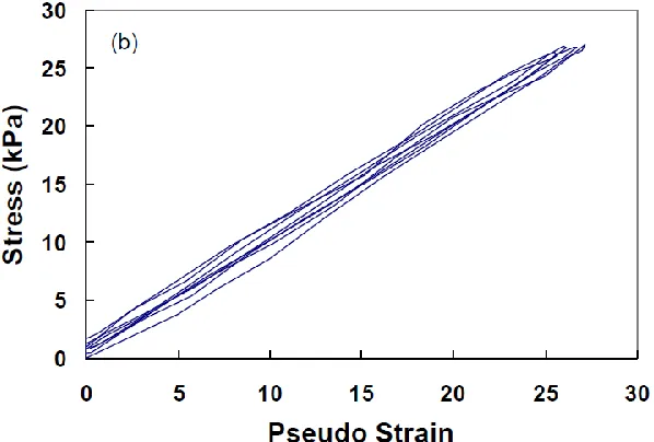
The power of pseudo strain can be seen in Figure 1 and Figure 2. Figure 1 shows the stress-strain behavior for controlled-stress cyclic loading within the material’s LVE range (such as for a complex modulus test). Because the material is being tested in its LVE range, no damage is induced, and the hysteretic behavior and accumulating strain are due to

viscoelasticity only. Figure 2 shows the same stress data plotted against the calculated pseudo strains. All of the cycles collapse to a single line with a slope of 1.0 (ER = 1.0). The use of

pseudo strain essentially accounts for the viscoelasticity of the material and allows for the separate characterization of damage within the specimen.

Figure 2. Stress-pseudo strain behavior for controlled-stress cyclic loading within the material´s LVE range

2.1.1.2.Work Potential Theory

In continuum damage mechanics, the damaged body can be viewed as a

homogeneous continuum on a macroscopic scale, and the effect of the damage typically is reflected in terms of the reduction in stiffness or strength of the material (Kim 2009). The state of damage can be quantified by a set of parameters often referred to as internal state variables or damage parameters in the context of thermodynamics of irreversible processes.

The growth of damage is governed by an appropriate damage evolution law. The stiffness of the material, which varies with the extent of the damage, is determined as a function of the internal state variables by fitting the theoretical model to available experimental data.

isentropic processes). These potentials are point functions of thermodynamic state variables. When thermal effects are not considered, both the Helmholtz free energy and Gibbs free energy potentials are identified as so-called strain energy and represent the energy stored in the system that is algebraically equal to the work done in the system by external loading. However, when damage occurs due to external loading, the work done in the body is not stored entirely as strain energy because part of it is consumed, thereby causing damage to the body. The amount of energy required to produce a given amount of damage is expressed as a function of the internal state variables. The total work that is input to the body during the processes in which damage occurs depends, in general, on the path of loading. However, it has been observed that, for certain processes in which damage occurs, the work input is independent of the path of loading (Schapery 1987; Lamborn and Schapery 1988, 1993).

Based on these concepts, Schapery (1990) developed a theory using the

thermodynamics of irreversible processes to describe the mechanical behavior of elastic composite materials with growing damage. The following three fundamental elements comprise Schapery’s work potential theory.

1)Strain energy density function:

(4) 2)Stress-strain relationship:

(5)





W W  ,

 

3)Damage evolution law:

(6) where σ and ε are the stress and strain tensors, respectively; Sm are the internal state variables;

and Ws = Ws(Sm) is the dissipated energy that is due to structural changes. Using Schapery’s

elastic-viscoelastic correspondence principle and a rate-type damage evolution law (Schapery 1984 and 1990; Park et al. 1996), the physical strain, ε, is replaced with pseudo strain, εR

, to include the effect of viscoelasticity. The use of pseudo strain as defined in Equation (3) accounts for all the hereditary effects of the material through the convolution integral. Thus, the strain energy density function W = W(ε , Sm) transforms to the pseudo strain energy

density function:

(7)

However, the elastic-viscoelastic correspondence principle cannot be used to transform the elastic damage evolution law to use with viscoelastic materials, because both the available force for the growth of Sm and the resistance against the growth of Sm in the

damage evolution law are rate-dependent for most viscoelastic materials (Park et al. 1996). Therefore, the following form, which is similar to power law crack growth laws, is used to describe the damage evolution in a viscoelastic material:

(8) m s m dS dW dS dW  





R R R

S W

W   ,

where S_m is the damage evolution rate, WR is the pseudo strain energy density function, and

m is the material constant. According to Park et al. (1996), the constant m is based on LVE

fracture mechanics. In many viscoelastic crack growth problems, the crack speed is governed by the th _{power in the pseudo energy release rate, in which }

m is related to the material’s

creep or relaxation properties. For example, m = 1+1/n, where n = - logE(t)/log(t) at times,

depending on the crack speed, was shown by Schapery (1975) for rubber.

In the case of asphalt mixture VECD characterization, according to Underwood et al. (2009a), the power, m, is related to the log-log slope of the relaxation modulus, n, and is

dependent upon the type of test used in characterizing the model. For monotonic or CX tests, m = 1/n + 1. For controlled-stress tests in either a push-pull or pull-pull configuration, m =

1/n. It is important to mention that some equations in this dissertation refer to m as simply.

2.1.1.3.Determination of the Damage Parameter (S)

The method that is selected to solve the damage evolution law in Equation (8) is a matter of preference and, as such, two solutions are hereby proposed. The first, proposed by Park et al. (1996), transforms the original equation to an integrated form, and assumes and defines a new parameter, Ŝ. Equation (9) presents, in discrete form, the method proposed by Park et al.

(9) where Ŝ is given by Equation (10):



 1 1

1 1 1

ˆ _ 

  

 

(10)

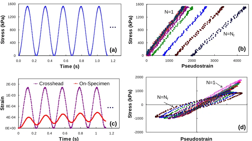
Lee and Kim (1998a, b) also proposed a solution that utilizes the chain rule and makes no assumptions regarding . They conducted uniaxial tensile cyclic loading tests with various load amplitudes to study the mechanical behavior of asphalt concrete. In damage-induced testing, they observed that the slope of the stress–pseudo strain loop decreases as loading continues in both controlled-stress and controlled-strain tests. Figure 3 illustrates the change in the slope of the stress-pseudo strain loop for typical uniaxial cyclic damage-induced testing.

Figure 3. Typical input and responses for: a) controlled-stress (CS) uniaxial cyclic test (input

vs. time), b) CS (stress vs. pseudo strain), c) controlled-crosshead (CX) uniaxial cyclic test (input vs. time), and d) CX (stress vs. pseudo strain) (Underwood et al. 2009a)

0 400 800 1200 1600

0.0 0.2 0.4 0.6 0.8 1.0 1.2

Time (s) Str ess (kPa) 0 400 800 1200 1600

0 1000 2000 3000 4000

Pseudostrain Str ess (kPa) 0E+00 4E-04 8E-04 1E-03 2E-03

0 0.2 0.4 0.6 0.8 1 1.2

Time (s) Str ai n Crosshead On-Specimen -2000 -1000 0 1000 2000 Pseudostrain Str ess (kPa) N=1 N=Nf N=1 N=N_f 0 400 800 1200 1600

0.0 0.2 0.4 0.6 0.8 1.0 1.2

Time (s) Str ess (kPa) 0 400 800 1200 1600

0 1000 2000 3000 4000

Pseudostrain Str ess (kPa) 0E+00 4E-04 8E-04 1E-03 2E-03

0 0.2 0.4 0.6 0.8 1 1.2

Time (s) Str ai n Crosshead On-Specimen -2000 -1000 0 1000 2000 Pseudostrain Str ess (kPa) N=1 N=Nf N=1 N=N_f (a) (c) (b) (d) 0 400 800 1200 1600

0.0 0.2 0.4 0.6 0.8 1.0 1.2

Time (s) Str ess (kPa) 0 400 800 1200 1600

0 1000 2000 3000 4000

Pseudostrain Str ess (kPa) 0E+00 4E-04 8E-04 1E-03 2E-03

0 0.2 0.4 0.6 0.8 1 1.2

Time (s) Str ai n Crosshead On-Specimen -2000 -1000 0 1000 2000 Pseudostrain Str ess (kPa) N=1 N=Nf N=1 N=N_f 0 400 800 1200 1600

0.0 0.2 0.4 0.6 0.8 1.0 1.2

Time (s) Str ess (kPa) 0 400 800 1200 1600

0 1000 2000 3000 4000

Pseudostrain Str ess (kPa) 0E+00 4E-04 8E-04 1E-03 2E-03

0 0.2 0.4 0.6 0.8 1 1.2

Time (s) Str ai n Crosshead On-Specimen -2000 -1000 0 1000 2000 Pseudostrain Str ess (kPa) N=1 N=Nf N=1 N=N_f (a) (c) (b) (d)





 

ˆ _{S C C t}

The change in the slope of the loop represents the reduction in the stiffness of the material as damage accumulates. To represent the change in slope, Lee and Kim (1998b) used the secant pseudo stiffness, SR, defined as:

(11) where R

m

 is the pseudo strain, and σm, which comes from the experimental data, is the stress

that corresponds to R m

 . In modeling, Lee (1996) found it necessary to normalize the pseudo stiffness by the initial pseudo stiffness, I, to account for sample-to-sample variation. The normalized pseudo stiffness, C, is then

(12)

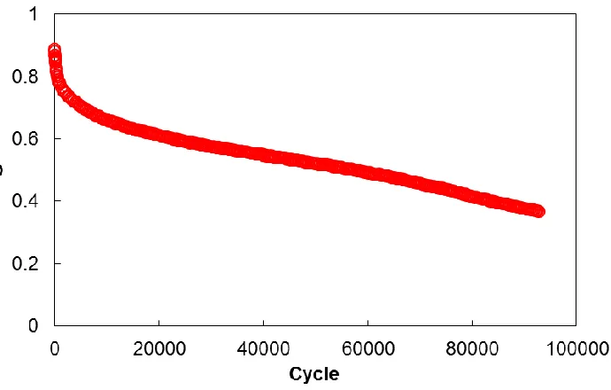
Figure 4 shows typical changes in the C versus number of cycles for a controlled-strain uniaxial cyclic damage-inducing test at 20°C.

R m m R

S   

I S C

R

Figure 4. Example of change in pseudo stiffness (C) versus number of cycles in a typical controlled-strain uniaxial cyclic damage-inducing test at 20°C (Nascimento 2014)

The uniaxial constitutive equations for linear elastic and LVE materials with and without damage are useful to show how the more complex models evolved from the simpler ones, as follows:

Elastic body without damage:

(13)

Elastic body with damage:

(14)

Viscoelastic body without damage:

(15) 

 E_R

 

R R

Viscoelastic body with damage:

(16) where ER is a constant and C(Sm) is a function of the internal state variables (ISV) - Sm that

represent the changing stiffness of the material due to microstructural changes, such as accumulating damage. In Equation (13), ER is the Young’s modulus. A correspondence is

seen between the elastic and viscoelastic constitutive equations; that is, the viscoelastic equations take the same form as the elastic ones, with pseudo strain replacing physical strain, as aforementioned.

It must be observed that for the uniaxial case, the work function (WR) is given by Equation (17):

(17)

The function C1 represents SR, as can be seen from Equations (12) and (18):

(18)

To characterize the function C1 in Equation (18), the damage evolution law (Equation

(8)) and experimental data are used. With the measured stresses and calculated pseudo strains, the C1 values can be determined using Equation (12). To find the dependence of C1

on S1, the values of S1 must be obtained using Equation (8). However, the current form of this

 

S

C 

 

 

 

R m R

S C I

W  

 

S

IC 

equation is not suitable for finding S1, because it requires prior knowledge of the C1(S1)

function through Equation (17).

Lee (1996) used the chain rule in Equation (19) to eliminate S1 from the right-hand

side of the evolution equation and obtain an explicit expression for S1, as shown in Equation

(20).

(19)

(20)

Both functions, C1 and mR, are dependent upon time t, and thus, a numerical approximation can be used with the measured data to obtain S1 as a function of time:

(21)

The relationship between C1 and S1 can then be found by performing regression on

the data. The most common functions used for fitting this relationship are shown in Equations (22) and (23).

(22)

(23) where C10, C11, C12, a, and b are the regression constants.

dS dt dt dC dS dC 

 



 t R

m dt dt dC I S 0 1 2 1 1 2   

 

_

 









i i i i i i R

m C C t t

I t S 1 1 1 1 1 1 2 1 2    

 

 

1 11 10 1 1 C S C C S

C  

 

e S

C 1

1

Daniel and Kim (2002) studied the relationship between the damage parameter (S) and the normalized pseudo stiffness (C) under varying loading conditions. The most

significant finding from their study is that a unique damage characteristic relationship exists between C and S, regardless of loading type (monotonic versus cyclic), loading rate, and stress/strain amplitude. In addition, the application of the t-TS principle with growing damage to the C versus S relationships at varying temperatures yields the same damage characteristic curve in the reduced time scale (Chehab et al. 2002). The only condition that must be met in order to produce the damage characteristic relationship is that the test temperature and load rate combination must be such that only the elastic and viscoelastic behavior prevail with negligible, if any, viscoplasticity.

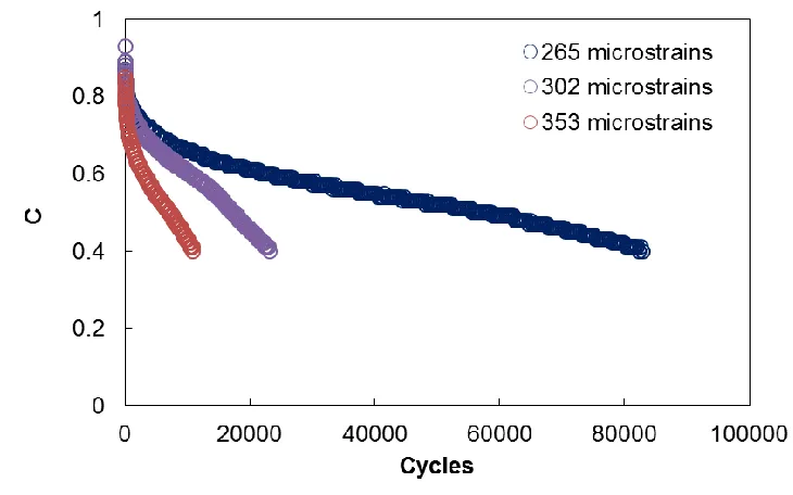
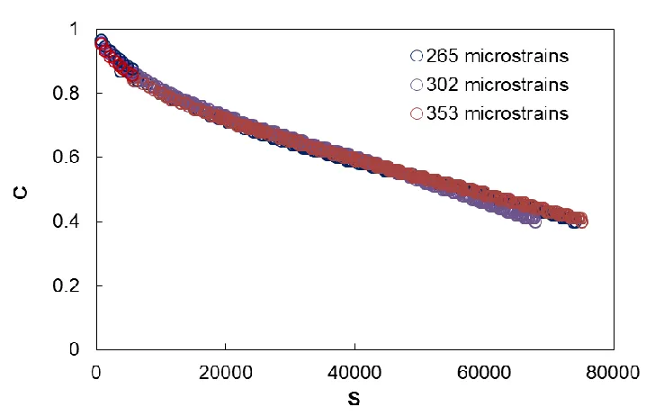
Figure 5 to Figure 7 show the on-specimen controlled-strain uniaxial cyclic damage test results obtained for a styrene-butadiene-styrene (SBS) polymer-modified asphalt

Figure 5. Damage parameter (S) versus number of cycles for on-specimen controlled-strain uniaxial cyclic damage testing with different inputs (Nascimento 2014)

Figure 7. Pseudo stiffness (C) versus damage parameter (S) characteristic curves for on-specimen controlled-strain uniaxial cyclic damage testing with different inputs (Nascimento

2014)

2.1.1.4.Pseudo Strain Calculation: εR

The first step in this characterization process is the calculation of the pseudo strain. In previous work, Equation (3) was solved using a linear piecewise technique, as shown in Equation (24). Such a technique, although fundamentally sound, is profoundly inefficient when analyzing large amounts of data. The source of the inefficiency lies in the need to analyze all the time steps that precede the time step of interest, thus resulting in exponentially increasing the analysis time for the increased data. To overcome this shortcoming, a method commonly used in computational mechanics, the state variable approach, is utilized

(24)

The goal of the state variable approach is to transform the process of convolution into an algebraic operation. Theoretical details of state variable techniques can be found in Simo and Hughes (1998). In a physical sense, though, the state variable approach assigns a variable to each Maxwell element in the Prony representation of the relaxation modulus. This variable then tracks the behavior, or state, of the given element throughout loading (Underwood 2006). The algebraic formulation commonly used for the pseudo strain calculation is shown in Equation (25):

(25)

where η0 and ηi are internal state variables for the elastic response and for the specific

Maxwell element, i, at time step, n+1, respectively. Definitions of these variables are given by Equations (26) and (27), respectively:

(26)

(27) where E, Ei, and ρi are the relaxation modulus fitting coefficients from the Prony

representation, i.e., the elastic modulus, modulus of the ith Maxwell element, and relaxation time, respectively. Equation (25) is a remarkably efficient solution technique for pseudo strain calculation. For comparative purposes, a data set of 4,000 points requires













_

_

_

1 t t

t n t n t n R R d d d t E d d d t E d d d t E

E  

                    



1 1  







1

0  

   



 n

n

E





i t i n i i t n

i e  Ee  

approximately 100 seconds to analyze using Equation (24), but it requires only 1.5 seconds if analyzed by Equation (25) (Underwood 2006).

2.1.2.Simplified Viscoelastic Continuum Damage (S-VECD) Model

According to Underwood et al. (2009a), independent efforts using pseudo strain-based models to obtain the asphalt mixture damage characteristic curve have shown positive results. Christensen and Bonaquist (2005) developed a version of a simplified mechanistic model based on the approach suggested by Kim et al. (2002), whereby simplifications are made in the calculation of the pseudo strain and in the idealization of the input conditions. Christensen and Bonaquist used the continuum damage relationship along with the mixture modulus values and voids filled with asphalt (VFA) to develop a fatigue index for guiding asphalt concrete mixture design. Kutay et al. (2008) applied a form of the VECD model and showed that two different test protocols, controlled-stress and CX push-pull tests, yield the same damage characteristic relationship. Kutay et al. also utilized the damage functions for different FHWA ALF mixtures to predict and rank the mixtures’ field performance.

Although all of these previous research efforts have shown positive results, Underwood et al. (2009a) related that these efforts have certain faults in the rigor of their derivation that limit their application. Thus, Underwood et al. (2009a) reviewed the

application of the continuum damage approach. This model is explained, based on the work done by Underwood et al. (2009a) and Underwood et al. (2012), in the following paragraphs.

The rigorous modeling approach that is based on Equations (3), (12), and (21)

requires that pseudo strain, pseudo stiffness, and damage are calculated for the entire loading history, which is an easy task for the constant crosshead rate test (monotonic test). However, applying this rigorous model to cyclic tests, which can easily have over 10 million data points, is computationally cumbersome, even using modern techniques.

The simplification process proposed by Underwood et al. (2009a) starts with the pseudo strain calculation. Assuming that fatigue damage accumulates only under the tensile loading condition, the pseudo strain tension amplitude, R

ta

, 0

 , is calculated. Instead of using the convolution integral to compute the pseudo strain, a substantial simplification is made by assuming a steady-state condition. In such a condition the pseudo strain can be rigorously computed as the product of the strain and dynamic modulus (at the temperature and frequency commensurate with the test under investigation). This assumption was first proposed by Kim et al. (2003) for analyzing asphalt binder and mastic, but has also been found to introduce only very minor errors when applied to asphalt concrete (Kutay et al. 2008; Underwood et al. 2009a; Underwood et al. 2009b).

2.1.2.1.Pseudo Stiffness Definition for the Simplified Approach

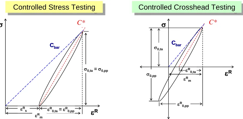
Figure 8 introduces a set of variables used in the simplified formulation for

value (C*). The mathematical definition of each is given in Equations (28) and (29), respectively. The relationship between these two pseudo stiffness values can be found graphically from Figure 8, but is also given in Equation (30).The rigorously defined pseudo stiffness, C, is approximately the same as C*, except that C* is defined as a single quantity for a given cycle, whereas for theoretical rigor C will evolve during a cycle (Underwood et al. 2009a). Note in each equation the presence of the factor, I, which accounts for specimen-to-specimen variability, as aforementioned.

Figure 8. Schematic view of the stress, pseudo strain, and pseudo stiffness definitions used in the simplified and rigorous modeling approaches (Underwood et al. 2009a)

(28)

(29)

Controlled Stress Testing

Controlled Stress Testing Controlled Crosshead Testing_{Controlled Crosshead Testing}

 R C_bar F R m R s C_bar F  R R 0,ta R m R m R 0,pp R

0,ta= R0,pp

0,ta= 0,pp

0,pp

0,ta

Controlled Stress Testing

Controlled Stress Testing Controlled Crosshead Testing_{Controlled Crosshead Testing}

 R C_bar F R m R s C_bar F  R R 0,ta R m R m R 0,pp R

0,ta= R0,pp

0,ta= 0,pp

0,pp

0,ta

C* C*





I C _R s R ta ta R m ta *

* _0,

, 0 , 0        





I

C _R ta _R ta_R

* *

* 0, 0,

(30)

It is important to define the four pseudo strains shown in Figure 8: R

m

 = the absolute pseudo strain at the peak, R

ta

, 0

 = the pseudo strain tension amplitude, R

pp

, 0

 = the peak-to-peak pseudo strain amplitude, and R

s

 = the permanent pseudo strain.

2.1.2.2.Loading Time Associated with Damage Growth in the Simplified Approach

In order to analyze the cyclic data in the simplified mechanics model quickly, it is important to identify the actual time that a given cycle is under tensile loading and also when the damage is growing during this tensile loading. The first attempt at simplification begins with the previous formulation proposed by Daniel and Kim (2002), shown in Equation (31).

(31)

The factor M represents the portion of the pulse during which damage grows. For the particular tests performed by the researchers who developed Equation (31), this portion was approximately one quarter of the total loading pulse time and, thus, M was taken as 4. Noting that the total pulse time is ω/(2π), and using the definition of stress shown in Equation (32), the factor M can be rigorously calculated using Equation (34).

R m R s R m C C







 

2 C M

I

(32)

where ω is the angular frequency and β is a factor that allows direct quantification of the duration that a given stress history is tensile, as obtained from Equation (33).

(33)

Note that when β = 1, the entire stress (and therefore the pseudo strain minus

permanent pseudo strain) history for the given cycle is tensile; when β = 0, half of the history is tensile, and when β = -1, the entire history is compressive. This last condition is not used for any of the tests in this study.

(34)

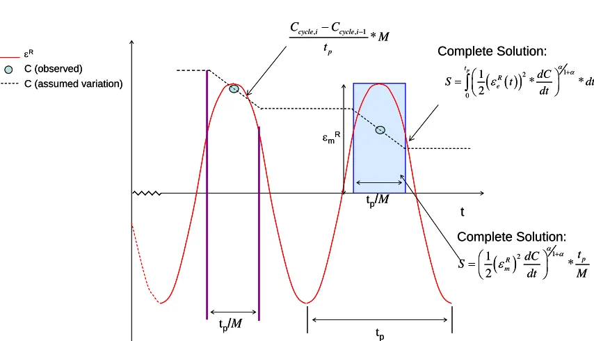
The additional consequence of the factor M is that it implies that pseudo stiffness decreases linearly within a cycle and ignores the fact that the value of the pseudo strain changes throughout the loading cycle. The assumption of linear reduction of the pseudo stiffness is supported through the rigorous mechanical modeling technique (Underwood et al. 2006, Kim and Chehab 2004) and is retained in the simplified analysis protocol. To validate this assumption, damage growth is restricted to conditions under which the stress is between the peak value and half of the peak value (on both the loading and unloading sides). This assumption is shown schematically in Figure 9.

In other words, the time during the loading pulse when the damage growth begins (ξi)

is when half of the ultimate tensile peak value during the loading side is achieved, and the damage growth finishes (ξf) when half of the ultimate tensile peak value during the unloading

side is reached again, as shown in Figure 9. Both times can be determined analytically using Equations (35) and (36).

Figure 9. Schematic of effect of M factor on dC/dt used in the simplified calculations (Underwood et al. 2009a)

(35)

(36)

R

C (observed) C (assumed variation)

t_p

t

t_p/M

, , 1

*

cycle i cycle i p C C M t  

t_p/M

Complete Solution:

 

 ₂ 1 0 1 * * 2 p t R e dC

S t dt

dt  _      _ _ Complete Solution:

 

1 * 2 p R m t dC S dt M        _ _

mR

R

C (observed) C (assumed variation)

t_p

t

t_p/M

, , 1

*

cycle i cycle i p C C M t  

t_p/M

Complete Solution:

 

 ₂ 1 0 1 * * 2 p t R e dC

S t dt

dt  _      _ _ Complete Solution:

 

1 * 2 p R m t dC S dt M        _ _

mR

 

 