A Simple Regression-Based Method to Map Quantitative Trait Loci Underlying Function-Valued Phenotypes

(1)

INVESTIGATION

A Simple Regression-Based Method to Map

Quantitative Trait Loci Underlying

Function-Valued Phenotypes

Il-Youp Kwak,* Candace R. Moore,†_{Edgar P. Spalding,}†_{and Karl W. Broman}‡,1

*Department of Statistics,†Department of Botany, and‡Department of Biostatistics and Medical Informatics, University of Wisconsin, Madison, Wisconsin 53706

ABSTRACT Most statistical methods for quantitative trait loci (QTL) mapping focus on a single phenotype. However, multiple phenotypes are commonly measured, and recent technological advances have greatly simpliﬁed the automated acquisition of numerous phenotypes, including function-valued phenotypes, such as growth measured over time. While methods exist for QTL mapping with function-valued phenotypes, they are generally computationally intensive and focus on single-QTL models. We propose two simple, fast methods that maintain high power and precision and are amenable to extensions with multiple-QTL models using a penalized likelihood approach. After identifying multiple QTL by these approaches, we can view the function-valued QTL effects to provide a deeper understanding of the underlying processes. Our methods have been implemented as a package for R, funqtl.

T

HERE is a long history of work to map genetic loci (quan-titative trait loci, QTL) inﬂuencing quantitative traits. Most statistical methods for QTL mapping, such as interval mapping (Lander and Botstein 1989), focus on a single phenotype. How-ever, multiple phenotypes are commonly measured, and recent technological advances have greatly simpliﬁed the automated acquisition of numerous phenotypes, including phenotypes measured over time. Phenotypes measured over time, an ex-ample of a function-valued trait, have a number of advantages, including the ability to dissect the time course of QTL effects. A simple and intuitive approach to the analysis of such data is to perform QTL analysis at each time point, in-dividually, to identify QTL that affect the phenotype at each time point. This method is simple; however, it does not consider the smooth association across time points, and so it may have less power to detect QTL. Moreover, it can be

difﬁcult to combine the results across time points into a consis-tent story.

A second approach is tofit parametric curves to the data from each individual and treat the parameter estimates as phenotypes in QTL analysis (e.g., see Kendziorskiet al.2002). Maet al.(2002) expanded this approach byfitting a logistic growth model, gðtÞ ¼a=ð1þbe2rt_Þ_; _{at each putative QTL} position, with parameters depending on QTL genotype. This approach can have high power if the model is correct, but it can be difficult to interpret the results if QTL have pleiotropic effects on multiple parameters, and the parameters may have no obvious biologic or mechanistic interpretation.

Another natural approach is to use a nonparametric method so that we do not need to specify the functional shape. For example, Yanget al.(2009) proposed a nonparametric func-tional QTL mapping method that used a certain number of basis functions toﬁt a function-valued phenotype. For example, we might use 10 basis functions. This reduces the dimension from the number of time points to 10, and this is done in a

ﬂexible way, guided by the data. Minet al.(2011) extended this method to multiple-QTL models, using Markov chain Monte Carlo (MCMC) techniques.

Xionget al. (2011) proposed an additional nonparamet-ric functional mapping method based on estimating equa-tions (EE). This method is fast and allows the selection of multiple QTL by a test statistic that they proposed. Sillanpää

Manuscript received May 15, 2014; accepted for publication June 8, 2014; published Early Online June 14, 2014.

Available freely online through the author-supported open access option.

Supporting information is available online athttp://www.genetics.org/lookup/suppl/ doi:10.1534/genetics.114.166306/-/DC1.

1_{Corresponding author: Department of Biostatistics and Medical Informatics, University}

of Wisconsin, 2126 Genetics–Biotechnology Center, 425 Henry Mall, Madison, WI 53706. E-mail: [email protected]

(2)

et al.(2012) proposed another Bayesian multiple-QTL map-ping method based on hierarchical modeling.

Important limitations of existing approaches for the analysis of function-valued traits are that they focus on single-QTL models or exhibit slow speed in multiple-QTL search. We describe two simple methods for QTL mapping with function-valued traits and, following the approach of Broman and Speed (2002) and Manichaikul et al. (2009), extend them for the consideration of multiple-QTL models. We investigate the performance of our approach in computer simulations and apply it to data on a plant growth response known as root gravitropism, which Moore et al.

(2013) measured by automated image analysis over a time course of 8 hr across a population of Arabidopsis thaliana

recombinant inbred lines (RIL). Our aim is to identify the genetic loci (QTL) that inﬂuence the function-valued pheno-type and to characterize their effects over time.

Methods

We focus on the case of RIL. Two inbred strains, say A and B, are crossed and then the F1hybrids are subjected to either selﬁng or sibling mating for many generations to create a new inbred line whose genome is a mosaic of the A and B genomes. This is done multiple times in parallel. At any genomic position, the RIL are homozygous AA or BB.

Single-QTL analysis

The most popular method for QTL mapping is interval mapping, developed by Lander and Botstein (1989). Con-sider a single phenotype, y, and assume there is one QTL, with the modely=m+bq +e, whereqdenotes the QTL genotype, taking the value 0 for genotype AA and 1 for genotype BB, ande N(0,s2_{). Thus}_m_{is the average} phe-notype for QTL gephe-notype AA andbis the effect of the QTL. A key problem is that genotypes are observed only at markers, and we wish to consider positions between markers as putative QTL locations. However, we may calculate p = Pr(q = BB | marker data). The phenotype, given the marker data, then follows a mixture of normal distributions with known mixing proportion,p. An EM algo-rithm (Dempsteret al. 1977) may be used to derive maxi-mum-likelihood estimates of the three parameters,m,b, and s. This is done at each putative QTL location, l. Alterna-tively, one may use regression of y onp to provide a fast approximation (Haley and Knott 1992).

Lander and Botstein (1989) summarized the evidence for a QTL at position l by the LOD score, LOD(l), which is the log10likelihood ratio comparing the hypothesis of a single QTL at position lto the null hypothesis of no QTL. LOD scores in-dicate evidence of presence of QTL. To assess the statistical signiﬁcance of the results, one must deal with the multiple-hypothesis testing issue, from the scan across the genome. This is best handled by a permutation test (Churchill and Doerge 1994). With a function-valued trait, y(t), the model becomes

y(t) =m(t) +b(t)q+e(t). (We focus on the case of a

phe-notype measured over time, but the approach may be ap-plied to any function-valued trait of a single parameter, such as a dose-response curve, or really to any multivariate trait.) The simplest approach is to apply single-QTL analysis for each timet, individually. This gives LOD(t,l) for timetat QTL positionl. We seek to integrate the information across time points to give overall evidence for QTL. Two simple rules are to take the average or maximum LOD scores across times, respectively,

SLODðlÞ ¼1

T

XT

t¼1

LODðt;lÞ

MLODðlÞ ¼max

t LODðt;lÞ;

whereTis the number of time points.

With MLOD, one asks whether there is any time point at which a locus has an effect, while SLOD concerns the overall effect of the locus. MLOD will be more powerful for identifying QTL with large effects over a brief interval of time, while SLOD will be more powerful for identifying loci with effects over a large interval.

To assess signiﬁcance, we permute the rows in the pheno-type matrix relative to rows in the genopheno-type matrix, calculate the statistic across the genome, and record the maximum. We take the 95th percentile of the genome-wide maxima as a 5% signiﬁcance threshold.

Rapid computations are enabled by the simultaneous analysis of the multiple time points. Whereas coefﬁcient estimates at a single time point would be obtained as ^

b¼ ðX9 XÞ21X9 y;with multiple time points we may replace the vectorywith a matrixY, whose columns correspond to the multiple time points. This gives b^¼ ðX9 XÞ21X9Y: The matrix inversion is performed once at each putative QTL position, and the simultaneous analysis of multiple time points is obtained by matrix multiplication, and so the com-putations are linear in the number of time points.

Multiple-QTL analysis

Broman and Speed (2002) developed a method toﬁnd mul-tiple QTL in an additive model by using a penalized LOD score criterion, pLODa(g) = LOD(g)2T|g|, where |g| is the number of QTL in a modelg, andTis a penalty constant, chosen as the 12aquantile of the genome-wide maximum LOD score under the null hypothesis of no QTL, derived from a permutation test.

The approach is readily extended to the function-valued case, by replacing the LOD score for a model with SLOD or MLOD, to integrate the information across time points. The penalty,T, is the 12asigniﬁcance threshold from a single-QTL genome scan, derived using the permutation procedure described above.

(3)

followed by backward elimination to the null model. The selected modelg^is the model that maximizes the penalized SLOD or MLOD criterion, among all models visited.

The selected model is of the formyðtÞ ¼m^ðtÞ þPj^bjðtÞqjþ eðtÞ;where theqjare selected QTL (taking value 0 for ge-notype AA and 1 for gege-notype BB), m^ðtÞ is an estimated baseline function, andb^jðtÞ is the estimated effect of QTLj

at timet.

Application

As an illustration of our approaches, we considered data from Mooreet al.(2013) on gravitropism inArabidopsisRIL, Cape Verde Islands (Cvi)3Landsberg erecta (Ler). For each of 162 RIL, 8–20 replicate seeds per line were germinated and then rotated 90°, to change the orientation of gravity. The growth of the seedlings was captured on video, over the course of 8 hr, and a number of phenotypes were derived by automated image analysis.

We focus on the angle of the root tip, in degrees, over time (averaged across replicates within an RIL), and consider only the ﬁrst of two replicate data sets examined in Moore

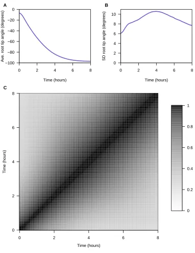
et al.(2013). There are genotype data at 234 markers onﬁve chromosomes; the function-valued root tip angle trait was measured at 241 time points (every 2 min for 8 hr). The estimated genetic map and the trait values forﬁve randomly selected RIL are displayed inSupporting Information,Figure S1. The average and SD of the root tip angle at the individual time points, and the correlations between time points, are displayed inFigure S2.

The data are available at the QTL Archive,http://qtlarchive. org/db/q?pg=projdetails&proj=moore_2013b.

Single-QTL analysis

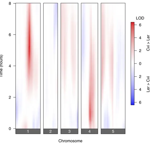
Weﬁrst applied interval mapping by Haley–Knott regression (Haley and Knott 1992), considering each time point indi-vidually. The results are displayed in Figure 1, with thex-axis representing genomic position and they-axis representing time, and so each horizontal slice is a genome scan for one time point. We plot a signed LOD score, with the sign repre-senting the estimated direction of the QTL effect: Red indi-cates that lines with the Cvi allele had a higher phenotype average than the lines with the Ler allele; blue indicates that lines with the Ler allele had a higher phenotype average than the lines with the Cvi allele.

The most prominent QTL are on chromosomes 1 and 4; in both cases the Cvi allele had a higher phenotype value than the Ler allele. The chromosome 1 QTL affects later times, and the chromosome 4 QTL affects earlier times. There is an additional QTL of interest on distal chromosome 3, with the Ler allele having a higher phenotype value at early times.

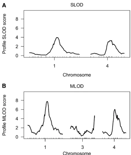
The SLOD and MLOD statistics combine the results across time points, by taking the average or the maximum LOD, respectively, at each genomic location. The results are in Figure 2, A and B. Horizontal lines indicate the 5% genome-wide signiﬁcance thresholds, derived by a permutation test. We also applied the estimating equations approach of Xiong

et al.(2011). This has two variants: a Wald statistic, denoted EE (Wald), and a residual error statistic, denoted EE(Residual). Results are displayed in Figure 2, C and D, again with horizontal lines indicating the 5% genome-wide signiﬁcance thresholds.

The 5% signiﬁcance thresholds for the four methods, derived from permutation tests with 1000 permutation replicates, are shown inTable S1.

All four methods identify QTL on chromosomes 1, 4, and 5. The MLOD and EE(Wald) methods further identify a QTL

Figure 1 Signed LOD scores from single-QTL genome scans, with each

time point considered individually.

Figure 2 (A–D) The SLOD (A), MLOD (B), EE(Wald) (C), and EE(Residual)

(D) curves for the root tip angle data. A red horizontal line indicates the calculated 5% permutation-based threshold.

(4)

on chromosome 3, and the EE(Wald) method identiﬁes a further QTL on chromosome 2.

Multiple-QTL analysis

Methods that account for multiple QTL may improve power and better separate evidence for linked QTL. We extended the approach of Broman and Speed (2002) for function-valued traits. Here we focus on additive QTL models and extend the SLOD and MLOD statistics.

The penalized-SLOD criterion, with the 5% signiﬁcance threshold as the penalty, indicated a two-QTL model with QTL on chromosomes 1 (at 60 cM) and 4 (at 43 cM). The penalized-MLOD statistic indicated a three-QTL model, with an additional QTL on chromosome 3 (at 76.1 cM). The positions of the QTL on chromosomes 1 and 4 were changed slightly relative to the inferred QTL model by the penalized-SLOD criterion; with the penalized-MLOD criterion, the chromosome 1 QTL was at 62 cM and the chromosome 4 QTL was at 39 cM.

Following an approach developed by Zenget al.(2000), we derived profile log-likelihood curves, to visualize the ev-idence and localization of each QTL in the context of a multiple-QTL model: The position of each multiple-QTL was varied one at a time, and at each location for a given QTL, we derived a LOD score comparing the multiple-QTL model with the QTL under con-sideration at a particular position and the locations of all other QTLfixed to the model with the given QTL omitted. This profile is calculated for each time point, individually, and then the SLOD (or MLOD) profiles are obtained by aver-aging (or maximizing) across time points. The SLOD and MLOD profiles are shown in Figure 3.

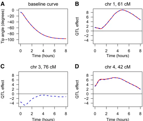
To further characterize the effects of the QTL in the context of the inferred multiple-QTL models, we ﬁtted the selected multiple-QTL models at each time point, individu-ally. For the models derived by the penalized-SLOD and penalized-MLOD criteria, the estimated baseline function and the estimated QTL effects, as a function of time, are shown in Figure 4. The estimated QTL effects in Figure 4, B–D, are for the difference between the Cvi allele and the Ler allele. The estimated effects of the QTL on chromosomes 1 and 4 are approximately the same, whether or not the chromo-some 3 QTL is included in the model. The chromochromo-some 1 QTL has greatest effect at later time points, while the chromosome 4 QTL has greatest effect earlier and over a wider interval of time. For both QTL, the Cvi allele increases the root tip angle phenotype. The chromosome 3 QTL, identiﬁed only with the penalized-MLOD criterion, has an effect at early time points and only for a brief interval of time, and for this QTL, the Ler allele increases the root tip angle phenotype.

Simulations

To investigate the performance of our proposed approaches and compare them to existing methods, we performed several computer simulation studies. While numerous meth-ods for QTL mapping with function-valued traits have been

described, we were unsuccessful, despite considerable ef-fort, to employ the software for Yang et al. (2009), Yap

et al.(2009), Min et al.(2011), or Sillanpääet al.(2012). Thus our main focus for comparison was to the estimating equation approach of Xionget al.(2011). This method has been implemented only for a single-QTL genome scan, and so we compare our approach to that method in the presence of a single QTL. In these single-QTL models, we also consid-ered a simple parametric approach: Fit growth curves for each individual (Kahmet al.2010) and then apply multi-variate QTL analysis (Knott and Haley 2000) with the estimated parameters as phenotypes. In the context of multiple-QTL models, we considered only the two variants of our own approach, the SLOD and penalized-MLOD criteria.

The software used for these simulations is available at http://github.com/kbroman/Paper_FunQTL.

Single-QTL models

To compare our approach to that of Xionget al.(2011) and to a simple parametric approach, in the context of a single-QTL model, we considered the simulation setting described in Yap

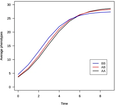
et al.(2009), although exploring a range of QTL effects. We simulated an intercross with sample sizes of 100, 200, or 400 and a single chromosome of length 100 cM with six equally spaced markers and with a QTL at 32 cM. The associated phenotype was sampled from a multivariate nor-mal distribution with the mean curve following a logistic function,gðtÞ ¼a=ð1þbe2rt_Þ_:_{The AA genotype had}_a_{= 29,}

Figure 3 (A and B) SLOD (A) and MLOD (B) proﬁles for a multiple-QTL

(5)

b= 7,r= 0.7; the AB genotype hada= 28.5,b= 6.5,r= 0.73; and the BB genotype hada= 27.5,b= 5,r= 0.75. The shapes of the growth curves with these parameters are shown inFigure S3. Each individual is observed at 10 time points.

The residual error was assumed to be multivariate normal with a covariance structurecS. The constantc con-trols the overall error variance, and S was chosen to have one of three different covariance structures: (1) autoregres-sive withs2_{= 3,}_r_{= 0.6; (2) equicorrelated with}_s2_{= 3,} r = 0.5; or (3) an “unstructured” covariance matrix, as given in Yapet al.(2009) (shown inTable S2).

The parameterc was given a range of values, which

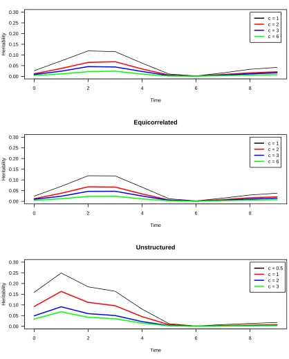
de-ﬁne the percentage of phenotypic variance explained by the QTL (the heritability). The effect of the QTL varies with time; we took the mean heritability across time as an overall summary. For the autoregressive and equicorrelated covari-ance structures, we usedc= 1, 2, 3, 6; for the unstructured covariance matrix, we took c = 0.5, 1, 2, 3. The heritabil-ities, as a function of time, for each covariance structure and for each value of the parameterc, are shown inFigure S4.

For each of 10,000 simulation replicates, we applied our SLOD and MLOD methods, using Haley–Knott regression (Haley and Knott 1992) and the two versions of the method of Xionget al.(2011), EE(Wald) and EE(Residual). We fur-ther applied a simple parametric approach: We fitted the logistic growth model to each individual’s phenotype data, using the R package grofit (Kahmet al.2010), and then used the estimated model parameters as phenotypes, applying the multivariate QTL-mapping method of Knott and Haley (2000). For allfive approaches, wefitted a three-parameter QTL model (that is, allowing for dominance).

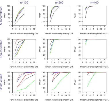
The estimated power to detect the QTL as a function of heritability due to the QTL, for n= 100, 200, 400 and for the three different covariance structures, is shown in Figure 5. With the autocorrelated variance structure, all methods other than the parametric approach gave similar power. With the equicorrelated variance structure, EE(Wald) had higher power than the other four methods, and the para-metric approach was second best. In the unstructured vari-ance setting, the EE(Wald) and MLOD methods worked better than the other three methods. EE(Residual) did not work well in this setting.

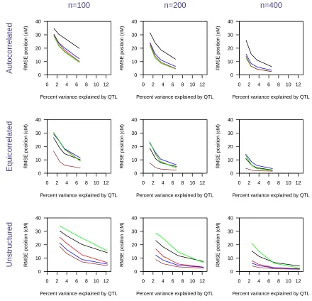
The precision of QTL mapping, measured by the root mean square error in the estimated QTL position, is displayed inFigure S5. Performance, in terms of precision, corresponds quite closely to the performance in terms of power: When power is high, the root mean square error of the estimated QTL position is low, and vice versa.

A possible weakness of the SLOD and MLOD approaches, in not making use of the function-valued form of the phenotypes, is that the methods may suffer lower power in the case of noisy phenotypes. To investigate this possibility, we repeated the simulations withn= 200, adding indepen-dent, normally distributed errors (with standard deviation 1 or 2) at each time point.

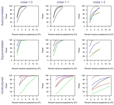
The estimated power to detect the QTL as a function of heritability due to the QTL, for added noise with SD = 0, 1, 2 and the three different covariance structures, is shown in Figure 6. (Corresponding estimates of QTL mapping preci-sion are displayed in Figure S6.) The power of the SLOD, MLOD, and EE(Residual) methods is greatly affected by the introduction of noise. EE(Wald) and the parametric meth-ods are relatively robust to the introduction of noise. Over-all, the EE(Wald) method continued to perform best.

For smooth traits with autocorrelated errors, the SLOD and MLOD methods work similarly to EE(Wald) and EE (Residual). However, if we have large measurement error or have different variance structure, the EE(Wald) method is a robust choice. The parametric approach was more affected by the nature of the residual variance structure than by the addition of random noise.

In terms of computation time, in this simulation study, the MLOD and SLOD methods were3 times faster than EE (Residual), and they were 265 times faster than the EE (Wald) method, withﬁve basis functions used in the latter.

Multiple-QTL models

To investigate the performance of the penalized-SLOD and penalized-MLOD criteria in the context of multiple QTL, we simulated data from the three-QTL model estimated from the root tip angle data of Mooreet al.(2013), considered in theApplicationsection.

We assumed that the mean curve for the root tip angle phenotype followed a cubic polynomial,y=a+bt+ct2₊ dt3_{, and assumed that the effect of each QTL also followed} such a cubic polynomial. Fitting this parametric model with the three penalized-MLOD criterion, we obtained the

Figure 4 (A–D) The regression coefﬁcients estimated for the root tip

angle data set: the estimated baseline function (A) and the estimated QTL effects (B-D). The red curves are for the two-QTL model (from the penalized-SLOD criterion) and the blue dashed curves are for the three-QTL model (from the penalized-MLOD criterion). Positive values for the QTL effects indicate that the Cvi allele increases the tip angle phenotype.

(6)

following estimates. The parameters of the baseline were (a,

b,c,d) = (20.238,2265.248, 229.405,259.771). The QTL

on chromosome 1 at 61 cM had parameters (0.209, 8.729, 1.602,29.054). A second QTL, on chromosome 3 at 76 cM, had parameters (21.887, 3.414,24.220, 2.265). The third QTL, on chromosome 4 at 40 cM, had parameters (2.003, 11.907, 228.647, 15.311). The baseline function and the QTL effect curves are shown in Figure S7.

The four parameters for a given individual were drawn from a multivariate normal distribution with mean deﬁned by the QTL genotypes and variance matrix estimated from the root tip angle data as

S¼ 0 B B @

58:99 2177:77 185:11 245:44 2177:77 3;848:70 27;274:83 3;595:37

185:11 27;274:83 16;897:56 29;702:32 245:44 3;595:37 29;702:32 6;096:71

1 C C A:

In addition, normally distributed measurement error (with mean 0 and variance 1) was added to the phenotype at each time point for each individual. Phenotypes are taken at 241 equally spaced time points in the interval of 0–1. We considered two sample sizes:n= 162 (as in the Mooreet al.

2013 data) and twice that,n= 324.

We performed 2000 simulation replicates. For each repli-cate, we applied a stepwise model selection approach with each of the penalized-SLOD and penalized-MLOD criteria. The simulation results are shown in Table 1.

The penalized-SLOD criterion had higher power to detect theﬁrst and third QTL, while the penalized-MLOD criterion had higher power to detect the second QTL. With the larger sample size, the power to detect QTL increased, and the standard error of the estimated QTL position decreased.

The estimated false positive rates at n= 162 were 3.3 and 0.9% for the penalized-SLOD and penalized-MLOD cri-teria, respectively. At the larger sample size, n= 324, the corresponding false positive rates were 4.1 and 0.8%.

Discussion

Automated phenotype measurement is an accelerating trend across biological scales, from microorganisms to crop plants. This push for increasing automation makes it feasible to increase the dimensionality of phenotype data sets, for example by adding time. The trend toward higher-dimensional phenotype data sets from genetically structured populations has created a need for new statistical genetic methods, and computational speed can be an important factor in the ap-plication of such methods.

Figure 5 Power as a function of

(7)

Methods for the genetic analysis of function-valued phenotypes have mostly focused on single-QTL models (Ma et al. 2002; Yang et al. 2009; Yapet al. 2009; Xiong

et al.2011). Bayesian multiple-QTL methods, using Markov chain Monte Carlo, have also been proposed (Min et al.

2011; Sillanpää et al.2012), but they can be computation-ally intensive and not easily implemented. We propose two simple LOD-type statistics that integrate the information across time points and extend them, using the approach of Broman and Speed (2002), for multiple-QTL model selection.

The basis of our approach is the analysis of each time point individually. This works well when the function-valued trait is smooth, as in the data from Mooreet al.(2013), and has the benefit of providing results that are easily inter-preted, such as the QTL effects displayed in Figure 4. With unequally spaced time points or appreciable missing data, the approach may require some modification, such asfirst performing some interpolation or smoothing. The perfor-mance of our approaches deteriorated with added noise, but again this may be at least partly alleviated by pre-smoothing. An important advantage of our approach is the ability to incorporate information from multiple QTL in the analysis of function-valued phenotypes, which should im-prove power and lead to better separation of linked QTL.

A weakness of our approach is that it largely ignores the correlations across time. Ma et al. (2002) and Yang et al.

(2009) paid careful attention to this aspect, using an auto-regressive model for the residual variance matrix. Our cur-rent neglect of this aspect may result in loss of efﬁciency, particularly in the estimates of the QTL effects. However, by ignoring this assumption we gain much speed, and our sim-ulation studies indicate that the approach exhibits reason-able power to detect QTL in many situations. The EE(Wald) method of Xionget al.(2011) showed the best performance among all methods considered, although at the expense of considerably greater computation time.

Figure 6 Power as a function of

the percentage of phenotypic vari-ance explained by a single QTL, with additional noise added to the phenotypes. The left column has no additional noise; the center and right columns have indepen-dent normally distributed noise added at each time point, with standard deviations 1 and 2, re-spectively. The three rows corre-spond to the covariance structure (autocorrelated, equicorrelated, and unstructured). In each panel, SLOD is in red, MLOD is in blue, EE(Wald) is in brown, EE(Residual) is in green, and parametric is in black. The per-centage of variance explained by the QTL on the x-axis refers, in each case, to the variance explained in the case of no added noise.

Table 1 Simulation results for the SLOD and MLOD criteria, for

a three-QTL model, modeled after the Mooreet al.(2013) data

Mean (SE) estimated location Power

n True location SLOD MLOD SLOD MLOD

162 61 60.7 (6.7) 61.0 (5.4) 88.7 54.5

76 64.4 (18.9) 71.1 (12.2) 11.8 14.6 40 39.9 (5.2) 40.0 (3.4) 82.0 76.9

324 61 61.1 (4.2) 61.2 (4.3) 100 58.7

76 71.9 (9.8) 74.4 (5.8) 30.7 43.3 40 39.9 (2.6) 40.1 (2.0) 99.8 91.1

Note that locations are in centiMorgans.

(8)

Manichaikul et al.(2009) extended the work of Broman and Speed (2002) by considering pairwise interactions among QTL. Our approach may be similarly extended to consider interactions.

An alternative approach to the QTL analysis of function-valued traits is to first fit a parametric model to each individual’s curve and then treat the estimated parameters from such a model as phenotypes. (The method exhibited less-than-ideal performance in our simulation study, likely due to poor modelfit with the simulated error structures.) Multiple-QTL mapping methods could readily be applied to each such parameter, individually. The advantage of our ap-proach, to consider each time point individually, is in the simpler interpretation of the results.

Software implementing our methods have been imple-mented as a package for R (R Core Team 2013), funqtl (https://github.com/ikwak2/funqtl).

Acknowledgments

The authors thank ´Saunak Sen and two anonymous reviewers for comments to improve the manuscript. This work was sup-ported in part by grant IOS-1031416 from the National Science Foundation Plant Genome Research Program (to E.P.S.) and by National Institutes of Health grant R01GM074244 (to K.W.B.).

Literature Cited

Broman, K. W., and T. P. Speed, 2002 A model selection approach for the identiﬁcation of quantitative trait loci in experimental crosses. J. R. Stat. Soc. B 64: 641–656.

Churchill, G. A., and R. W. Doerge, 1994 Empirical threshold values for quantitative trait mapping. Genetics 138: 963–971. Dempster, A., N. Laird, and D. Rubin, 1977 Maximum likelihood from

incomplete data via the EM algorithm. J. R. Stat. Soc. Ser. B 39: 1–38. Haley, C. S., and S. A. Knott, 1992 A simple regression method for mapping quantitative trait loci in line crosses using ﬂanking markers. Heredity 69: 315–324.

Kahm, M., G. Hasenbrink, H. Lichtenberg-Fraté, J. Ludwig, and M. Kschischo, 2010 groﬁt: Fitting biological growth curves with R. J. Stat. Softw. 33: 1_–21.

Kendziorski, C. M., A. W. Cowley, A. S. Greene, H. C. Salgado, H. J. Jacobet al., 2002 Mapping baroreceptor function to ge-nome: a mathematical modeling approach. Genetics 160: 1687–1695.

Knott, S. A., and C. S. Haley, 2000 Multitrait least squares for quantitative trait loci detection. Genetics 156: 899–911. Lander, E. S., and D. Botstein, 1989 Mapping Mendelian factors

underlying quantitative traits using RFLP linkage maps. Genet-ics 121: 185–199.

Ma, C., G. Casella, and R. L. Wu, 2002 Functional mapping of quantitative trait loci underlying the character process: a theo-retical framework. Genetics 161: 1751–1762.

Manichaikul, A., J. Y. Moon, S. Sen, B. S. Yandell, and K. W. Broman, 2009 A model selection approach for the identi_ﬁcation of quan-titative trait loci in experimental crosses, allowing epistasis. Genetics 181: 1077–1086.

Min, L., R. Yang, X. Wang, and B. Wang, 2011 Bayesian analysis for genetic architecture of dynamic traits. Heredity 106: 124–133. Moore, C. R., L. S. Johnson, I.-Y. Kwak, M. Livny, K. W. Broman

et al., 2013 High-throughput computer vision introduces the time axis to a quantitative trait map of a plant growth response. Genetics 195: 1077–1086.

R Core Team, 2013 R: A Language and Environment for Statistical Computing. R Foundation for Statistical Computing, Vienna. Sillanpää, M. J., P. Pikkuhookana, S. Abrahamsson, T. Knurr, A.

Frieset al., 2012 Simultaneous estimation of multiple quanti-tative trait loci and growth curve parameters through hierarchi-cal Bayesian modeling. Heredity 108: 134_–146.

Xiong, H., E. H. Goulding, E. J. Carlson, L. H. Tecott, C. E. McCulloch

et al., 2011 Aﬂexible estimating equations approach for map-ping function-valued traits. Genetics 189: 305–316.

Yang, J., R. L. Wu, and G. Casella, 2009 Nonparametric functional mapping of quantitative trait loci. Biometrics 65: 30–39. Yap, J. S., J. Fan, and R. Wu, 2009 Nonparametric modeling of

longitudinal covariance structure in functional mapping of quantitative trait loci. Biometrics 65: 1068–1077.

Zeng, Z. B., J. J. Liu, L. F. Stam, C. H. Kao, J. M. Merceret al., 2000 Genetic architecture of a morphological shape difference between two Drosophila species. Genetics 154: 299_–310.

(9)

GENETICS

Supporting Information

http://www.genetics.org/lookup/suppl/doi:10.1534/genetics.114.166306/-/DC1

A Simple Regression-Based Method to Map

Quantitative Trait Loci Underlying

Function-Valued Phenotypes

Il-Youp Kwak, Candace R. Moore, Edgar P. Spalding, and Karl W. Broman

(10)

100

80

60

40

20

0 Chromosome

Location (cM)

1

2

3

4

5 A

2

4

6

8 −120

−100

−80

−60

−40

−20

0 Time (hours)

Root Tip Angle (degrees)

B

Figure S1 Gene c map of typed gene c markers (A) and func on-valued phenotypes for ﬁve randomly selected Arabidopsis

(11)

0 2 4 6 8 −100

−80 −60 −40 −20 0

Time (hours)

A

v

e

. root tip angle (degrees)

A

0 2 4 6 8

0 2 4 6 8 10

Time (hours)

SD root tip angle (degrees)

B

Time (hours)

C

0 2 4 6 8

0 0.2 0.4 0.6 0.8 1

Figure S2 Average (A) and standard devia on (B) of the root p angle phenotype at each individual me point, and the

correla ons between me points (C).

(12)

0

2

4

6

8

0

5

10

15

20

25

30 Time

A

v

er

age phenotypes

0

2

4

6

8

0

5

10

15

20

25

30 Time

A

v

er

age phenotypes

0

2

4

6

8

0

5

10

15

20

25

30 Time

A

v

er

age phenotypes

BB

AB

AA

(13)

0 2 4 6 8 0.00

0.05 0.10 0.15 0.20 0.25 0.30

Autocorrelated

Time

Her

itability

c = 1 c = 2 c = 3 c = 6

0 2 4 6 8

0.00 0.05 0.10 0.15 0.20 0.25 0.30

Equicorrelated

Time

Her

itability

c = 1 c = 2 c = 3 c = 6

0 2 4 6 8

0.00 0.05 0.10 0.15 0.20 0.25 0.30

Unstructured

Time

Her

itability

c = 0.5 c = 1 c = 2 c = 3

Figure S4 The heritability for each me point in the single-QTL simula on study, for the three assumed variance structures

and the chosen values for thecparameter.

(14)

0 2 4 6 8 10 12 0

10 20 30 40

Percent variance explained by QTL

RMSE position (cM)

A

utocorrelated

n=100

0 2 4 6 8 10 12

0 10 20 30 40

RMSE position (cM)

n=200

0 2 4 6 8 10 12

0 10 20 30 40

RMSE position (cM)

n=400

0 2 4 6 8 10 12

0 10 20 30 40

RMSE position (cM)

Equicorrelated

0 2 4 6 8 10 12

0 10 20 30 40

RMSE position (cM)

0 2 4 6 8 10 12

0 10 20 30 40

RMSE position (cM)

0 2 4 6 8 10 12

0 10 20 30 40

RMSE position (cM)

Unstr

uctured

0 2 4 6 8 10 12

0 10 20 30 40

RMSE position (cM)

0 2 4 6 8 10 12

0 10 20 30 40

RMSE position (cM)

Figure S5 Root Mean Square Error (RMSE) of the es mated QTL posi on as a func on of the percent variance explained by

(15)

0 2 4 6 8 10 12 0

10 20 30 40

RMSE position (cM)

A

utocorrelated

noise = 0

0 2 4 6 8 10 12

0 10 20 30 40

RMSE position (cM)

noise = 1

0 2 4 6 8 10 12

0 10 20 30 40

RMSE position (cM)

noise = 2

0 2 4 6 8 10 12

0 10 20 30 40

RMSE position (cM)

Equicorrelated

0 2 4 6 8 10 12

0 10 20 30 40

RMSE position (cM)

0 2 4 6 8 10 12

0 10 20 30 40

RMSE position (cM)

0 2 4 6 8 10 12

0 10 20 30 40

RMSE position (cM)

Unstr

uctured

0 2 4 6 8 10 12

0 10 20 30 40

RMSE position (cM)

0 2 4 6 8 10 12

0 10 20 30 40

RMSE position (cM)

Figure S6 Root Mean Square Error (RMSE) of the es mated QTL posi on as a func on of the percent variance explained by

a single QTL, with addi onal noise added to the phenotypes. The ﬁrst column has no addi onal noise; the second and third columns have independent normally distributed noise added at each me point, with standard devia on 1 and 2, respec vely. The three rows correspond to the covariance structure (autocorrelated, equicorrelated, and unstructured). In each panel, SLOD is in red, MLOD is in blue, EE(Wald) is in brown, EE(Residual) is in green, and parametric is in black. The percent variance explained by the QTL on the x-axis refers, in each case, to the variance explained in the case of no added noise.

(16)

0.0 0.2 0.4 0.6 0.8 1.0

−100

−80

−60

−40

−20

0 Time

Root Tip Angle

baseline curve

A

0.0 0.2 0.4 0.6 0.8 1.0

−4

−2

0

2

4 Time

QTL eff

ect

chr 1, 61 cM

B

0.0 0.2 0.4 0.6 0.8 1.0

−4

−2

0

2

4 Time

QTL eff

ect

chr 3, 76 cM

C

0.0 0.2 0.4 0.6 0.8 1.0

−4

−2

0

2

4 Time

QTL eff

ect

chr 4, 42 cM

D

(17)

Table S1 5% signiﬁcance thresholds for the data from Mooreet al.2013, based on a permuta on test with 1000 replicates.

Method Threshold

SLOD 1.85

MLOD 3.32

EE(Wald) 5.72

EE(Residual) 0.0559

(18)

Table S2 The unstructured covariance matrix used in the single-QTL simula ons.

Σ =                

0.72 0.39 0.45 0.48 0.50 0.53 0.60 0.64 0.68 0.68 0.39 1.06 1.61 1.60 1.50 1.48 1.55 1.47 1.35 1.29 0.45 1.61 3.29 3.29 3.17 3.09 3.19 3.04 2.78 2.53 0.48 1.60 3.29 3.98 4.07 4.01 4.17 4.18 4.00 3.69 0.50 1.50 3.17 4.07 4.70 4.68 4.66 4.78 4.70 4.36 0.53 1.48 3.09 4.07 4.68 5.56 6.23 6.87 7.11 6.92 0.60 1.55 3.19 4.17 4.66 6.23 8.59 10.16 10.80 10.70 0.64 1.47 3.04 4.18 4.78 6.87 10.16 12.74 13.80 13.80 0.68 1.35 2.78 4.00 4.70 7.11 10.80 13.80 15.33 15.35 0.68 1.29 2.53 3.69 4.36 6.92 10.70 13.80 15.35 15.77