Frequency-aware Static Timing Analysis for Power-aware Embedded Architectures

(1)

Seth, Kiran R. Frequency-aware Static Timing Analysis for Power-aware Embed-ded Architectures (Under the direction of Assistant Professor Dr. Frank Mueller). Power is a valuable resource in embedded systems as the lifetime of many such systems is con-strained by their battery capacity. Recent advances in processor design have added support for dynamic frequency/voltage scaling (DVS) for saving power. Recent work on real-time scheduling focuses on saving power in static as well as dynamic scheduling environments by exploiting idle and slack due to early task completion for DVS of subsequent tasks. These scheduling algorithms rely on a priori knowledge of worst-case execution times (WCET) for each task. They assume that DVS has no effect on the worst-case execution cycles (WCEC) of a task and scale the WCET according to the processor frequency. However, for systems with memory hierarchies, the WCEC typically does change under DVS due to frequency modulation. Hence, current assumptions used by DVS schemes result in a highly exaggerated WCET.

(2)

by

Kiran R. Seth

A thesis submitted to the Graduate Faculty of North Carolina State University

in partial satisfaction of the requirements for the Degree of

Master of Science in Computer Engineering

Department of Electrical and Computer Engineering

Raleigh

2003

Approved By:

Dr. Alexander Dean Dr. Eric Rotenberg

(3)

Biography

(4)

Acknowledgements

(5)

List of Figures

2.1 Actual vs. Assumed WCEC for fft . . . 6

2.2 Actual vs. Assumed WCET for fft . . . 7

3.1 Sample Instruction Sequence . . . 9

3.2 Ex 1: Perfect run of instruction sequence . . . 10

3.3 Ex 2: Instruction cache miss . . . 10

3.4 Ex 3: Data cache miss . . . 11

3.5 Ex 4: Instruction + data cache miss . . . 11

4.1 Obtaining Safe WCET Bounds . . . 14

5.1 FAST-Static Voltage Scaling for EDF . . . 21

5.2 FAST-Cycle conserving DVS for EDF . . . 22

5.3 FAST-Look ahead DVS for EDF . . . 24

6.1 FAST vs. Traditional WCEC . . . 28

6.2 Exp 2a: Energy Normalized to Base EDF for Various Task Sets . . . 36

(8)

Chapter 1

Introduction

This chapter introduces the area of real-time systems and stresses the importance of static timing analysis to calculate the Worst-Case Execution Time (WCET) for real-time applications. Scheduling algorithms for low-power real-time systems are introduced along with some deficiencies in the algorithms.

1.1 Worst-Case Execution Time

Real-time systems are systems where the correct operation of the system depends not only on logical correctness of the input/output relation, but also on the timeliness of the system. Each task executing on a real-time system has a definite deadline that it must meet. Depending on the penalty of missing the deadline, real-time systems can be classified into hard real-time systems (catastrophic results when missing deadlines) and soft real-time systems (quality of service suffers due to missed deadline). To schedule tasks on a real-time system, an accurate bound of the execution time for the tasks is required.

Schedulability tests based on real-time theory depend on safe upper bounds on the WCET to guarantee that deadlines are met [22, 8, 29]. Bounds on the WCET should also be as tight as possible. A lax WCET bound may result in an underutilized system consuming excess energy or providing excess processing power and, thereby, raising cost. Safe and tight WCET bounds can be provided by static timing analysis for relatively simple, scalar architectures with in-order execution and static branch prediction (if any branch prediction at all), and split caches [26, 21, 2, 19, 17, 30, 15, 23, 25].

(9)

the WCET of a real-time task. Conventional methods for static analysis have been extended from unoptimized programs on simple CISC processors to optimized programs on pipelined RISC processors , and from uncached architectures to instruction and data caches [26, 21, 16, 25, 33, 20]. The challenge of static timing analysis is to provide not only safe but also tight bounds on the WCET in order to impose a high enough processor utilization. These analysis approaches result in tight bounds for deterministic microarchitectures with simple components.

1.2 Dynamic Voltage Scaling

Limitations on the lifetime of embedded devices, particularly battery-powered mo-bile devices, have resulted in advances in embedded architecture to extend the lifetime of devices. Microprocessor designs ranging from low-end 8-bit up to high-end 32-bit embedded architectures (e.g., the Atmel Atmega AVR family on the low end and the Intel XScale on the high-end, just to name two extremes) support dynamic adjustment of processing speed to prolong battery life. Generally, two techniques are employed in unison. On one side, dynamic frequency scaling allows the speed of instruction execution to change during the operation of a device. On the other side, dynamic voltage scaling modulates the level of the supply voltage upon demand. Generally, both schemes, referred to as DVS in the fol-lowing, work hand in hand: When the frequency is lowered by a certain degree, the voltage can be also be reduced to a lower level. Furthermore, both scaling techniques impact the power consumption of a device: power scales linearly with the frequency and quadratically with the voltage. Hence, considerable power savings may result in a concerted approach of dynamic frequency and voltage scaling [10].

(10)

Recently, a number of hard real-time DVS scheduling schemes have been studied, ranging from compiler support [24] over numerous static scheduling approaches [14, 27] to dynamic methods [27, 3, 13]. All of these approaches have their own merits in that they provide a solution suitable to certain systems depending on scheduling methods, utilization bounds of the task sets and architectural properties, such as scaling overhead.

Any DVS scheduling scheme is subject to the same constraints as other hard real-time systems: The worst-case execution real-time (WCET) of a task has to be knowna priori,

i.e., safe bounds on a task’s execution time have to be obtained. Prior work on static timing analysis provides the means to derive relatively tight WCET bounds for simple embedded architectures, which are provably safe.

In the context of DVS, static timing analysis is generally assumed to remain valid with frequency scaling. The conjecture is that reducing a processor’s frequency still results in thesame number of cycles of execution for a task. Hence, considering the processor fre-quency should suffice to derive safe WCET bounds. However, this simplistic view generally

does not hold for any realistic architectures. Consider the impact of memory references.

Any instruction or data reference that is resolved through a main memory access operates at external bus frequency. But bus frequencies generally diverge from internal processor frequencies, and they do not scale at the same rate as DVS scaling does. E.g., the first generation Compaq Ipaq has a StrongArm microprocessor (SA-1110) that scales at 8 fre-quencies but only supports two different external bus frefre-quencies.

(11)

dynamic scheduling, preemption and early completion.

1.3 Parametric Frequency Model

The contribution of this thesis is to remedy this problem by promoting a new methodology for frequency-aware static timing analysis (FAST). Instead of obtaining a WCET bound for each frequency pair, FAST takes static timing analysis to a novel level suitable for dynamic scheduling. FAST expresses WCET bounds as a parametric term whose components are frequency-sensitive parameters. On the one side, cycles are interpreted in terms of the processor frequency; on the other hand, memory accesses are expressed in terms of the memory latency overhead due to the external bus speed. This parametric expression of the WCET allows one to determine on-the-fly the WCET for a given frequency pair. This is particularly appealing when scheduling decisions occur dynamically and when the number of frequency pairs becomes large, such as is the case with state-of-the-art processors with fine-grained frequency settings.

1.4 Outline

(12)

Chapter 2

Effects of frequency scaling on

WCET

In this chapter, the effects of frequency modulation on the WCET of applications are discussed. The motivation for a parametric frequency model is also explained along with the challenges of supporting the novel model in a static timing analysis tool.

(13)

0 500000 1000000 1500000 2000000 2500000 3000000

100 175 250 325 400 475 550 625 700 775 850 925

Frequency (MHz)

N

u

m

b

e

r

o

f

C

y

c

le

s

Actual WCEC Assumed WCEC

Figure 2.1: Actual vs. Assumed WCEC for fft

upon frequency scaling the non-memory instructions would require the same number of cy-cles for execution. But the number of cycy-cles required to execute the memory referencing instructions changes, depending on the current processor frequency and the constant FSB frequency. Usually, a decrease in the frequency decreases the number of cycles required to access the memory. By assuming that the WCEC remains constant, one ignores the fact that the WCECreduceswith frequency, which results in WCET overestimations.

(14)

0 5 10 15 20 25 30

100 175 250 325 400 475 550 625 700 775 850 925

Frequency (MHz)

T

im

e

(

m

s

)

Actual WCET Assumed WCET

Figure 2.2: Actual vs. Assumed WCET for fft

control the accuracy of the WCEC, but they also affect the accuracy by which the WCEC can be scaled with frequency. Figure 2.2 depicts the equivalent WCET to the two WCEC curves in Figure 2.1. The actual WCET depicted indicates the assumption of a constant WCEC independent of frequency modulations result in considerable overestimations of the WCET.

(15)

Chapter 3

Parametric Frequency Model

In this chapter, the parametric frequency model is discussed. The frequency model can be used to estimate the WCET in the form of a parametric equation allowing the calculation of accurate WCET with the change in frequency.

The proposed parametric frequency model can be used for timing analysis with any simple in-order single-issue pipeline. The model is applicable to systems with or without a memory hierarchy. A system without memory hierarchy (without caches) behaves just like a system with a memory hierarchy where all the memory accesses are misses. The parametric frequency model can also be applied to a system without caches. The examples consider the model in a system with a memory hierarchy, and solutions are contributed to the technical challenges posed. It is assumed that the system is equipped with an on-chip instruction and data cache and that the main external memory has a constant access latency. To accurately model the WCET in systems with memory hierarchies, the parametric frequency model is proposed, that can captures the effect of frequency scaling accurately by splitting the WCEC of a task into two components. The first component,i, captures the ideal number of cycles required to execute the task assuming perfect caches. In other words,idoes not scale with frequency. The second component, m, counts the total number of instruction and data cache misses for the task. m is the part of the WCEC that scales with frequency and depends on the memory access latency. If a system without caches is considered, iwould count the total number of cycles used for non-memory operations whilem would count the total number of memory references. Thus, the WCEC is expressed as follows:

(16)

A:

add R2, R1, R3

B:

load R4, [M1]

C:

add R2, R1, R4

D:

add R2, R1, R5

Figure 3.1: Sample Instruction Sequence

where N is the number of cycles required to access the memory, which depends on the latency of the memory L and the frequency f of the processor. Therefore, we may also express Equation 3.1 in terms of frequency as shown in Equation 3.2. Thus WCEC is expressed as a function of the frequency.

W CEC =i+mLf (3.2)

For a simple pipeline, the WCEC can be easily be converted into the WCET by dividing by the frequency. This frequency model can accurately model the actual WCET because it separates the WCEC into components, one that scales and one that does not scale with processor frequency.

The following examples are presented to show that the parametric model can cap-ture the effects of different sequences of instructions in a task. Only sequences that contain data or instruction cache misses are of concern since they are affected during frequency scaling. A sequence of instructions without any cache misses can be captured exclusively by theicomponent and represents a trivial example for the parametric model. For the fol-lowing examples, let N = 10, as shown in the figures below. Separate instruction and data caches are assumed and frequency scaling for the model with an arbitrary simple in-order pipeline.

Consider a sequence of four instructions, as shown in the Figure 3.1.

This instruction sequence is executed in a processor with a simple six-stage in-order pipeline. The pipeline stages are fetch (IF), decode (ID), issue (IS), execute (EX), memory access (MEM) and write-back (WB).

(17)

Cycles

IF

ID

IS

EX

MEM

WB

2

3

4

5

1

6 A

A

B

C

D

C

D

C

D

C

B

B C

D

C

D

7

8

9

Figure 3.2: Ex 1: Perfect run of instruction sequence

2. In Figure 3.3, observe the effects of an instruction cache. Consider instruction B resulting in a miss. While instruction B misses in the instruction cache, all other cache accesses result in hits. Since instructions are stalled till the miss on B is resolved, the number of cycles involved can be separated into two components. With i = 9 and m = 1 in Equation 3.1, the WCEC is accurately captured by the model as W CEC = 9 + 1N. Hence, the WCEC is accurately modeled for any value of N resulting in an accurate WCET regardless of frequencies.

3. In Figure 3.4, observe the effects of a data cache miss. Instruction B misses in the data cache while all other cache accesses are hits. Withi= 9 andm= 1, the WCEC

Cycles

IF

ID

IS

EX

MEM

WB

2

3

4

5

1

6 −

− 12 13 14 15 16 17 18 19

A

B

−

B

C

D

(18)

Cycles

IF

ID

IS

EX

MEM

WB

2

3

4

5

1

6 −

−

A

B

C

D

C

D

C

D

C

16 17 18 19

D

C

D

C

B

−

B

−

B

C

Figure 3.4: Ex 3: Data cache miss

is again calculated as 9 + 1N. Since the data miss stalls the previous instructions, one can separate the number of cycles required for the memory access. However, had the Instruction C or any other stalled instruction performed any useful work instead of being stalled, a potential for overestimation would occur for the model,e.g., for multi-cycle floating-point operations, branch mispredictions, etc. Any such overestimation results from the overlap of useful cycles with the memory stall. In the model, the i component counts these useful cycles while the m component counts data miss. Overlap would not be considered by the model. For example, if instruction C took an extra cycle to execute, the new WCEC would become 10 + 1N. The model does not

Cycles

IF

ID

IS

EX

MEM

WB

2

3

4

5

1

6 −

−

A

B

−

D

C

B

D

C

D

C

D

C

D

C

D

C

B

C

−

C

−

13 14 15 16

24 25 26 27

B

C

(19)

consider the overlap between the data miss and the extra cycle used by instruction C. A similar problem is also observed in example 1 if the instruction miss overlaps with a high execution latency instruction.

The potential for overestimations implies that the obtained WCET obtained still provides an upper bound on the execution time, albeit not necessarily a tight one. But removing overestimations due to instructions with high execution latencies is non-trivial because instructions may have different execution latencies. Subsequent experiments show that these design choices have a diminishing affect on the tightness of WCET bounds.

4. In Figure 3.5, observe the effects of a simultaneous instruction and data cache misses. Instruction B results in a data cache miss while the instruction C results in an in-struction cache miss. All other cache accesses are hits. With i = 9 and m = 2, the W CEC = 9 + 2N. The instruction and the data cache misses cannot be serviced together. Hence, instruction B is stalled till instruction C’s cache miss is serviced. The model captures all sequences of instructions where a cache miss stalls yet another cache miss. Notice that the two misses in question need not result from consecutive instructions. Some overestimation is observed because of overlapping of some work with the miss cycles.

(20)

Chapter 4

Timing analysis for Real-time

applications

In this chapter, conventional static timing analysis is described and the approach is briefly contrasted to dynamic timing analysis methods. Novel enhancements, necessitated by DVS, are specified to adapt conventional static timing analysis to a frequency-aware static timing analysis (FAST) tool.

4.1 Static Timing Analysis

Schedulability analysis for hard real-time systems requires that the worst-case execution time (WCET) be safely bounded in order to ensure feasibility of scheduling a task set for a given scheduling policy, such as rate-monotone and earliest-deadline-first scheduling [22]. If the execution time of a task were obtained through dynamic timing analysis based on experimental or trace-driven approaches, these values would not provide a safe bound of the WCET [32]. On the one side, it is difficult to determine the worst-case input set even for moderately complex tasks that would exhibit the WCET, and to perform exhaustive testing over the entire input space is infeasible except for trivial cases. On the other side, even if the worst-case input set was known, the interaction between the software and hardware might cause the task to exhibit its WCET for a different input set. The cause of this behavior is architectural complexity, such as complex pipelines and caching mechanisms.

(21)

various static approaches have been studied, this research will constrains itself to one such toolset without loss of generality [15, 25, 33]. The WCET bounds obtained by static tim-ing analysis provide a guaranteed upper bound on the computation time of a task. Static timing analysis performs the equivalent of a traversal over all execution paths to determine timing information independent of a program trace and without tracking values or program variables. Loop bodies only require a few traversals to determine the worst-case behavior of the entire loop due to an efficient fixed-point approach. As the execution paths are tra-versed, the behavior of the architectural components along the execution paths is captured. The paths are composed to form loops, functions and ultimately the entire application to calculate both WCEC and WCET.

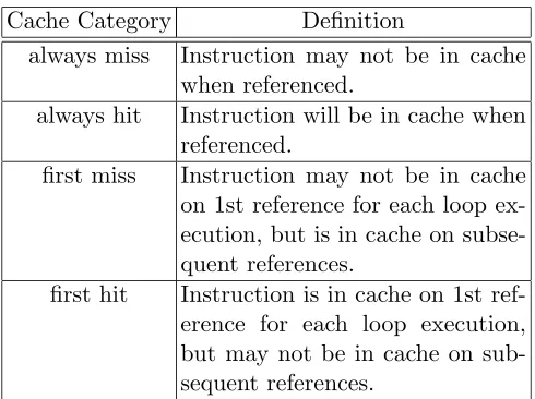
Figure 4.1 depicts an overview of the organization of this timing analysis toolset. An optimizing compiler has been modified to produce control flow and branch constraint information as a side effect of the compilation of a source file. The original research compiler VPCC/VPO [4] was replaced by GCC with a Portable Instruction Set Architecture (PISA) backend that interfaces with SimpleScalar. Real-time applications are compiled into assem-bly code using the GCC PISA-compiler. The control-flow graph and instruction as well as data references are extracted from the assembly code. Upper bounds on the number of iterations performed by loops are provided, a prerequisite for performing static timing anal-ysis. A static instruction cache simulator uses the control flow information to construct a control-flow graph of the program that consists of the call graph and the control flow of each function. The program’s control-flow graph is then analyzed, and a caching categorization for each instruction and data reference in the program is produced. Separate categorizations are provided for each loop level in which the instructions and data references are contained. The categorizations for instruction references are described in Table 4.1. Next, the

tim-Source Files

Simulator Cache

Static _Cache

Categorization Analyzer

Timing WCET Prediction Control Flow &

I/D−References Gcc (PISA)

Compiler

(22)

ing analyzer uses the control flow and constraint information, caching categorizations, and machine dependent information (e.g., pipeline characteristics) to calculate bounds on the WCET.

Cache Category Definition

always miss Instruction may not be in cache when referenced.

always hit Instruction will be in cache when referenced.

first miss Instruction may not be in cache on 1st reference for each loop ex-ecution, but is in cache on subse-quent references.

first hit Instruction is in cache on 1st ref-erence for each loop execution, but may not be in cache on sub-sequent references.

Table 4.1: Instruction Categories for WCET

This approach differs from prior toolset in [1]. The tool separates static I-cache and D-cache (instruction/data cache) analysis. The D-cache analysis currently lacks sufficiently detailed information about references for the GCC compilation phase, and D-cache analysis does not fully match the SimpleScalar model. The focus of this research is on enhancing the timing analyzer with respect to the FAST model and PISA instruction set. But since the SimpleScalar-based architectural simulation environment [28] is used to validate the approach, simplifying assumptions about the data caches have to be made. Specifically, it is assumed that a constant number of data cache accesses to be misses for each application to model compulsory misses. The remaining references are considered to be hits, which models a sufficiently large cache.

(23)

paths through a loop body or a function. Static branch prediction is easily accommodated by worst-case analysis: the misprediction penalty is added to the non-predicted path (not-taken path for backward branches and (not-taken path for forward branches). Path analysis (see below) selects the longest execution path as usual. Once timings for alternate paths in a loop are obtained, a fixed-point algorithm (quickly converging in practice), is employed to safely bound the time of the loop based on the its body’s cycle counts.

The fixed-point approach generally requires path analysis for only a few iterations. Given the longest path for the first iteration, the next-longest path is determined for the second iteration, which may differ from the original path due to caching effects. The lengths of these paths are monotonically decreasing due to cache effects, and once a fixed-point is reached, subsequent loop iterations can be safely approximated by this fixed-point timing value. When the longest paths of consecutive iterations are combined, the tool accounts for the pipeline overlap between the tail of the earlier path and the head of the path that follows. The alternative – no overlap – is tantamount to draining the pipeline between iterations. Using this fixed-point approach, the timing analyzer ultimately derives WCET bounds, first for each path, then for loops, and finally for functions within the program. A timing analysis tree is constructed, where each node of the tree corresponds to a loop or function. Nodes in the tree are processed in a bottom-up manner. In other words, the WCET for an outer loop / caller is not calculated until the times for all of its inner loops / callees are known. This means that the timing analyzer predicts the WCET for programs by first analyzing the innermost loops and functions before proceeding to higher-level loops and functions, eventually reaching the tree’s root (e.g., main()). The timing analysis tree provides a convenient method for obtaining WCET for a specific scope. From the description in this section, it becomes evident that static timing analysis is non-trivial, even for simple pipelines.

4.2 Frequency-Aware Static Timing Analysis

(24)

the change in memory latency, the WCEC information for different paths changes, which may result in a different worst-case path than before. The frequency model can be elegantly incorporated into static timing analysis such that it calculates the number of cycles foreach

possible worst-case path in the program. The following technical innovations to the static

timing analysis framework support such flexible calculations.

Instead of using the memory access cycles to simulate the sequence of instructions in the pipeline, the ideal number of cycles is calculated assuming all cache accesses to be hits. The instruction and data cache misses are accumulated as a side-effect to compose a first-order polynomial equation describing the WCEC.

Static timing analysis requires different paths through the same node (loop or function) to be compared. The path with the worst WCEC is used as the WCEC for the node. After integrating the frequency model into the framework, one has to compare two equations to determine which one was to result in a larger number of execution cycles. The challenge here is posed by having to consider both equations: One of them has greater WCEC for some range of frequencies while the other has greater WCEC for the rest of the frequency range. Remember that the frequency model is a first-order polynomial. Consider the case where two equations intersect, i.e., both polynomial have a common solution. Three approaches to address this problem are proposed.

1. One can maintain an ordered list of equations and the ranges where subsequent poly-nomials represent a larger WCEC than previous ones. Since the frequency model is a first-order polynomial with different slopes, there exists an intersection point constraining the range for each equation.

2. Alternatively, a curve-fitting equation could capture the effects of both equations. This obviates the need for maintaining large numbers of equations but increases the complexity of the parametric equation. A higher-order polynomial with strict upper bounds on each base polynomial would provide a relatively close fit. The resulting curve would not be as tight as in case (1) but may suffice if the slopes of the original polynomials do not diverge significantly. This would impose more overhead on dy-namic scheduling schemes that have to perform additional arithmetic to evaluate the equation upon any scheduling action.

(25)

two equations intersect outside the given range, the equation that provides the higher WCEC within the valid range can be chosen. If two equations intersect within this specified range, a simple curve-fitting technique through a first-order polynomial that provides a WCEC greater or equal to the values of either of the original equations can be used.

(26)

Chapter 5

Applying FAST framework to DVS

schemes

In this chapter, FAST equations for WCET are incorporated into existing DVS-EDF scheduling algorithms as proposed by Pillai and Shin through (a) static voltage scaling, (b) cycle-conserving RT-DVS and (c) look-ahead RT-DVS [27]. With only minimal changes to the original algorithms, the FAST equations can be integrated into the respective DVS schemes, thereby improving energy savings obtained.

5.1 FAST-EDF Utilization

Most DVS scheduling algorithms use the assumption that the WCEC is constant with frequency when scaling the WCET. By not considering the effect on WCEC during frequency modulation, DVS schemes assume a considerably overestimated WCET. Thus, DVS schemes fail to completely utilize available slack because the scaled WCET is not a tight bound. The parametric frequency model is implemented in the FAST framework. Parametric equations obtained by FAST can be used in DVS scheduling schemes to ensure that the scaled WCET remains an accurate and tight bound of the execution time for a task. Thus, the efficiency of DVS schemes can be increased to further reduce the power consumption of the system.

(27)

C1

P1

+C2

P2

+· · ·+Cn

Pn

≤1 (5.1)

C1,C2,· · ·,Cn represent the WCET for each of thentasks. P1,P2,· · ·,Pn represent the respective periods of the tasks. As is common in base EDF, tasks’ deadlines are assumed to be equal to their periods. We can also express Equation 5.1 in terms of WCEC, as shown in Equation 5.2.

W CEC1

P1fm

+W CEC2

P2fm

+· · ·+W CECn

Pnfm

≤1 (5.2)

For current DVS schemes based on EDF scheduling, the schedulability test ex-pressed in Equation 5.3 must be satisfied by the task set to ensure feasibility. The Equation 5.3 is derived from Equation 3.1. Equation 5.3 represents the utilization of the system under frequency scaling.

C1

P1

+C2

P2

+· · ·+Cn

Pn

≤α (5.3)

The termαin Equation 5.3 is the scaling factor. It identifies actual (scaled) frequency such thatα=fc/fm, wherefc is the lowest scaled frequency andfm is the peak frequency. The Equation 5.3 can also be represented in terms of the WCET as shown Equation 5.4. Note that in Equation 5.2 the fc =fm, while in Equation 5.4 fc =αfm.

W CEC1

P1fm

+W CEC2

P2fm

+· · ·+W CECn

Pnfm

≤α (5.4)

The DVS-EDF schedulability test expressed in Equation 5.3 does not consider the effect of frequency scaling on WCET. By combining Equation 3.2 with Equation 5.3, a more accurate scaling factor is created taking the effects of frequency scaling on WCET into account, as seen in Equation 5.5.

i1+αm1Lfm

P1fm

+· · ·+in+αmnLfm

Pnfm

≤α (5.5)

(28)

EDF-test(α):

if

Pn

j=1ij/Pj

fm(1−LPn_j=1mj/Pj)

≤α return true;

else return false;

select-frequency:

use lowest frequency

fk²{f1,· · ·, fm|f1<· · ·< fmax}

such that EDF-test(fk/fmax) is true;

Figure 5.1: FAST-Static Voltage Scaling for EDF

factor.

Pn

j=1ij/Pj

fm(1−LPnj=1mj/Pj)

≤α (5.6)

The scaling factor in Equation 5.6 results in a much lower frequency fc without changing the complexity of the original test shown in Equation 5.3. The WCET used is not exaggerated, and slack is exploited efficiently.

5.2 FAST - Static Voltage Scaling

(29)

select-frequency():

use lowest frequency

fk²{f1,· · ·, fmax|f1<· · ·< fmax} such that

Pn

j=1ij/Pj

fm(1−LPn_j=1mj/Pj)

≤fk/fmax ;

upon task-release(Tj):

setij=iWCET andmj=mWCET ;

select frequency(); upon task-completion(Tj):

setij=iactual andmj=mactual ;

/*mactualare the actual number of misses

for this invocation,

iactualare the ideal number of cycles for

this invocation not counting the miss cycles*/

select frequency();

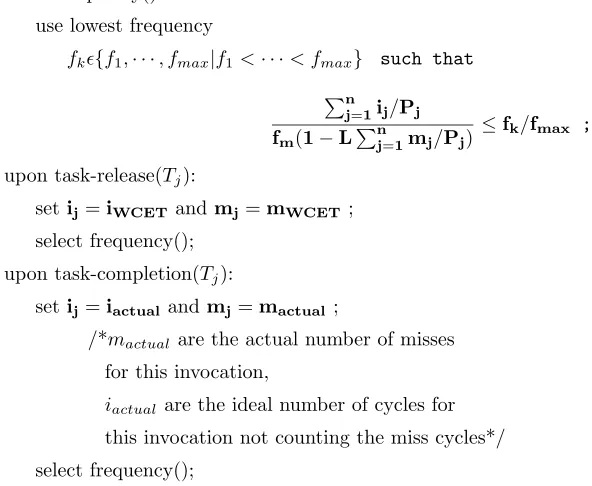
Figure 5.2: FAST-Cycle conserving DVS for EDF

5.3 FAST - Cycle-Conserving RT-DVS

The cycle conserving RT-DVS by Pillai and Shin [27] calculates the utilization for a task set at every task release and task completion. Upon task release, the utilization is calculated based on the WCET. Upon task completion, the utilization is calculated by considering the actual execution time of the completed task instead of the WCET. This algorithm uses the static slack available in the system as well as the dynamic slack generated due to early task completions. Figure 5.2 shows the necessary modifications to the original algorithm to incorporate the FAST equations.

(30)

5.5 and 5.6.

5.4 FAST - Look-Ahead RT-DVS

(31)

select-frequency(x): use lowest frequency

fk²{f1,· · ·, fmax|f1<· · ·< fmax}

such thatx≤fk/fmax;

upon task-release(Tj):

setc lef tj=Cj,

i leftj=i wcetj andm leftj=m wcetj ;

defer();

upon task-completion(Tj):

setc lef tj=Cj,

i leftj=i wcetj andm leftj=m wcetj ;

defer();

during task-execution(Tj):

decrementc lef tj,i leftj andm leftj ;

defer():

setU =C1/P1+· · ·+Cn/Pn;

sets= 0 ;

fori= 1 to n,Tj ² T1,· · ·, Tn|D1≥ · · · ≥Dn

/*Note: reverse EDF order of tasks*/

setU =U−Cj/Pj ;

setxj= max(0, c lef tj−(1−U)(Dj−Dn)) ;

setU =U+ (c lef tj−xj)/(Dj−Dn) ;

sets=s+xj; s=s−xn;

t=Dn−current time;

x= (i leftn+s)/t

fm(1−L×m leftn/t) ;

select-frequency(x);

(32)

Chapter 6

Validation Experiments

This chapter describes the experiments performed to verify the FAST analysis tool and the FAST-DVS schemes. Six real-time benchmarks from the C-lab real-time benchmark suite [9], namely srt, fft, mm, lms, adpcm and cnt, are used to calculate the WCET and create the tasksets for all the experiments.

6.1 Testing the FAST Analysis tool

To test the FAST framework, the FAST analysis tool is compared with the tra-ditional static timing analysis tool. The tratra-ditional static timing analyzer provides a tight bound of the execution time for the application. It is expected that the WCET calculated by the FAST analysis tool will match the WCET obtained from the traditional static timing analyzer.

6.1.1 Traditional Static Timing Analysis Tool

(33)

latency of 100ns is used. The timing analyzer takes into account a 8KB I-cache and a 8KB D-cache.

Real-time applications are compiled into assembly code using the GCC PISA-compiler. The control-flow information is supplied to the static instruction cache simulator to obtain the caching categorizations for real-time application. These categorizations ob-tained for the I-cache are used in the timing analyzer to determine accurate WCET. Since an accurate static D-cache simulator is unavailable at this time, categorizations for the data accesses are obtained by assuming that a constant number of data cache accesses are misses for each application to model compulsory misses. The remaining references are considered to be hits, which models a sufficiently large cache. This assumption mimics a data cache simulator. The WCET calculated is an upper-bound for the real-time application but is not a tight bound. Using these data cache categorizations is better than assuming that all data accesses are misses.

6.1.2 FAST Analysis Tool

The traditional static timing analyzer was redesigned to create the FAST frame-work. The FAST analysis tool, like its predecessor, is based on the portable ISA (PISA) used by the architectural simulator. The FAST tool uses the same six-stage simple in-order pipeline used in the traditional static timing analysis tool. The static cache simulation strategy and the static data cache assumption remain the same as well. The simplifying assumption used for data accesses does not affect the design of FAST, i.e., the frequency model supports a more precise static data cache analysis as well.

The traditional static analysis tool calculates the WCEC for the application with-out differentiating between cycles contributed by memory accesses and cycles contributed by processor operations. The static timing analyzer is converted into the FAST analysis tool by changing the method of calculating WCEC; by separating the cycles contributed by the memory and those contributed by the processor.

(34)

the two equations by using another first-order polynomial equation providing a safe upper bound. The new first-order polynomial is formed by using the maximum values obtained at minimum frequency (100MHz) and maximum frequency (1GHz) from the two conflicting first-order equations. This may result in slight overestimations but, overall, still provides a sufficiently tight bound of the WCEC, as will be seen. The branch misprediction penalty is removed from the FAST equation if branch misprediction overlaps with a data miss stall. The overestimation caused by instructions with execution latencies higher than one are not removed from the equation as they contribute insignificant savings.

The procedure of obtaining WCET estimates from the FAST analysis tool remains the same as the procedure for the traditional static timing analyzer, explained in section 6.1.1.

6.1.3 Experiment 1: Accuracy of FAST analysis tool

Six real-time benchmarks from the C-lab real-time benchmark suite [9], commonly utilized for WCET experiments, are studied. Three floating-point benchmarks, adpcm, lms and fft, as well as three integer benchmarks, cnt, srt and mm, are analyzed. These benchmarks were compiled by the PISA GCC compiler integrated with the SimpleScalar-based tool set. From the compilation of these benchmarks, the control-flow graphs and instruction layouts were obtained, which are taken as inputs to the FAST analyzer and the

Bench- Equations WCET:Static timing analysis/ FAST (WCEC)

marks i m 100MHZ 400MHZ 700MHZ 1000MHZ

fft 355933 24658 600628/ 1340578/ 2079876/ 2820478/ 602675 1342625 2081993 2822525 adpcm 3026370 544104 8433905/ 24749525/ 41065145/ 57380765/

8467410 24790530 41113650 57436770 lms 167890 29905 466438/ 1363598/ 2260748/ 3157898/ 466940 1364090 2261240 3158390 cnt 71221 6066 131880/ 313860/ 495840/ 677820/ 131881 313861 495841 677821 mm 2038538 59134 2629877/ 4403897/ 6177917/ 7951937/

2629878 4403898 6177918 7951938 srt 3509420 102145 4530868/ 7595218/ 10659568/ 13723918/

4530870 7595220 10659570 13723920

(35)

static cache analyzer. The FAST output is the WCEC in the form of a parametric equation conforming with the parametric frequency model. The same benchmarks were also exposed to the original static timing analysis tool set for comparison. The original static timing analyzer must be run separately for each frequency under consideration to account for changed memory latency for a given processor frequency. In contrast, the FAST framework captures the same effect in an equation (derived from a single analysis step).

6.1.4 Results for FAST Analysis Tool

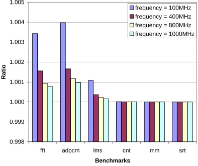
The WCEC equations for the six benchmarks obtained from the static timing analysis tool and the FAST tool are compiled in Table 6.1 and in Figure 6.1.

The FAST scheme differs from conventional static timing analysis without para-metric expressions of frequencies by less than half a percent. Hence, it is concluded that

0.998 0.999 1.000 1.001 1.002 1.003 1.004 1.005

fft adpcm lms cnt mm srt

Benchmarks

R

a

ti

o

frequency = 100MHz

frequency = 400MHz

frequency = 800MHz

frequency = 1000MHz

(36)

the FAST equations accurately model the WCEC obtained from the static analysis tool. Since the effects of scaling on WCEC are accurately modeled by the FAST equations, the scaling of the WCET can also be accurately captured.

Table 6.1 shows the WCEC for all six benchmarks calculated for four different fre-quencies using the FAST equations and compared with the corresponding WCEC obtained from the static timing analysis tool. Figure 6.1 plots the ratio of the WCET for the FAST tool and the static timing analysis tool.

As shown in the Table 6.1 and Figure 6.1, cnt, mm and srt show that the FAST bounds on WCET match the bounds obtained by the static timing analyzer exactly. For fft, adpcm and lms the FAST bounds on WCET are very close to the bounds obtained by the static timing analyzer. The overestimation in these benchmarks is due to the presence of floating point operations that have overlapping execution latencies with memory stalls (see Section 2.2, Figure 3.4).

Thus, the FAST tool can accurately model the WCEC of tasks with a negligible error (<1%) by using the parametric frequency model.

6.2 Testing FAST-DVS Schemes

The performance of the FAST-DVS schemes developed in the previous chapter is compared to the original DVS schemes [27]. The FAST-DVS schemes are expected to use the leverage provided by the FAST equations to outperform the original DVS schemes.

6.2.1 DVS Real-Time Scheduling Algorithms

(37)

6.2.2 Power Modeling

Two power models are employed to evaluate the performance of the scheduling algorithms - the generic power model and the Wattch power model.

1. The generic power model assumes that power consumed in each cycle depends only on the frequency and voltage of operation. The hardware structures accessed in the cycle are ignored. The power is calculated usingP ower=V oltage2

×f requency.

2. The Wattch power models [6] are integrated into the architectural simulator to mea-sure power and energy. The original Wattch models use a Reservation Update Unit (RUU) based microarchitecture. The models are modified to closely match the struc-tures of a simple processor. Modifications to support dynamic voltage scaling (DVS) were also made.

The frequency/voltage settings used for DVS are loosely based on the Intel Xscale, which is reported to have 5 settings ranging from 150 MHz/0.76 V to 1 GHz/1.8 V [18]. From the Xscale, 37 frequency/voltage settings were extrapolated, ranging from 100 MHz/0.70 V to 1 GHz/1.8 V in 25 MHz/0.03 V increments.

6.2.3 Simulator 1: Event-Based DVS Simulator

(38)

in the SimpleScalar-based simulator [28]. By exploiting a cycle-accurate architectural sim-ulator, the total number of cache misses as well as the total number of cycles executed can be obtained. The execution times obtained from the architectural simulator are scaled with frequency using the same assumption used while formulating the FAST parametric model. Namely, it is assumed that the total number of execution cycles does not remain constant with frequency. The same execution time scaling method is used for all the voltage scaling algorithms.

To evaluate the different FAST-DVS and DVS schemes, several tasksets were formed using the cnt, srt, mm, adpcm, fft and lms benchmarks. Three groups were formed as follows - G1: cnt, srt, mm (all integer), G2:adpcm, fft, lms (all floating point) and G3:cnt, mm, fft, lms (mixed). The periods were chosen for each benchmark and from each group two tasksets are created – one with high utilization, and one with low utilization. The high utilization tasksets have a utilization of approximately 0.9 while the low utilization tasksets have a utilization of approximately 0.5.

The energy per cycle is calculated at a particular frequency by using the relation Energy=V oltage2

×f requency. This simulator only implements the generic power model.

6.2.4 Simulator 2: Architectural Simulator

A multi-tasking environment has been modeled using a cycle-accurate simulator built using the SimpleScalar toolset [7]. The architectural simulator supports a simple six-stage in-order processor pipeline model.

The simulator models various memory-mapped counters (e.g., the watchdog counter) and registers (e.g., the current frequency register, etc.). The scheduler accesses these regis-ters and counregis-ters to specify the next task, the next event, etc.

The benchmarks and scheduler are compiled using the SimpleScalar GCC-based compiler which targets the SimpleScalar ISA (PISA), a MIPS-like ISA [7]. Thus, actual binaries are loaded and executed by the processor simulator. Each task has its own binary, including the scheduler itself.

Currently, the simulator has the ability to execute up to four independent threads, one of which is the real-time scheduler itself. The scheduler thread is invoked on two events: (1) completion of a task and (2) release of a task.

(39)

by the processor, called the release timer. Before turning the processor over to the next task, the scheduler sets the release timer to interrupt at the next task release.

At the start of simulation, the scheduler is invoked first. After deciding which task to execute next, the scheduler sets the release timer and is swapped out. The next task is then swapped in. The scheduler is invoked again when either the task finishes or is interrupted by the release timer. The scheduler makes a scheduling decision on each invocation.

In summary, the software and hardware of the multi-tasking system are modeled in significant detail. In particular, the scheduler overhead, both in terms of processor cycles and power consumption, is included by virtue of executing it like any other task. The simulator uses the generic power model, as well as the Wattch power model.

6.2.5 Experiment 2a: Performance of FAST-DVS schemes with the Event-Based Simulator

To evaluate the different FAST-DVS and DVS schemes, several tasksets were formed using the cnt, srt, mm, adpcm, fft and lms benchmarks. Three groups were formed as follows - G1: cnt, srt, mm (all integer), G2:adpcm, fft, lms (all floating point) and G3:cnt, mm, fft, lms (mixed). Periods were chosen for each benchmark, and from each group two tasksets are created – one with high utilization, and one with low utilization. The high utilization tasksets have a utilization of approximately 0.9 while the low utilization tasksets have a utilization of approximately 0.5.

The tasksets were executed on Simulator 1 (event-based simulator) using the dif-ferent scheduling algorithms. The power consumed by the tasksets for each scheduling algorithm were noted.

(40)

For the integer taskset G1, savings are considerable (excess of 50%) between the original scheme and the corresponding FAST scheme for the static and cycle-conserving approaches (Figures 6.2(a) and 6.2(b)). The look-ahead scheme shows none or only marginal savings under FAST for high and lower utilizations, respectively. This is caused by fact that the FAST look-ahead scheme runs the taskset at a lower frequency and has to recover by raising the frequency more often than the original look-ahead scheme.

The results are also sensitive to the task set, as a comparison with the floating-point taskset G2 shows. Figures 6.2(c) and 6.2(d) indicate that G2 still experiences considerable savings for high utilizations – and slightly lower ones for lower utilizations – under the corresponding FAST scheme. In case of G2, savings for the static and cycle-conserving schemes are even higher. The results for the integer/floating point mix of G3 in Figures 6.2(e) and 6.2(f) show savings at levels between the G1 and G2 tasksets for static and cycle-conserving schemes. The look-ahead version of FAST results in less significant savings, mostly due to already very aggressive savings due to the original look-ahead scheme.

All results depend on the FAST equation for the benchmarks. The scalability of the WCET depends on the number of misses counted during timing analysis. Due to a worst-case analysis, the number of misses are usually highly exaggerated, especially for data caches. This means that the original schemes are penalized heavily due to their assumptions about scaling the WCET. Using the FAST equations, the DVS schemes can improve the tightness of the WCET, which is already highly exaggerated, thereby improving energy consumption.

(41)

6.2.7 Experiment 2b: Performance of FAST-DVS schemes with the Ar-chitectural Simulator

The tasksets used for this experiment are the same as those described in section 6.2.5. The three tasksets G1, G2 and G3 with a high and a low utilization were executed on Simulator 2 (architectural simulator) using the different scheduling algorithms. The power consumed by the tasksets for each scheduling algorithm were noted.

6.2.8 Results for FAST-DVS Schemes with the Architectural Simulator Figures 6.3(a) to 6.3(f) show the Energy for all the DVS schemes normalized to the base EDF scheme for all six tasksets. The figures show a decrease in power consumption for all the FAST-DVS schemes when compared to the original RT-DVS schemes. Note that the generic energy model and the Wattch power model are used to obtain results.The first, third and fifth set of bars in the graphs show the energy consumption for the original RT-DVS schemes. The second, fourth and sixth bars in the graphs show the improved energy consumption for the FAST-DVS schemes.

The results obtained differ from those from the Event-Based Simulator but show a similar trend. The Normalized values for energy are higher, but the difference between the performance of the original and the FAST schemes is promising.

The difference between the original and FAST version of the static scheme is between 30% to 55%. The normalized values for the generic energy model and the Wattch model are different, but show a similar trend of energy savings.

The original cycle conserving scheme is an aggressive dynamic scheme. The FAST cycle conserving scheme improves the original scheme by providing extra savings between 16% to 38%.

The look-ahead scheme is the most aggressive RT-DVS scheme and the energy savings observed are between -4% and 9%. It must be noted that usually, the FAST look-ahead scheme runs at a lower frequency, but due to the aggressive nature of the algorithm, it has to recover at a higher frequency as compared to the original scheme. Due to the quadratic nature of the Energy-frequency relation.

(42)

(43)

0 0.05 0.1 0.15 0.2 0.25 0.3 0.35 Static RT-DVS FAST Static RT-DVS Cycle Conserving RT-DVS FAST Cycle Conserving RT-DVS Look-ahead RT-DVS FAST Look-ahead RT-DVS DVS-EDF Schemes E n e rg y n o rm a li z e d t o b a s e E D F

(a) Taskset G1 with utilization 0.9

0 0.02 0.04 0.06 0.08 0.1 0.12 Static RT-DVS FAST Static RT-DVS Cycle Conserving RT-DVS FAST Cycle Conserving RT-DVS Look-ahead RT-DVS FAST Look-ahead RT-DVS DVS-EDF Schemes E n e rg y n o rm a li z e d t o b a s e E D F

(b) Taskset G1 with utilization 0.5

(c) Taskset G2 with utilization 0.9

0 0.02 0.04 0.06 0.08 0.1 0.12 0.14 0.16 0.18 Static RT-DVS FAST Static RT-DVS Cycle Conserving RT-DVS FAST Cycle Conserving RT-DVS Look-ahead RT-DVS FAST Look-ahead RT-DVS DVS-EDF Schemes E n e rg y n o rm a li z e d t o b a s e E D F

(d) Taskset G2 with utilization 0.5

0 0.05 0.1 0.15 0.2 0.25 0.3 0.35 0.4 Static RT-DVS FAST Static RT-DVS Cycle Conserving RT-DVS FAST Cycle Conserving RT-DVS Look-ahead RT-DVS FAST Look-ahead RT-DVS DVS-EDF Schemes E n e rg y n o rm a li z e d t o b a s e E D F

(e) Taskset G3 with utilization 0.9

(f) Taskset G3 with utilization 0.5

(44)

(a) Taskset G1 with utilization 0.9 (b) Taskset G1 with utilization 0.5

(c) Taskset G2 with utilization 0.9 (d) Taskset G2 with utilization 0.5

(e) Taskset G3 with utilization 0.9 (f) Taskset G3 with utilization 0.5

(45)

Chapter 7

Related Work

This chapter describes prior work in timing analysis for real-time applications and DVS scheduling algorithms.

Recently, a number of research groups have addressed various issues in the area of predicting the worst-case execution time (WCET) of real-time programs. Conventional methods for static analysis have been extended from unoptimized programs on simple CISC processors to optimized programs on pipelined RISC processors, and from uncached archi-tectures to instruction and data caches [26, 21, 16, 25, 33, 20]. All these methods obtain discrete values to bound the WCET in a non-parametric fashion.

Vivancos et al. describe techniques for addressing static timing analysis for vari-able loop bounds [31]. The so-called parametric timing analysis allows dynamic schedulers to re-assess the WCET based on dynamically determined loop bounds during program exe-cution. Chapmanet al. [11] used path expressions to combine a source-oriented parametric approach of WCET analysis with timing annotations, verifying the latter through the for-mer. Bernat and Burns also proposed using algebraic expressions to represent the WCET of subprograms, where the algebraic expression is parameterized by some of the subprogram’s parameters [5]. These approaches differ in that they address fundamental problems in static timing analysis. The FAST approach, in contrast, aims at isolating execution effects as a function of the processor frequency, a unique, unprecedented approach complementing existing work on static timing analysis.

(46)

Chapter 8

Conclusions and Future Work

(47)

Bibliography

[1] A. Anantaraman, K. Seth, K. Patil, E. Rotenberg, and F. Mueller. Virtual simple architecture (VISA): Exceeding the complexity limit in safe real-time systems. In

International Symposium on Computer Architecture, pages 250–261, June 2003.

[2] R. Arnold, F. Mueller, D. B. Whalley, and M. Harmon. Bounding worst-case instruction cache performance. InIEEE Real-Time Systems Symposium, pages 172–181, December 1994.

[3] H. Aydin, R. Melhem, D. Mosse, and P. Mejia-Alvarez. Dynamic and agressive schedul-ing techniques for power-aware real-time systems. In IEEE Real-Time Systems

Sym-posium, December 2001.

[4] M. E. Benitez and J. W. Davidson. A portable global optimizer and linker. In ACM

SIGPLAN Conference on Programming Language Design and Implementation, pages

329–338, June 1988.

[5] G. Bernat and A. Burns. An approach to symbolic worst-case execution time analysis.

In25th IFAC Workshop on Real-Time Programming, May 2000.

[6] David Brooks, Vivek Tiwari, and Margaret Martonosi. Wattch: A framework for architectural-level power analysis and optimizations. InProceedings of the 27th Annual

International Symposium on Computer Architecture, pages 83–94, Vancouver, British

Columbia, June 2000. IEEE Computer Society and ACM SIGARCH.

[7] Doug Burger, Todd M. Austin, and Steve Bennett. Evaluating future microprocessors: The simplescalar tool set. Technical Report CS-TR-1996-1308, University of Wisconsin, Madison, July 1996.

(48)

[9] C-Lab. Wcet benchmarks. Available from http://www.c-lab.de/home/en/download.html.

[10] A.P. Chandrakasan, S. Sheng, and R. W. Brodersen. Low-power cmos digital design.

InIEEE Journal of Solid-State Circuits, Vol. 27, pp. 473-484., April, 1992.

[11] R. Chapman, A. Burns, and A. Wellings. Combining static worst-case timing analysis and program proof. Real-Time Systems, 11(2):145–171, 1996.

[12] H. Chetto and M. Chetto. Some results of the earliest deadline scheduling algorithm.

IEEE Transactions on Software Engineering, 15(10):1261–1269, October 1989.

[13] A. Dudani, F. Mueller, and Y. Zhu. Energy-conserving feedback edf scheduling for embedded systems with real-time constraints. In ACM SIGPLAN Joint Conference Languages, Compilers, and Tools for Embedded Systems (LCTES’02) and Software

and Compilers for Embedded Systems (SCOPES’02), pages 213–222, June 2002.

[14] F. Gruian. Hard real-time scheduling for low energy using stochastic data and dvs processors. In Proceedings of the International Symposium on Low-Power Electronics

and Design ISLPED’01, Aug 2001.

[15] C. A. Healy, R. D. Arnold, F. Mueller, D. Whalley, and M. G. Harmon. Bound-ing pipeline and instruction cache performance. IEEE Transactions on Computers, 48(1):53–70, January 1999.

[16] C. A. Healy, D. B. Whalley, and M. G. Harmon. Integrating the timing analysis of pipelining and instruction caching. In IEEE Real-Time Systems Symposium, pages 288–297, December 1995.

[17] Y. Hur, Y. H. Bae, S.-S. Lim, B.-D. Rhee, S. L. Min, C. Y. Park, M. Lee, H. Shin, and C. S. Kim. Worst case timing analysis of RISC processors: R3000/R3010 case study.

InIEEE Real-Time Systems Symposium, pages 308–319, December 1995.

[18] Intel. Intel XScale Microarchitecture Technical Summary, July 2000.

(49)

[20] Y.-T. S. Li, S. Malik, and A. Wolfe. Cache modeling for real-time software: Beyond direct mapped instruction caches. InIEEE Real-Time Systems Symposium, pages 254– 263, December 1996.

[21] S.-S. Lim, Y. H. Bae, G. T. Jang, B.-D. Rhee, S. L. Min, C. Y. Park, H. Shin, and C. S. Kim. An accurate worst case timing analysis for RISC processors. InIEEE Real-Time

Systems Symposium, pages 97–108, December 1994.

[22] C. Liu and J. Layland. Scheduling algorithms for multiprogramming in a hard-real-time environment. J. of the Association for Computing Machinery, 20(1):46–61, January 1973.

[23] T. Lundqvist and P. Stenstr¨om. An integrated path and timing analysis method based on cycle-level symbolic execution. Real-Time Systems, 17(2/3):183–208, November 1999.

[24] D. Mosse, H. Aydin, B. Childers, and R. Melhem. Compiler-assisted dynamic power-aware scheduling for real-time applications. InWorkshop on Compilers and Operating

Systems for Low Power, October 2000.

[25] F. Mueller. Timing analysis for instruction caches. Real-Time Systems, 18(2/3):209– 239, May 2000.

[26] C. Y. Park. Predicting program execution times by analyzing static and dynamic program paths. Real-Time Systems, 5(1):31–61, March 1993.

[27] P. Pillai and K. Shin. Real-time dynamic voltage scaling for low-power embedded operating systems. InSymposium on Operating Systems Principles, 2001.

[28] E. Rotenberg. Using variable-Mhz microprocessors to efficiently handle uncertainty in real-time systems. In 34th International Symposium on Microarchitecture, pages 28 – 39, December 2001.

[29] J. Stankovic, M. Spuri, K. Ramamritham, and G. Buttazzo. Deadline Scheduling for

Real-Time Systems. Kluwer, 1998.

[30] H. Theiling and C. Ferdinand. Combining abstract interpretation and ilp for mi-croarchitecture modelling and program path analysis. In IEEE Real-Time Systems

(50)

[31] E. Vivancos, C. Healy, F. Mueller, and D. Whalley. Parametric timing analysis. In

ACM SIGPLAN Workshop on Language, Compiler, and Tool Support for Embedded

Systems, August 2001.

[32] J. Wegener and F. Mueller. A comparison of static analysis and evolutionary testing for the verification of timing constraints.Real-Time Systems, 21(3):241–268, November 2001.

(51)

(52)

APPENDIX

Modified Look-ahead DVS-EDF

A number of DVS schemes were proposed by Pillai and Shin for scheduling hard real-time systems [27]. A simple, static scaling version uniformly scales the frequency for all tasks based on utilization tests for schedulability, both for rate-monotone and EDF scheduling. Cycle-conserving EDF lowers utilization upon task completion temporarily to the proportion of the actual execution time. Look-ahead EDF is an extension to these scheme that capitalizes on early task completion by deferring work for future tasks in favor of scaling the current task. Scaling of the current task occurs based on a modified utilization test that benefits from both idle slots and early task completion. At any completion (both early and on time), the utilization is effectively reduced for the completing task (up until its next release time).

Specifically, upon task completion,cci =c lef t1= 0 according to Cycle-Conserving EDF and Look-ahead EDF, respectively. The defer calculations of Look-ahead EDF then reassesses the utilization based on future and past deadlines for released and completed tasks, respectively.

(53)

Frequency-aware Static Timing Analysis for Power-aware Embedded Architectures

Contents

List of Figures

Chapter 1

Introduction

1.1

Worst-Case Execution Time

1.2

Dynamic Voltage Scaling

1.3

Parametric Frequency Model

1.4

Outline

Chapter 2

Effects of frequency scaling on

WCET

Frequency (MHz)

N

u

m

b

e

r

o

f

C

y

c

le

s

Frequency (MHz)

T

im

e

(

m

s

)

Chapter 3

Parametric Frequency Model

A:

add R2, R1, R3

B:

load R4, [M1]

C:

add R2, R1, R4

D:

add R2, R1, R5

Cycles

IF

ID

IS

EX

MEM

WB

2

3

4

5

1

6

A

A

A

A

A

A

B

B

B

B

C

D

C

D

C

D

C

B

B C