Abstract
WOOLARD, RYAN. Logistical Model for Closed Loop Recycling of Textile Materials. (Under the direction of Dr. Jeff Joines and Dr. Kristin Thoney.)
In the United States alone, people consume and discard over 500 billion pounds of wastes annually. Wastes discarded in landfills create threats to land, air, and water, but also represent lost resources. Recycling has the ability to divert wastes from landfills and recover precious raw materials. However, recycling activities are only as efficient as the reverse logistics and supply chains that support them. These areas are relatively new, but successful implementations have real benefits for companies in terms of profits and environmental goodwill. Many companies are creating closed loop supply chains where forward and reverse activities are interlinked in cyclical processes. Ideally, a virgin input enters the system only once and is recycled forever. The problem with most current closed loop supply chains is that they are product-specific. When a closed-loop supply chain is designed, the product must be designed so that it can easily be recycled back into the supply chain. The problem is that the product must contain a minimum number of dissimilar components. For textile products, this presents a real challenge because of fiber blends and finishes that make component separation difficult. These problems create the need to design textile recycling systems.
This research focuses on the logistical systems necessary to recycle textile materials. Methodologies for estimating post-consumer carpet (PCC) returns and trailer loading
Logistical Model for Closed Loop Recycling of Textile Materials
by Ryan Woolard
A thesis submitted to the Graduate Faculty of North Carolina State University
in partial fulfillment of the requirements for the degree of
Master of Science
Textile Engineering
Raleigh, North Carolina 2009
APPROVED BY:
_______________________________ ______________________________
Dr. Jeff Joines Dr. Kristin Thoney
Chair Advisory Committee Co-Chair Advisory Committee
________________________________ ______________________________
Dr. Russell E. King Dr. W. Gilbert O’Neal
Biography
Ryan Woolard grew up in Belhaven, North Carolina. He graduated with a Bachelor of Science degree in Industrial and Systems Engineering from North Carolina State
University in the fall of 2005. During the summer of 2004, he interned with DEL
Laboratories, Inc. where he worked closely with the Industrial Engineering department to improve packaging efficiency and line performance. Ryan participated in Milliken &
Acknowledgements
I would like extend thanks to my committee, Dr. Jeff Joines, Dr. Kristin Thoney, and Dr. Russell King for all of their advice and guidance in the completion of my research. I would especially like to express my appreciation to Mike Bucci, who spent hours
Table of Contents
List of Figures ... vi
List of Tables ... xi
List of Equations ... xiii
1 Introduction ... 1
1.1 Background ... 1
1.2 Specific Research Objectives ... 3
1.3 Research Outline ... 4
2 Literature Review... 5
2.1 History of Reverse Logistics ... 5
2.2 Modern Principles of Reverse Logistics ... 7
2.2.1 Why Reverse Logistics Matters ... 7
2.2.2 How Reverse Logistics Works... 12
2.3 Forward and Reverse Supply Chains ... 15
2.3.1 Feedback Mechanisms in Reverse Supply Chains ... 17
2.3.2 Business Models ... 21
2.3.3 What Makes Closed Loop Supply Chains Difficult ... 22
2.4 Recycling of Textile Materials... 24
2.4.1 Apparel Reverse Networks ... 24
2.4.2 Carpet Primer ... 28
2.4.3 Carpet Recycling History ... 31
2.4.4 Carpet Reverse Network ... 33
2.4.4.1 Carpet Waste Forecasts and Collections ... 34
2.4.4.2 Carpet Collection Sites ... 41
2.4.4.3 Carpet Recycling Sites ... 43
2.4.4.4 Reclaimed Carpet Materials ... 45
2.4.4.5 Previous Carpet Recycling Mathematical Models ... 47
2.5 Proceeding Research ... 48
3 Carpet Reverse Networks ... 50
3.1 Carpet Network Flow Diagram ... 50
3.2 Carpet Recycling Site Location Allocation Models ... 52
3.2.1 Model Description ... 53
3.2.2 Calculation of Annual PCC Truckloads ... 55
3.2.3 Assignment of Annual PCC Weight Percentages to Collection Sites ... 58
3.2.4 CARE PCC Reverse Network Models ... 64
3.2.4.1 Overlapping Collection Radii ... 64
3.2.4.2 Non-Overlapping Collection Radii ... 71
3.2.5 National PCC Reverse Models with Economies of Scale ... 81
3.2.5.1 Original and Adjusted Economies of Scale Curves ... 86
3.2.5.2 Adjusted Economies of Scale Curve ... 92
4 Carpet Reverse Supply Chain Cost Model ... 102
4.2 Transportation Costs ... 104
4.3 Recycling Sites... 107
4.4 Reverse Supply Chain ... 109
5 Conclusions ... 116
6 Recommendations for Future Work... 120
6.1 Fixed Sites in the Location Allocation Model ... 120
6.2 Capacitated PCC National Network Location Allocation Model ... 121
6.3 Apparel Reverse Networks ... 125
6.3.1 Garment Network Flow Diagram ... 127
6.3.2 Garment Recycling Network ... 128
7 References ... 132
8 Appendices ... 138
A CARE Reclamation Centers ... 139
B CARE Collection Site Distance Matrix ... 140
C CARE Model Results - Non-Overlapping Collection Radii ... 141
D Estimated Shipping Rates ... 151
E National Network Model - Original and Adjusted Economies of Scale ... 155
F National Network Model - Adjusted and No Economies of Scale ... 157
G Post-Consumer Carpet (PCC) Cost Models ... 182
List of Figures
Figure 2-1: Reverse Logistics Hierarchy (modified from Dhanda and Peters, 2008) ... 11
Figure 2-2: Reverse Logistics Processes... 15
Figure 2-3: Generic Reverse Supply Chain ... 16
Figure 2-4: Generic Closed Loop Supply Chain... 17
Figure 2-5: Pyramid Model for Textile Recycling Categories by Quantity ... 28
Figure 2-6: Typical Carpet Construction ... 29
Figure 2-7: Component Mass/Area for a Typical Carpet (g/m2) ... 29
Figure 2-8: Task Network for Carpet Recycling ... 34
Figure 2-9: Annual Estimated Carpet Discard Weight ... 36
Figure 2-10: CARE Collection Center Locations ... 40
Figure 2-11: Breakdown of Diversion by Types of Companies ... 40
Figure 2-12: CARE Annual Landfill Diversion Weights ... 41
Figure 2-13: Distribution of Carpet Fiber Handled ... 42
Figure 3-1: Carpet Network Flow Diagram ... 51
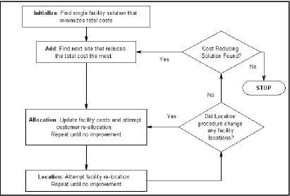
Figure 3-2: Model Logic Flow Diagram ... 55
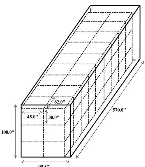
Figure 3-3: Optimized Freight Trailer Loading ... 57
Figure 3-4: Collection Network Diagram ... 60
Figure 3-5: National Collection Network ... 63
Figure 3-6: 1 Site - First Site Optimal (23.82 mi. Overlapping Radii) ... 67
Figure 3-7: 1 Site - First Site NC/SC/GA (23.82 mi. Overlapping Radii)... 67
Figure 3-8: 2 Sites - First Site Optimal (23.82 mi. Overlapping Radii) ... 67
Figure 3-9: 2 Sites - First Site NC/SC/GA (23.82 mi. Overlapping Radii) ... 67
Figure 3-10: 3 Sites - First Site Optimal (23.82 mi. Overlapping Radii) ... 68
Figure 3-11: 3 Sites - First Site NC/SC/GA (23.82 mi. Overlapping Radii) ... 68
Figure 3-12: 1 Site - First Site Optimal (Regional Tip Fee Overlapping Radii) ... 70
Figure 3-13: 1 Site - First Site NC/SC/GA (Regional Tip Fee Overlapping Radii) ... 70
Figure 3-14: 2 Sites - First Site Optimal (Regional Tip Fee Overlapping Radii) ... 70
Figure 3-15: 2 Sites - First Site NC/SC/GA (Regional Tip Fee Overlapping Radii) ... 70
Figure 3-16: 3 Sites - First Site Optimal (Regional Tip Fee Overlapping Radii) ... 70
Figure 3-17: 3 Sites - First Site NC/SC/GA (Regional Tip Fee Overlapping Radii) ... 70
Figure 3-18: United States Population Density Map ... 71
Figure 3-19: % Change of Weights from Overlapping to Non-Overlapping Radii ... 74
Figure 3-20: Weights for Collection Sites with Varying Radii ... 75
Figure 3-21: CARE Network Transportation Costs... 77
Figure 3-22: 6 Sites - First Site Optimal (11.91 mi. Non-Overlapping Radii) ... 80
Figure 3-23: 6 Sites - First Site NC/SC/GA (11.91 mi. Non-Overlapping Radii) ... 80
Figure 3-24: 6 Sites - First Site Optimal (23.82 mi. Non-Overlapping Radii) ... 80
Figure 3-25: 6 Sites - First Site NC/SC/GA (23.82 mi. Non-Overlapping Radii) ... 80
Figure 3-26: 6 Sites - First Site Optimal (47.64 mi. Non-Overlapping Radii) ... 80
Figure 3-27: 6 Sites - First Site NC/SC/GA (47.64 mi. Non-Overlapping Radii) ... 80
Figure 3-28: Estimated Shipping Rates and Diesel Fuel Costs ... 85
Figure 3-30: Economies of Scale Curve (Original) ... 88
Figure 3-31: Economies of Scale Curve (Adjusted) ... 88
Figure 3-32: 4 Sites - 1,800 Million Lbs. (Original Economies of Scale Curve) ... 90
Figure 3-33: 4 Sites - 1,800 Million Lbs. (Adjusted Economies of Scale Curve) ... 90
Figure 3-34: Adjusted Economies of Scale Curve and No Economies of Scale ... 92
Figure 3-35: National Network Transportation Costs (Adjusted Economies of Scale Curve) 96 Figure 3-36: National Network Transportation Costs (No Economies of Scale) ... 96
Figure 3-37: National Network Recycling Processing Costs (Adjusted Economies of Scale Curve) ... 96
Figure 3-38: National Network Recycling Processing Costs (No Economies of Scale) ... 96
Figure 3-39: National Network Total Costs (Adjusted Economies of Scale Curve) ... 97
Figure 3-40: National Network Total Costs (No Economies of Scale) ... 97
Figure 3-41: 5 Sites - 300 Million Lbs. (Adjusted Economies of Scale Curve) ... 99
Figure 3-42: 5 Sites - 300 Million Lbs. (No Economies of Scale) ... 99
Figure 3-43: 5 Sites - 600 Million Lbs. (Adjusted Economies of Scale Curve) ... 99
Figure 3-44: 5 Sites - 600 Million Lbs. (No Economies of Scale) ... 99
Figure 3-45: 5 Sites - 1,200 Million Lbs. (Adjusted Economies of Scale Curve) ... 99
Figure 3-46: 5 Sites - 1,200 Million Lbs. (No Economies of Scale) ... 99
Figure 3-47: 5 Sites - 1,800 Million Lbs. (Adjusted Economies of Scale Curve) ... 100
Figure 3-48: 5 Sites - 1,800 Million Lbs. (No Economies of Scale) ... 100
Figure 3-49: 5 Sites - 2,400 Million Lbs. (Adjusted Economies of Scale Curve) ... 100
Figure 3-50: 5 Sites - 2,400 Million Lbs. (No Economies of Scale) ... 100
Figure 6-1: Diseconomies of Scale Curve ... 122
Figure 6-2: 1 Site - 1,800 Million Lbs. (Diseconomies of Scale Curve) ... 124
Figure 6-3: 2 Sites - 1,800 Million Lbs. (Diseconomies of Scale Curve) ... 124
Figure 6-4: 3 Sites - 1,800 Million Lbs. (Diseconomies of Scale Curve) ... 124
Figure 6-5: 4 Sites - 1,800 Million Lbs. (Diseconomies of Scale Curve) ... 124
Figure 6-6: 5 Sites - 1,800 Million Lbs. (Diseconomies of Scale Curve) ... 124
Figure 6-7: 6 Sites - 1,800 Million Lbs. (Diseconomies of Scale Curve) ... 124
Figure 6-8: Apparel Network Flow Diagram... 125
Figure 6-9: Garment Network Flow Diagram ... 127
Figure 6-10: Continental United States Laundry Locations ... 128
Figure 6-11: 1 Site - 13 Million Lbs. ... 131
Figure 6-12: 2 Sites - 13 Million Lbs... 131
Figure 6-13: 3 Sites - 13 Million Lbs... 131
Figure 6-14: 4 Sites - 13 Million Lbs... 131
Figure 6-15: 5 Sites – 13 Million Lbs. ... 131
Figure 6-16: 6 Sites - 13 Million Lbs... 131
Figure 8-1: % Change in Transportation Costs between Sites ... 142
Figure 8-2: 1 Site - First Site Optimal (11.91 mi. Non-Overlapping Radii) ... 145
Figure 8-3: 1 Site - First Site NC/SC/GA (11.91 mi. Non-Overlapping Radii) ... 145
Figure 8-4: 2 Sites - First Site Optimal (11.91 mi. Non-Overlapping Radii) ... 145
Figure 8-6: 3 Sites - First Site Optimal (11.91 mi. Non-Overlapping Radii) ... 145
Figure 8-7: 3 Sites - First Site NC/SC/GA (11.91 mi. Non-Overlapping Radii) ... 145
Figure 8-8: 4 Sites - First Site Optimal (11.91 mi. Non-Overlapping Radii) ... 146
Figure 8-9: 4 Sites - First Site NC/SC/GA (11.91 mi. Non-Overlapping Radii) ... 146
Figure 8-10: 5 Sites - First Site Optimal (11.91 mi. Non-Overlapping Radii) ... 146
Figure 8-11: 5 Sites - First Site NC/SC/GA (11.91 mi. Non-Overlapping Radii) ... 146
Figure 8-12: 1 Site - First Site Optimal (23.82 mi. Non-Overlapping Radii) ... 147
Figure 8-13: 1 Site - First Site NC/SC/GA (23.82 mi. Non-Overlapping Radii) ... 147
Figure 8-14: 2 Sites - First Site Optimal (23.82 mi. Non-Overlapping Radii) ... 147
Figure 8-15: 2 Sites - First Site NC/SC/GA (23.82 mi. Non-Overlapping Radii) ... 147
Figure 8-16: 3 Sites - First Site Optimal (23.82 mi. Non-Overlapping Radii) ... 147
Figure 8-17: 3 Sites - First Site NC/SC/GA (23.82 mi. Non-Overlapping Radii) ... 147
Figure 8-18: 4 Sites - First Site Optimal (23.82 mi. Non-Overlapping Radii) ... 148
Figure 8-19: 4 Sites - First Site NC/SC/GA (23.82 mi. Non-Overlapping Radii) ... 148
Figure 8-20: 5 Sites - First Site Optimal (23.82 mi. Non-Overlapping Radii) ... 148
Figure 8-21: 5 Sites - First Site NC/SC/GA (23.82 mi. Non-Overlapping Radii) ... 148
Figure 8-22: 1 Site - First Site Optimal (47.64 mi. Non-Overlapping Radii) ... 149
Figure 8-23: 1 Site - First Site NC/SC/GA (47.64 mi. Non-Overlapping Radii) ... 149
Figure 8-24: 2 Sites - First Site Optimal (47.64 mi. Non-Overlapping Radii) ... 149
Figure 8-25: 2 Sites - First Site NC/SC/GA (47.64 mi. Non-Overlapping Radii) ... 149
Figure 8-26: 3 Sites - First Site Optimal (47.64 mi. Non-Overlapping Radii) ... 149
Figure 8-27: 3 Sites - First Site NC/SC/GA (47.64 mi. Non-Overlapping Radii) ... 149
Figure 8-28: 4 Sites - First Site Optimal (47.64 mi. Non-Overlapping Radii) ... 150
Figure 8-29: 4 Sites - First Site NC/SC/GA (47.64 mi. Non-Overlapping Radii) ... 150
Figure 8-30: 5 Sites - First Site Optimal (47.64 mi. Non-Overlapping Radii) ... 150
Figure 8-31: 5 Sites - First Site NC/SC/GA (47.64 mi. Non-Overlapping Radii) ... 150
Figure 8-32: 1 Site - 1,800 Million Lbs. (Original Economies of Scale Curve)... 155
Figure 8-33: 1 Site - 1,800 Million Lbs. (Adjusted Economies of Scale Curve) ... 155
Figure 8-34: 2 Sites - 1,800 Million Lbs. (Original Economies of Scale Curve) ... 155
Figure 8-35: 2 Sites - 1,800 Million Lbs. (Adjusted Economies of Scale Curve) ... 155
Figure 8-36: 3 Sites - 1,800 Million Lbs. (Original Economies of Scale Curve) ... 156
Figure 8-37: 3 Sites - 1,800 Million Lbs. (Adjusted Economies of Scale Curve) ... 156
Figure 8-38: 5 Sites - 1,800 Million Lbs. (Original Economies of Scale Curve) ... 156
Figure 8-39: 5 Sites - 1,800 Million Lbs. (Adjusted Economies of Scale Curve) ... 156
Figure 8-40: 6 Sites - 1,800 Million Lbs. (Original Economies of Scale Curve) ... 156
Figure 8-41: 6 Sites - 1,800 Million Lbs. (Adjusted Economies of Scale Curve) ... 156
Figure 8-42: % Change in Transportation Costs (Adjusted Economies of Scale Curve) ... 160
Figure 8-43: % Change in Transportation Costs (No Economies of Scale) ... 160
Figure 8-44: % Change in Recycling Processing Costs (Adjusted Economies of Scale Curve) ... 160
Figure 8-45: % Change in Recycling Processing Costs (No Economies of Scale) ... 160
Figure 8-46: % Change in Total Costs (Adjusted Economies of Scale Curve) ... 161
Figure 8-48: Unit Transportation Costs (Adjusted Economies of Scale Curve) ... 162
Figure 8-49: Unit Transportation Costs (No Economies of Scale) ... 162
Figure 8-50: Unit Recycling Processing Costs (Adjusted Economies of Scale Curve) ... 162
Figure 8-51: Unit Recycling Processing Costs (No Economies of Scale) ... 162
Figure 8-52: Unit Total Costs (Adjusted Economies of Scale Curve)... 163
Figure 8-53: Unit Total Costs (No Economies of Scale) ... 163
Figure 8-54: 1 Site - 300 Million Lbs. (Adjusted Economies of Scale Curve) ... 170
Figure 8-55: 1 Site - 300 Million Lbs. (No Economies of Scale) ... 170
Figure 8-56: 2 Sites - 300 Million Lbs. (Adjusted Economies of Scale Curve) ... 170
Figure 8-57: 2 Sites - 300 Million Lbs. (No Economies of Scale) ... 170
Figure 8-58: 3 Sites - 300 Million Lbs. (Adjusted Economies of Scale Curve) ... 170
Figure 8-59: 3 Sites - 300 Million Lbs. (No Economies of Scale) ... 170
Figure 8-60: 4 Sites - 300 Million Lbs. (Adjusted Economies of Scale Curve) ... 171
Figure 8-61: 4 Sites - 300 Million Lbs. (No Economies of Scale) ... 171
Figure 8-62: 6 Sites - 300 Million Lbs. (Adjusted Economies of Scale Curve) ... 171
Figure 8-63: 6 Sites - 300 Million Lbs. (No Economies of Scale) ... 171
Figure 8-64: 1 Site - 600 Million Lbs. (Adjusted Economies of Scale Curve) ... 172
Figure 8-65: 1 Site - 600 Million Lbs. (No Economies of Scale) ... 172
Figure 8-66: 2 Site - 600 Million Lbs. (Adjusted Economies of Scale Curve) ... 172
Figure 8-67: 2 Site - 600 Million Lbs. (No Economies of Scale) ... 172
Figure 8-68: 3 Sites - 600 Million Lbs. (Adjusted Economies of Scale Curve) ... 172
Figure 8-69: 3 Sites - 600 Million Lbs. (No Economies of Scale) ... 172
Figure 8-70: 4 Sites - 600 Million Lbs. (Adjusted Economies of Scale Curve) ... 173
Figure 8-71: 4 Sites - 600 Million Lbs. (No Economies of Scale) ... 173
Figure 8-72: 6 Sites - 600 Million Lbs. (Adjusted Economies of Scale Curve) ... 173
Figure 8-73: 6 Sites - 600 Million Lbs. (No Economies of Scale) ... 173
Figure 8-74: 1 Site - 1,200 Million Lbs. (Adjusted Economies of Scale Curve) ... 174
Figure 8-75: 1 Site - 1,200 Million Lbs. (No Economies of Scale) ... 174
Figure 8-76: 2 Sites - 1,200 Million Lbs. (Adjusted Economies of Scale Curve) ... 174
Figure 8-77: 2 Sites - 1,200 Million Lbs. (No Economies of Scale) ... 174
Figure 8-78: 3 Sites - 1,200 Million Lbs. (Adjusted Economies of Scale Curve) ... 174
Figure 8-79: 3 Sites - 1,200 Million Lbs. (No Economies of Scale) ... 174
Figure 8-80: 4 Sites - 1,200 Million Lbs. (Adjusted Economies of Scale Curve) ... 175
Figure 8-81: 4 Sites - 1,200 Million Lbs. (No Economies of Scale) ... 175
Figure 8-82: 6 Sites - 1,200 Million Lbs. (Adjusted Economies of Scale Curve) ... 175
Figure 8-83: 6 Sites - 1,200 Million Lbs. (No Economies of Scale) ... 175
Figure 8-84: 7 Sites - 1,200 Million Lbs. (No Economies of Scale) ... 175
Figure 8-85: 7 Sites - 1,200 Million Lbs. (No Economies of Scale) ... 176
Figure 8-86: 1 Site - 1,800 Million Lbs. (Adjusted Economies of Scale Curve) ... 177
Figure 8-87: 1 Site - 1,800 Million Lbs. (No Economies of Scale) ... 177
Figure 8-88: 2 Sites - 1,800 Million Lbs. (Adjusted Economies of Scale Curve) ... 177
Figure 8-89: 2 Sites - 1,800 Million Lbs. (No Economies of Scale) ... 177
Figure 8-91: 3 Sites - 1,800 Million Lbs. (No Economies of Scale) ... 177
Figure 8-92: 4 Sites - 1,800 Million Lbs. (Adjusted Economies of Scale Curve) ... 178
Figure 8-93: 4 Sites - 1,800 Million Lbs. (No Economies of Scale) ... 178
Figure 8-94: 9 Sites - 1,800 Million Lbs. (No Economies of Scale) ... 178
Figure 8-95: 1 Site - 2,400 Million Lbs. (Adjusted Economies of Scale Curve) ... 179
Figure 8-96: 1 Site - 2,400 Million Lbs. (No Economies of Scale) ... 179
Figure 8-97: 2 Sites - 2,400 Million Lbs. (Adjusted Economies of Scale Curve) ... 179
Figure 8-98: 2 Sites - 2,400 Million Lbs. (No Economies of Scale) ... 179
Figure 8-99: 3 Sites - 2,400 Million Lbs. (Adjusted Economies of Scale Curve) ... 179
Figure 8-100: 3 Sites - 2,400 Million Lbs. (No Economies of Scale) ... 179
Figure 8-101: 4 Sites - 2,400 Million Lbs. (Adjusted Economies of Scale Curve) ... 180
Figure 8-102: 4 Sites - 2,400 Million Lbs. (No Economies of Scale) ... 180
Figure 8-103: 6 Sites - 2,400 Million Lbs. (Adjusted Economies of Scale Curve) ... 180
Figure 8-104: 6 Sites - 2,400 Million Lbs. (No Economies of Scale) ... 180
Figure 8-105: 7 Sites - 2,400 Million Lbs. (Adjusted Economies of Scale Curve) ... 180
Figure 8-106: 7 Sites - 2,400 Million Lbs. (No Economies of Scale) ... 180
Figure 8-107: 8 Sites - 2,400 Million Lbs. (No Economies of Scale) ... 181
List of Tables
Table 2-1: Overview of RL Network Types ... 14
Table 2-2: Volume to Value Estimation of Used Textile Product ... 27
Table 2-3: Component Mass Percentages for a Typical Carpet ... 30
Table 2-4: Approximate Distribution of Carpet Fiber by Face Type in the Commercial and Residential Sectors in the USA ... 30
Table 2-5: Annual Carpet Shipments and Discarded Weight Estimates ... 36
Table 2-6: 2004 Landfill Tip Fee by Region ... 38
Table 3-1: Number of Annual PCC Truckloads in National Network ... 58
Table 3-2: Collection Site Values ... 61
Table 3-3: CARE Reclamation Center Zip Codes and Collection Radii ... 62
Table 3-4: CARE Network Costs - 23.82 mi. Overlapping Collection Radii ... 65
Table 3-5: CARE Recycling Sites - 23.82 mi. Overlapping Collection Radii ... 65
Table 3-6: CARE Network Costs - Regional Tip Fee Equivalent Overlapping Collection Radii ... 69
Table 3-7: CARE Recycling Sites - Regional Tip Fee Equivalent Overlapping Collection Radii ... 69
Table 3-8: Collection Site Overlapping and Non-Overlapping Weights ... 73
Table 3-9: CARE Network Transportation Costs and Percent Changes ... 76
Table 3-10: CARE Network Total Costs and Percent Changes ... 76
Table 3-11: CARE Recycling Sites - 23.82 mi. Non-Overlapping Collection Radii ... 79
Table 3-12: Truckload Producer Price Index ... 83
Table 3-13: Estimated Shipping Rates ... 83
Table 3-14: Average Cost of No. 2 Diesel Fuel... 84
Table 3-15: PCC Processing Costs ... 87
Table 3-16: Processing Cost Breakpoints ... 87
Table 3-17: National Network Costs - Original and Adjusted Economies of Scale Curves (1,800 Million Lbs.) ... 89
Table 3-18: National Recycling Sites - Original and Economies of Scale Curves (1,800 Million Lbs.) ... 91
Table 3-19: National Network Best Number of Recycling Sites and Costs ... 93
Table 3-20: National Network Transportation Costs ... 95
Table 3-21: National Network Recycling Processing Costs ... 95
Table 3-22: National Network Total Costs ... 95
Table 4-1: Collection Site A Monthly Material Breakdown and Prices ... 103
Table 4-2: Monthly Operational Expenses for Collector A ... 104
Table 4-3: Transportation Costs from CARE Network Model ... 106
Table 4-4: Unit Transportation Costs for Three Scenarios ... 107
Table 4-5: Disposal Costs for Three Cases ... 108
Table 4-6: PCC Reverse Supply Chain Costs without Recycling Costs ... 109
Table 4-7: Estimated Selling Prices of Virgin and 100% PC Nylon 6 Polymer... 110
Table 4-9: Recycling Costs for One Pound of PC Nylon ... 112
Table 4-10: Recycling Costs for One Pound of PCC ... 113
Table 4-11: PCC Reverse Supply Chain Costs ... 114
Table 6-1: National Network Costs - Diseconomies of Scale Curve (1,800 Million Lbs.) .. 123
Table 6-2: National Recycling Sites: Diseconomies of Scale (1,800 Million Lbs.) ... 123
Table 6-3: Garment Collection Sites (13 Million Lbs.) ... 130
Table 8-1: CARE Reclamation Centers Contact Information ... 139
Table 8-2: Great Circle Distances (mi) Between CARE Collection Sites ... 140
Table 8-3: CARE Network Costs - 11.91 mi. Non-Overlapping Collection Radii ... 141
Table 8-4: CARE Network Costs - 23.82 mi. Non-Overlapping Collection Radii ... 141
Table 8-5: CARE Network Costs - 47.64 mi. Non-Overlapping Collection Radii ... 141
Table 8-6: CARE Recycling Sites - 11.91 mi. Non-Overlapping Collection Radii ... 143
Table 8-7: CARE Recycling Sites - 47.64 mi. Non-Overlapping Collection Radii ... 144
Table 8-8: Annual Estimated Shipping Rates and Diesel Fuel Costs ... 151
Table 8-9: National Network Costs - Adjusted and No Economies of Scale (300 Million Lbs.) ... 157
Table 8-10: National Network Costs - Adjusted and No Economies of Scale (600 Million Lbs.) ... 157
Table 8-11: National Network Costs - Adjusted and No Economies of Scale (1,200 Million Lbs.) ... 158
Table 8-12: National Network Costs - Adjusted and No Economies of Scale (1,800 Million Lbs.) ... 158
Table 8-13: National Network Costs - Adjusted and No Economies of Scale (2,400 Million Lbs.) ... 159
Table 8-14: National Recycling Sites - Adjusted and No Economies of Scale (300 Million Lbs.) ... 164
Table 8-15: National Recycling Sites - Adjusted and No Economies of Scale (600 Million Lbs.) ... 165
Table 8-16: National Recycling Sites - Adjusted and No Economies of Scale (1,200 Million Lbs.) ... 166
Table 8-17: National Recycling Sites - Adjusted and No Economies of Scale (1,800 Million Lbs.) ... 167
Table 8-18: National Recycling Sites - Adjusted and No Economies of Scale (2,400 Million Lbs.) ... 168
Table 8-19: Best Case Scenario Cost Model ... 182
Table 8-20: Average Case Scenario Cost Model ... 183
Table 8-21: Worst Case Scenario Cost Model ... 184
List of Equations
Equation 2-1: Annual National Discarded Carpet Volume ... 34
Equation 2-2: Annual Regional Discarded Carpet Volume ... 35
Equation 3-1: Annual Truckloads of PCC ... 55
Equation 3-2: Trailer Weight of PCC ... 56
Equation 3-3: Number of Annual Truckloads per Site ... 59
Equation 3-4: Collection Radius ... 60
Equation 3-5: Percent Change in Site Weights ... 72
Equation 3-6: Annual Shipping Rate Adjustment ... 82
Equation 3-7: No. 2 Diesel Fuel Rate ... 84
Equation 4-1: Unit Transportation Cost ... 106
Equation 4-2: 100% PC Nylon 6 Selling Price ... 110
1 Introduction
As consumer concerns increase over the amount of textile products going into landfills, manufacturers are devising methods to divert these waste streams into other
products or raw materials. Manufacturers that adopt efficient recycling programs are able to capture the lost value in discarded materials, reduce raw material and waste disposal costs, and increase customer goodwill through environmental stewardship (Hawley, 2006). Even with these advantages, large-scale textile recycling programs have been slow to develop. Most companies have only created small programs to support their objectives or rely on small, family-owned recycling firms (Secondary Materials and Recycled Textiles
Association). These companies want to appear “green” for a combination of marketing and environmental reasons. Looking at the value created by recycled materials in their supply chains is only a minor consideration. The major issue is the lack of collaborative logistical networks to support collection and reverse engineering.
1.1 Background
In 2007, the United States generated 508.2 billion pounds of municipal solid wastes, with 338.0 billion pounds being landfilled (United States Environmental Protection Agency, 2007). At this rate of disposal, the United States Environmental Protection Agency estimates that twenty-nine states have ten or more years of landfill space left, fifteen states with five to ten years, and six states have fewer than five years before there is no space for wastes
though textiles represent only 4.7% of the total solid waste generated, it is a waste stream that is 93% recyclable (Secondary Materials and Recycled Textiles Association). Using the 2005 national tipping fee average of 1.7 cents per pound ($34.29 per ton), it cost approximately $342.9 million to dispose of the textile wastes that were not recovered in 2007 (Repa, 2005). Compounding these disposal costs are negative environmental impacts and a loss of raw materials. The cost of disposal is only a fraction of the lost opportunity value of the
landfilled material (Realff, Ammons, & Newton, Carpet Recycling: Determining the Reverse Production System Design, 1999).
In terms of environmental effects, textile wastes represent threats to land, water, and air. Decomposing textiles generate greenhouse gases that escape into the air, as well as harmful chemicals that leach into the ground, contaminating water sources. Textile wastes also require space, creating the need for larger landfills. Landfilled textile wastes represent lost value that could be placed back into the textile supply chain complex as raw material or component inputs. When recycled materials are not available, more virgin materials are required to meet manufacturers’ needs, which require more energy to be consumed. Textile wastes made from petroleum-based fibers are a good example. As the crude oil supply decreases and demand increases, costs will increase. All products produced from crude oil will continually increase in cost, including the resins required to produce synthetic fibers. In terms of opportunity costs, recovered textile products can:
“Save natural resources, Save energy,
Save clean air and water, Save landfill space, and
1.2 Specific Research Objectives
The primary objective of this research is to develop methodologies for the design of an efficient reverse logistical network specifically aimed at recycling textile wastes. To accomplish this goal, the research will utilize a location allocation model to determine site placement for optimal transportation costs. These costs will then be used in a static cost model to determine whether recycled materials can be cost competitive with virgin materials. This model will also be used to determine the breakeven points for cost terms that can
fluctuate.
The specific research objectives (RO) are:
RO1: To utilize the existing collection centers in the Carpet America Recovery Effort (CARE) Reclamation Network and a location allocation model to determine the optimum location for a single recycling site located in North Carolina, South Carolina, or Georgia. The discarded materials at each collection site will be a population-based fraction of the total waste stream reported in the 2007 CARE Annual Report.
RO2: To determine the placement of five additional recycling sites based on the findings from RO1.
RO3: To determine the placement of collection and recycling sites when the locations of the collection centers are not fixed. Population and carpet sales data will be utilized to estimate the waste stream.
RO4: To create a carpet cost model that can be used to determine the cost of recycled materials. The model will incorporate network costs such as material, handling, labor, energy, and equipment costs. Transportation costs will be derived from the location allocation model.
RO5: To use the cost models in cost/benefit analyses for recycled materials versus virgin materials.
recycling costs so that the cost of recycled polymers can be compared with that of virgin polymers.
1.3 Research Outline
In order to achieve the stated research objectives, chapter two of the thesis will first present an overview of reverse logistics and closed loop supply chains. It will then detail the current reverse supply chains and technology used for carpet and apparel recycling. Chapter three will discuss the location and allocation modeling of the current post-consumer carpet (PCC) collection network and a proposed national collection network. Transportation and site opening costs will be investigated as network morphologies change. In the national network, processing costs with economies of scale will be included to study how
transportation costs and processing costs interact to affect location and allocation of recycling sites.
2 Literature Review
From the previous chapter, benefits associated with textile recycling and using recycled content have manufacturers eager to enter these operations. The problem is that supply chains for recycling do not follow the traditional forward consumer-oriented
activities. A network designed for textile recycling can best be modeled as a reverse supply chain. This review will first focus on reverse logistics and the relevance of the field. Next, reverse supply chains will be discussed and how they can be integrated with forward supply chains. The final discussion on reverse logistics and supply chains will detail why they are difficult to implements.
The remaining review will focus on existing textile reverse supply chains. First, apparel collections and recycling will be discussed, and then carpet. Carpet construction and recycling history will be examined, followed by discussions on the recycling network. This consists of PCC disposal, collection, sortation, mechanical and chemical recycling, recycled products, and previous reverse logistics models.
2.1 History of Reverse Logistics
emphasis was placed on the recovery aspects and management principles of reverse logistics. In the late 1990’s the European Working Group on Reverse Logistics (REVLOG) was
formed, which formulated a definition which encompasses the current principles of reverse logistics:
“The process of planning, implementing and controlling backward flows of raw materials, in process inventory, packaging and finished goods, from a
manufacturing, distribution or use point, to a point of recovery or point of proper disposal(de Brito & Dekker, 2004).”
The introduction of reverse logistics to industrial problems did not take place until the 1960’s and 1970’s. Studies were narrowly focused on problems associated with computer technology, advanced office automation, and military and weapon systems logistics support (Blumberg, 2005). Life cycle analysis of these systems found that the major costs of these systems were not the initial investments, but maintenance and replacement parts costs. Many systems were equipped with one-of-a-kind components that made pull-and-replace
operations impossible. This lead to the modular design of components that could easily be replaced in the field and the old assembly refurbished at some central location.
Manufacturers found that there was real value in products after they left the traditional forward supply chain. The modern principles behind reverse logistics grew out of the realization that processes designed to handle returns from the field could greatly reduce life cycle support costs and contribute to the bottom line. Once refurbished, there was value in the products that were being returned from the field (Blumberg, 2005).
the industry. While large system suppliers were concerned with small numbers of expensive items coming from the field, consumer goods manufacturers had much larger volumes of goods returning that may not be defective at all (Blumberg, 2005).
2.2 Modern Principles of Reverse Logistics
The definitions and principles of reverse logistics have changed over time due to needs of the industry and scholarly research. However, the spirit of reverse logistics still lies in material flows that are opposite those in a forward supply chain. The next sections detail the concepts of reverse logistics and its importance to manufacturers, suppliers, and
consumers.
2.2.1 Why Reverse Logistics Matters
In the 1990’s consumers, legislators, and manufacturers began to realize that
something must be done to curb the large number of products being discarded. Consumerism was causing unwanted, defective, or obsolescent items to enter landfills due to a lack of other disposal channels. The electronics industry was one of the first consumer goods sectors to realize that they had responsibility for their products after the consumer’s use. This was largely a result of many harmful materials used in the manufacture of electronics. It is estimated that electronic waste (E-waste) is responsible for 70% of the heavy metals found in landfills. These heavy metals can seep into the ground and contaminate fresh water supplies (Dhanda & Peters, 2008). The current practice of reverse logistics has evolved due to three main driving forces:
Economics (direct and indirect), Legislation, and
In terms of economics, companies implement reverse logistics programs in order to save money or avoid costs. These are direct savings or avoidances which go to the bottom line. Companies use cheaper recycled content or components which reduces raw materials and/or manufacturing costs. Companies also recover materials to avoid disposal costs. Indirect economic gains can be realized by avoiding costly environmental and end-of-life product legislation (reduction of CO2 footprint), gaining market advantages, providing a
green image to consumers, and improving relations between customers and suppliers (de Brito & Dekker, 2004).
Due to the complex natures of reverse supply chains, many business opportunities have been created through reverse logistics. These opportunities can range from scrap metal dealers to third-party logistics companies that manage reverse supply chains for multi-billion dollar corporations. There are many examples of revenue creation by the implementation of successful reverse logistics systems. One example is a strategy used by Genco Distribution System, which increased its reverse logistics revenue from $300,000 in 1991 to over $40 million in 1994. Another example is the savings of $90 million by AT&T between March 1993 and October 1994, which was implemented by Burnham’s Tel Trans Division with a staff of only seven people. Both of these strategies allowed the business to explore new markets and improve the company’s bottom line (Blumberg, 2005).
1991 the German government passed the Avoidance of Packaging Waste Ordinance. It required industry to take back, reuse, and/or recycle packaging material (Fishbein, 1994). This brought about the idea of extended producer responsibility (EPR) which is based on the “polluter-pays” principle. This principle gives shared responsibility of discarded products to everyone in the supply chain. This shifted the burden of sole funding of municipal solid waste from consumers to consumers and manufacturers. Legislators reasoned that this would provide incentive for manufacturers to find creative ways to minimize or eliminate their packaging (Dhanda & Peters, 2008).
In 2003 the European Union (EU) outlined a Waste, Electrical, and Electronic Equipment (WEEE) Directive. The WEEE Directive states that the manufacturer has ultimate responsibility for the disposition of all electrical and electronic products and technologies (Blumberg, 2005). It sets criteria for the reverse logistics activities and
manufacturers must bear all costs for collection and recycling of electrical components. This directive places no financial responsibility on the consumer (Kulwiec, 2008). Manufacturers in the Netherlands are responsible for the collection, processing, and recycling of used white and brown goods (Kulwiec, 2008). White goods are defined as products that contain a large metal content and have several major, dismantlable parts. Examples are large home
appliances such as washers, dryers, and refrigerators. Brown goods, oppositely, have low metal contents but contain many complex parts and hazardous materials. Examples are electronics such as televisions and computers (Lambert, Life-Cycle Chain Analysis,
passed which states that any government-purchased products must contain a specific recycled content (Kulwiec, 2008).
Consumers have also pushed legislators to pass laws requiring suppliers or
manufacturers to take back merchandise that the customer wishes to return. The legislation was first intended to address returning goods to physical store locations; however these laws have become increasingly important with the advent of online shopping and e-stores.
Consumers wanted protection so that they could return products that had been ordered online (de Brito & Dekker, 2004). This type of legislation drives suppliers and manufacturers to implement reverse logistics solutions for the return of unwanted goods.
Corporate citizenship is a set of values or principles which compels a company to become involved in reverse logistics. For many companies this started as company-wide recycling initiatives aimed at keeping waste out of the landfill. Over time corporate
citizenship has grown to include both environmental and societal aspects (de Brito & Dekker, 2004). Manufacturers are now looking at reverse logistics as a means to provide for a
healthier society and workforce. Reusing products allows companies to minimize their environmental footprint, which creates cleaner land, air, and water. Reverse logistics allows companies to act altruistically by minimizing the depletion of natural resources. By using what is already available more efficiently, companies are ensuring that future generations will have the resources that they need to survive.
Coors Brewing Company introduced an initiative to use aluminum cans and support aluminum can recycling activities. In the years since, Coors has endeavored to make environmental responsibility part of their business plan. Their plan, signed by the company President and CEO, states:
“We believe that good business practices embrace environmental stewardship. We are committed to protecting the environment by reducing the environmental impacts of our day-to-day operations at every stage of our product life cycle (Kulwiec, 2008).”
When considering reverse logistics networks, a hierarchy exists in the activities of value retrieval. Figure 2-1 shows a modified activity hierarchy based on that by Dhanda and Peters (2008). When considering the design or implementation of a reverse logistics
network, resource reduction should be the primary goal. From top to bottom, the hierarchy represents activities that increase resource usage, energy usage, and waste. Even the proper incineration of materials is better than landfill disposal because energy can be recovered.
Figure 2-1: Reverse Logistics Hierarchy (modified from Dhanda and Peters, 2008)
Resource Reduction
Reuse
Refurbish
Recycle
Energy Conversion
2.2.2 How Reverse Logistics Works
Reverse logistics principles were first applied to manufacturing to solve the problems of large systems repair and reduction of waste in landfills. The principles were expanded when the consumer goods industry began to be inundated by product returns. Reverse logistics can be applied throughout the three main stages of the forward supply chain:
The manufacturing phase, The distribution phase, and The customer phase.
During any of the three main stages of the forward supply chain in which returns occur, value can be recovered through four main activities:
Collection,
Inspection/selection/sortation,
Recovery (direct or involving reprocessing), and Redistribution.
The activities of collection, inspection/selection/sortation, and redistribution are similar in most reverse logistics networks. Products may vary, but these activities are fairly standard. However, the product recovery process is product-dependant and really establishes the reverse logistics network type. The recovery phase can be decomposed into two main product groupings. Products that are destined for remanufacturing or reuse, and those destined for recycling. In the remanufacturing case products may be disassembled and have parts replaced, but they are not degraded to the point where they cannot be put back into working order. Additionally, products may be reused directly in a second-hand market. Products destined for recycling, however, are so degraded that they must be put back into a commodity state. This is the primary difference during the recovery phase; remanufacturing allows a product to retain its original identity and functionality. Recycling destroys a
product’s original identity (Vachon, Klassen, & Johnson, 2001). Table 2-1 gives an
Table 2-1: Overview of RL Network Types
Bulk recycling Remanufacturing Reuse
Structure Centralized Flat
Open loop Branch-wide cooperation
Decentralized Multi-level Closed loop No branch
cooperation
Decentralized Flat
Closed loop No branch
cooperation Generation New reverse networks Extension of forward
networks
Extension of forward networks
Ownership Third parties, material suppliers, OEMs
Mostly OEMs OEMs, third parties
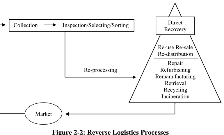
Figure 2-2, developed by de Brito and Dekker (2004), shows a network diagram of the processes involved in reverse logistics. It demonstrates how the four main activities can apply to any of the three main stages in the forward supply chain. After a product is
collected and goes through the inspection/selection/sortation process, it may enter the market through two different classifications. The first classification is made up of products that are undamaged or in a condition suitable for direct or second-hand sale. The second
Figure 2-2: Reverse Logistics Processes
In terms of the evolution of a reverse logistics system, companies tend to follow an ordered set of phases. Phase one is mainly in response to external forces such as government and customer requirements. During this phase, a company will start to deal with their own generated waste materials. In phase two, companies begin to branch out and develop formal recycling programs and work with legislators to establishing new guidelines and regulations. Phase three is when companies become competent in their reverse logistics systems and gain a competitive advantage. Phases two and three are mainly driven by top management
because they realize the value of environmental management (Martin, 2001).
2.3 Forward and Reverse Supply Chains
For many years, companies worked hard to build up and optimize their forward supply chains without giving much thought to what happened to products after their useful lives. Forward supply chains are composed of linear activities and logistics systems that are integrated to manufacture a raw material into a finished product and then distribute that
Re-use Re-sale Re-distribution
Repair Refurbishing Remanufacturing
Retrieval Recycling Incineration Collection Inspection/Selecting/Sorting Direct
Recovery
Market
product to an end-consumer. These unidirectional supply chains are called open loop supply chains (Realff, Ammons, & Newton, Robust Reverse Production System Design for Carpet Recycling, 2004). The typical open loop supply chain moves materials from supplier to manufacturer and then to wholesalers, retailers, and the final customer (Fleischmann & Minner, 2004). A forward supply chain is not concerned with what happens to the product after its disposal.
Analogously, reverse supply chains are composed of the reverse logistics systems and activities necessary for product recovery (Vachon, Klassen, & Johnson, 2001). Due to the three main driving forces of reverse logistics mentioned earlier, businesses have realized that reverse supply chains, utilizing reverse logistics principles and product recovery activities, are becoming increasingly important to stay competitive. Figure 2-3 shows the materials flowing through a reverse supply chain (Pochampally, Nukala, & Gupta, 2009).
Figure 2-3: Generic Reverse Supply Chain
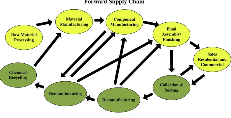
This is prompting companies to depart from the traditional, linear supply chain model into a cyclical, complex network model with feedback mechanisms (Fleischmann & Minner, 2004). These complex webs of interlinking forward and reverse supply chains are called closed loop supply chains (Realff, Ammons, & Newton, Robust Reverse Production System Design for Carpet Recycling, 2004). Figure 2-4, a modification of an established material flows diagram, shows the interconnectedness in a closed loop supply chain (Realff, Ammons,
Remanufactured Products Recycled
Goods Collection Consumers
Centers Recovery
Facilities Demand
Centers
& Newton, Strategic Design of Reverse Production Systems, 2000). Recycled products can reenter the forward chain through many different paths.
Figure 2-4: Generic Closed Loop Supply Chain
2.3.1 Feedback Mechanisms in Reverse Supply Chains
As supply chains are becoming more sophisticated, forward and reverse supply chains are becoming integrated into complex networks. Companies have discovered the value that can be gained by setting up systems designed to deliver inputs back into the manufacturing process or provide customers with a higher level of service. When companies choose to integrate reverse supply chains into their total supply chains, they must make a choice in their design. Reverse supply chains can be divided into two different categories based on
feedback mechanism. These are open loop or closed loop systems. Both are important for good product stewardship and material value recovery (Vachon, Klassen, & Johnson, 2001).
Component Manufacturing
Final Assembly/
Finishing
Sales Residential and
Commercial
Demanufacturing
Collection & Sorting Chemical
Recycling Raw Material
Processing
Material Manufacturing
Remanufacturing
Forward Supply Chain
Open loop and closed loop systems can be defined in two distinct ways, but both systems can ultimately be differentiated based on two different aspects of the product recovery phase. The first definition is concerned with who is active during the recovery phase, while the second definition focuses on where the recovered products end up after recycling. By the first definition, open loop systems are those set up by product
manufacturers that are not directly involved in the recovery process and remanufacturing of their products. These manufacturers may design their products for easy recycling, but a secondary market must exist to recover and convert these products into new ones. This is the type of system utilized by Apple Computers in the United States and Canada before 2001 (Apple, Inc., 2009). They did not take back their used computers directly, but encouraged other companies to make use of the used components (Vachon, Klassen, & Johnson, 2001).
Open loop systems are those that create products which will eventually be
can only be incinerated or landfilled. In this way, the value of the original materials become smaller and smaller until the value is completely lost.
In a closed loop system, using the first definition for the distinction between systems established earlier, the product manufacturer is directly involved in recovering its own goods for product or component life extension (Vachon, Klassen, & Johnson, 2001). This means that the same company is responsible for the distribution and recovery phases of their products’ life cycles (Blumberg, 2005). An example of this definition is the recovery of Mercedes-Benz engines. In 1997 Mercedes-Benz offered a program through their
dealerships where customers could choose to have a remanufactured engine installed in any vehicle model where the original engine could not be repaired or if the customer made a specific request. When the original engine was removed and replaced with a refurbished engine, the original engine was sent to a central refurbishment facility. After being
refurbished, the engine was warehoused until requested by a dealership (Driesch, van Oyen, & Flapper, 2005).
Newton, Carpet Recycling: Determining the Reverse Production System Design, 1999). One example would be the recycling of used PET bottles to make new PET bottles (Kiliaris, Papasphyrides, & Pfaendner, 2007).
The second use of closed loop systems is most often associated with
environmentalists and green thinkers. They have coined the phrase “cradle-to-cradle” to indicate the cyclical nature of a closed loop system. They see recycling as a method to reuse resources infinitely to limit resource depletion. Their view is that a closed loop system exists as long as recycled products are reused forever without being landfilled. However, the product does not necessarily have to be recycled and manufactured into the same product (Langenwalter, 2008). The result of the closed loop system is a loss of value because the product may be recycled into a lower form, but not a form that cannot be recycled later. An example of this takes place in the automotive recycling industry. A directive by the
2.3.2 Business Models
Even though different definitions exist for reverse logistics and closed loop supply chains, the central theme of product return leads to four main business models, which are defined below.
Basic reverse logistics model
Closed loop supply chain model for high tech products Closed loop supply chain model for low tech products Closed loop supply chain model that is consumer-oriented
The oldest and simplest of the four models, the basic reverse logistics model, is designed to return unwanted goods for processing and disposal. This model focuses on the economical disposal of wastes through landfilling or recycling. In the model, the manufacturers of the discarded products have no affiliation with the organization responsible for collection and disposal. Many companies profit from this business model including junk dealers, service organizations, and municipal waste collectors and recyclers (Blumberg, 2005).
The second business model, which is unique, integrates forward and reverse logistics to service high tech products because the original equipment manufacturer (OEM) has complete control of all forward and reverse activities. The OEM is responsible for servicing its products in the field. Any components that are replaced during service are refurbished and then placed back into the forward supply chain or sold into secondary markets
replaced, they could be refurbished and placed back into the supply chain (Blumberg, 2005). This business model is used to decrease the life cycle cost of very expensive products.
The third business model is similar to the second, but the OEM is not responsible for the entire closed loop supply chain; the forward and reverse supply chains are independent of each other. Generally the purchaser has more responsibility for the reverse supply chain. They may utilize third party logistics companies or their own resources for product recovery. In this business model, the purchaser is usually a large company with smaller dealers as distributors (Blumberg, 2005).
The fourth business model focuses on the consumer market. The responsibility of this closed loop supply chain is shared between the retailer and the OEM, and is unique in that two reverse logistic processes are designed to convey products from the OEM to the end user and back. Channels exist to return malfunctioning or unwanted products from the end user to the retailer, while another channel returns these same products from the retailer to the OEM. Likewise, products that expire or do not sell can be returned from the retailer to the OEM. This business model is utilized to link end users, retailers, and OEMs into a closed loop supply chain so that value can be recovered from failed, expired, or unwanted products (Blumberg, 2005).
2.3.3 What Makes Closed Loop Supply Chains Difficult
is present. The six major challenges that exist in the inventory control and production planning of a reverse supply chain are:
1. “Probabilistic recovery rate of parts from used products, which implies a high degree of uncertainty in material planning,
2. Unknown conditions of recovered parts until inspected, thus leading to stochastic routing and lead times,
3. Part-matching problem during the assembly process, 4. Added complexity of a remanufacturing shop structure, 5. Uncertainty in supply rate of used products, and
6. Problem of imperfect correlation between supply of used products and demand for reprocessed goods (Pochampally, Nukala, & Gupta, 2009).” Therefore, traditional production planning and scheduling methods for reverse supply chains have limited applicability. There is ongoing research to solve these problems, but either new methodologies must be created or classical methods revised (Pochampally, Nukala, & Gupta, 2009).
Another problem that arises is with the reverse portion of the closed loop supply chain. A company must decide to implement their own product recovery network or partner with companies that specialize in certain stages of the network. Putting together an entire collection and processing network can be very costly for a company, which encourages them to partner. However, problems arise with the successful collaboration of all players through the entire reverse network. Often information systems do not exist over the entire reverse supply chain and companies may be unwilling to share information with each other (Dyckhoff, Souren, & Keilen, 2004).
problem, manufacturers need to design their products with recovery in mind. They should focus on decreasing materials and material mixtures (Dyckhoff, Souren, & Keilen, 2004).
2.4 Recycling of Textile Materials
The previous section discussed four business models used in reverse supply chains. Currently, systems for the recovery of post-consumer textile materials utilize the first business model, which is the basic reverse logistics model. Collectors and recyclers do not have a direct link back to the manufacturer. Textile recycling supply chains have been developed primarily by entrepreneurs who have realized that they can profit from these reverse activities. Two reverse systems have emerged to recycle textile materials. Apparel recycling developed as a means to deal with castoffs created by continually-changing Western fashion (Hawley, 2006), while carpet recycling developed as a result of sustainability issues (Peoples, 2006).
2.4.1 Apparel Reverse Networks
The open loop reverse supply chain to recycle post-consumer apparel consists of consumers, policy makers, solid-waste managers, not-for-profit agencies, and for-profit retail businesses (Hawley, 2006). Apparel entering the reverse supply chain is primarily collected by charitable organizations such as Goodwill or the Salvation Army. In some instances, apparel may be sold to a second-hand shop or textile sorter. Whether the organization is charitable or for-profit, the apparel enters the first sortation phase. Charitable organizations and second-hand shops sort through the apparel to recover items to sell on their sales floors. Any apparel that does not sell or is discarded during the initial sortation is sold to textile sorting companies by the pound (Hawley, 2006). Prices often range from five to seven cents per pound (Rivoli, 2006).
Textile sorting companies, or “rag graders”, are primarily composed of small, family-owned businesses that are in their third or fourth generation of operation. When the
discarded apparel first enters these facilities, a rough sort is initiated which is aimed at separating heavy items and is performed by the least trained, newest employees (Hawley, 2006). Further sortation becomes more refined and is performed by graders with years of hands-on experience. These sorted items are then sold into specific markets. A large rag grading operation may have over four hundred distinct grades. For example, T-shirts alone can have over thirty separate categories (Rivoli, 2006).
regionally-dependent across the globe. Levi or Nike “diamonds” sold in Tokyo can bring textile sorters thousands of dollars in profit. Apparel that is deemed “vintage” can be sold by the piece and generates the largest profit. All other saleable apparel is consolidated into bales ranging in size from 500 to 1,000 pounds for export to foreign countries. For the nations of Sub-Sahara Africa, used clothing is a major American export. African customers can purchase T-shirts for twenty to twenty-five cents apiece (Rivoli, 2006).
Apparel that cannot be used as clothing enters several different channels. Depending on condition and fiber type, unwearable apparel may be transformed into wiping cloths, converted to value added products, or disposed of through landfilling or incineration
(Hawley, 2006). Cotton T-shirts are the primary source of wiping and polishing cloths. This is due to the soft and absorbent nature of cotton. The T-shirts, though not able to be worn, must contain fifteen square inches of material that is exclusive of tears, heavy stains, prints, or paint. Wiping cloths manufactures pay textile sorters about five cents per pound for this grade of apparel (Rivoli, 2006). For a small amount of the remaining apparel a niche market exists. These items can be converted into new apparel by designers and sold in trendy boutiques, which is popular in youth-oriented markets (Hawley, 2006).
manufactured into non-woven products. Examples of these products are garment linings, household and furniture items, insulation and sound absorbers, automobile carpeting, and toys. Expensive wool and cashmere fibers can be reclaimed and remanufactured into high-end blankets (Hawley, 2006). High quality cotton shoddy can be turned into lower-grade yarns for inexpensive clothing. Cotton shoddy can range in price from one to two cents per pound (Rivoli, 2006). Table 2-2, based on a table by Hawley (2006), shows the breakdown of the total volume of apparel after sortation, along with price.
Table 2-2: Volume to Value Estimation of Used Textile Product
Category
*Estimated Total Used Textile Goods by Volume
*Estimated Value Used Clothing Markets (Export) ~48% $0.50-$0.75 per pound. Conversion to Value Added
Markets
29% Value varies widely depending on product. Sold by weight. Wiping and Polishing Cloths 17% $0.80-$1.10 per pound Landfill and Incineration < 7% Varies by location and/or
rural/urban. Costs are by weight.
“Diamonds” 1-2% High value per item
Figure 2-5: Pyramid Model for Textile Recycling Categories by Quantity
Apparel recycling has been forced into a downcycling reverse supply chain for two main reasons, both a result of the advent of synthetic fibers. Due to increased fiber strength, it is difficult to re-open yarns without damaging fiber length. Also, it is difficult to separate re-opened fibers by type, especially when they are blends of natural and synthetic fibers (Hawley, 2006). Until new recycling technologies emerge, sorted apparel volume by
category will be inversely proportional to the value, as seen in Figure 2-5 which is based on a figure by Hawley (2006). Each tier of the pyramid represents the proportion of the total collected apparel volume by category.
2.4.2 Carpet Primer
Unlike apparel, carpeting is actually a complex system comprised of separate layers of functional elements. The majority of carpet (90%) is tufted, with two layers of backing. The face yarn, or pile, of the carpet is tufted into a woven, polypropylene (PP) primary backing. A thermosetting, calcium carbonate-filled (CaCO3) styrene-butadiene latex rubber
(SBR) is then applied to join a woven, polypropylene secondary backing to the primary
“Diamonds”
Landfill and Incineration
Wiping and polishing cloths
Conversion to new products
backing (Wang, Carpet Recycling Technologies, 2006). These two layers hold the tufted face yarns in place and add dimensional stability to the carpet system (Hilton, Construction and Fibers: Construction Basics, 2008).
Figure 2-6: Typical Carpet Construction
Figure 2-6 and Figure 2-7, from Wang, “Carpet Recycling Technologies” (2006), show the typical construction of a tufted carpet and the mass/area for the components in a typical tufted carpet, respectively. The total mass/area is 2,224 g/m2. Table 2-3, based on the information from Wang, “Carpet Recycling Technologies” (2006), shows the mass percentages for the components of a typical carpet.
Figure 2-7: Component Mass/Area for a Typical Carpet (g/m2)
Nylon is a strong polymer with good abrasion and crush properties, making it ideal for high traffic areas (Hilton, Construction and Fibers: Carpet Fibers, 2008).
Table 2-3: Component Mass Percentages for a Typical Carpet
Carpet Component Masses and Percentages Component Mass (g) % of Total Mass
Face Yarn 1018 45.77%
CaCO3 781 35.12%
Backing 221 9.94%
SBR 204 9.17%
Carpet sales are generally broken down into commercial and residential markets. Most carpet sold today in both markets is broadloom carpet construction which is typically sold by the square foot or meter, and comes in roll form. An important segment in the commercial market is carpet tile where construction is manufactured in flat squares that are typically nylon 6,6 (Realff, 2006). Table 2-4, by Realff (2006), shows the percentage of carpet sales in the United States by face fiber and markets.
Table 2-4: Approximate Distribution of Carpet Fiber by Face Type in the Commercial and Residential Sectors in the USA
Carpet Type by Face Fiber
% of Commercial Carpet
% of Residential Carpet Broadloom carpets
Nylon 6,6 60 35
Nylon 6 30 25
Polyester 10 15
PP 0 10
Other 0 5
Tile (30% of commercial sales)
2.4.3 Carpet Recycling History
In terms of post-consumer volumes and raw material recovery, carpeting represents a significant portion of the textile waste stream. The volume of carpet entering landfills has caused it to be the target of sustainability efforts. Early recycling efforts in the 1990s were the result of fiber producers realizing that real economic values were being lost as a result of landfilling carpet. In 1996, Dutch State Mines (DSM), Enichem, and the Organization of European Carpet Manufacturers, along with other partners, began a project known as the RECcling of CArpet Materials (RECAM). The project’s purpose was to design a European carpet waste recycling network (Louwers, Kip, Peters, Souren, & Flapper, 1999). In 1999, Honeywell and DSM opened a full-scale, post-consumer nylon 6 carpet processing plant in Augusta, Georgia (Peoples, 2006). The $85 million Evergreen Nylon Recycling facility was designed to recycle 200 million pounds of carpet into 100 million pounds of near-virgin caprolactam, the monomer that comprises nylon 6 (Canadian Textile Journal, 1999).
Polyamid 2000 filed for bankruptcy in June 2003. Both facilities were closed partly as a result of inefficient post-consumer carpet (PCC) collection networks in the United States and Europe (Peoples, 2006).
In 2001 an association of three states, Minnesota, Iowa, and Wisconsin, began discussions on diverting carpet from landfills. In 2002 a Memorandum of Understanding (MOU) was signed for the purpose of setting target dates and diversion rates of PCC from landfills. It also created a non-profit, third party organization, known as the Carpet America Recovery Effort (CARE), to oversee the ten year project. The MOU was a voluntary
agreement between signatory states, the United States Environmental Protection Agency, and non-governmental organizations to allow the project to be industry-led(Peoples, 2006).
CARE’s national goal is to increase the recycling and reuse amount of PCC to 40% by the year 2012. This means that 40% of all PCC disposed of annually will be diverted from the landfill (Carpet America Recovery Effort, 2006). CARE’s mission is to help facilitate the creation of a new industry in the United States without government regulations or subsidies. CARE is dedicated to building a group of interested individuals who can
low-value material shipments are avoided (Realff, Ammons, & Newton, Carpet Recycling: Determining the Reverse Production System Design, 1999).
2.4.4 Carpet Reverse Network
A post-consumer carpet (PCC) recycling network is comprised of the same elements as a basic reverse logistics model which contains:
Sites,
Recycling tasks, and
Transportation tasks (Realff, Ammons, & Newton, Carpet Recycling: Determining the Reverse Production System Design, 1999).
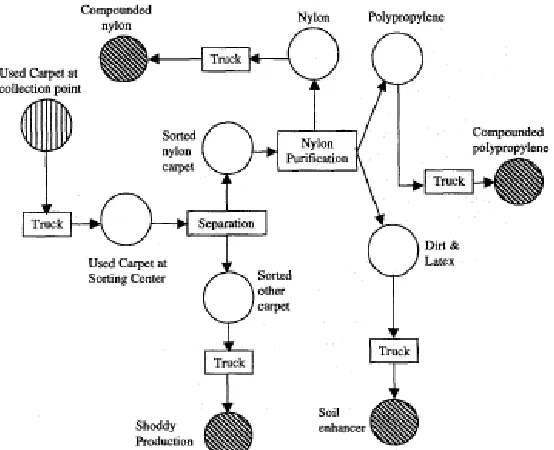
Sites represent the geographic locations where tasks are carried out. Knowing the locations of sites is important in the calculation of distances and methods of travel between sites. Recycling tasks are the reverse production processes that are performed at the sites. These include collection, sortation, separation, and mechanical/chemical recycling. The importance of this element is that all material enters unitarily and is broken down into fractions. All fractions of materials exiting a site in different streams must sum to one and match the incoming amount. Recycling tasks are assigned a cost which is dependent on the material flow per unit time.
Production System Design” (1999), shows the three basic elements formed into a network for recycling PCC.
Figure 2-8: Task Network for Carpet Recycling
2.4.4.1 Carpet Waste Forecasts and Collections
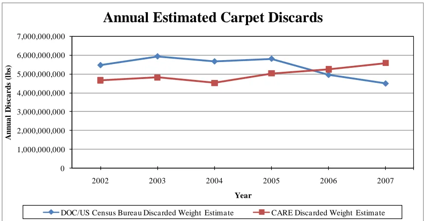
Basic estimations for annual PCC volumes are calculated from new carpet sales data and empirically-established national replacement rates, and is defined by the following formula:
Equation 2-1: Annual National Discarded Carpet Volume
In Equation 2-1, a simplified version of the equation defined by Realff (2006), V represents the national expected PCC volume, R represents the national replacement rate, and F
and the United States Census Bureau. These government agencies publish figures for annual shipments of carpets and rugs (United States Census Bureau, Manufacturing and
Construction Division, 2008). A more rigorous form of Equation 2-1 has been derived by Realff (2006) to account for regional differences in customer buying behavior and thus, discarded carpet volumes.
Equation 2-2: Annual Regional Discarded Carpet Volume