Locality Driven Memory Hierarchy Optimizations.

(1)

ABSTRACT

GUPTA, SAURABH. Locality Driven Memory Hierarchy Optimizations. (Under the direction of Huiyang Zhou.)

This dissertation first revisits the fundamental concept of the locality of references and proposes to quantify locality as a conditional probability: in an address stream, given the condition that an address is accessed, how likely the same address (temporal locality) or an address within its neighborhood (spatial locality) will be accessed in the near future. Based on this definition, spatial locality is a function of two parameters, the neighborhood size and the scope of near future, and temporal locality becomes a special case of spatial locality with the neighborhood size being zero byte. In previous research, some ad-hoc metrics have been proposed as a quantitative measure of spatial locality. In contrast, conditional probability-based locality measure has a clear mathematical meaning, offers justification for distance histograms, and provides a theoretically sound and unified way to quantify both temporal and spatial locality. The proposed locality measure clearly exhibits the inherent application characteristics, from which it is easy to derive information such as the sizes of the working data sets and how locality can be exploited. We showcase that our quantified locality visualized in 3D-meshes can be used to evaluate compiler optimizations, to analyze the locality at different levels of memory hierarchy, to optimize the cache architecture to effectively leverage the locality, and to examine the effect of data prefetching mechanisms.

(2)

donors for other co-scheduled workloads. We leverage our online locality monitoring to determine both the proper block size and the capacity assigned to each workload in a shared LLC. Our experiments show that our proposed approaches deliver significant energy savings in both single-core and multi-core processors.

Third, we propose a microarchitecture solution to enable cache bypassing for inclusive cache hierarchy designs. Recent works shows that cache bypassing is an effective technique to enhance the last level cache (LLC) performance. However, commonly used inclusive cache hierarchy cannot benefit from this technique because bypassing inherently breaks the inclusion property. We propose that bypassed cache lines can skip the LLC while their tags are stored in a ‘bypass buffer’. Our key insight is that the lifetime of a bypassed line, assuming a well-designed bypassing algorithm, should be short in upper level caches and is most likely dead when its tag is evicted from the bypass buffer. Therefore, a small bypass buffer is sufficient to maintain the inclusion property and to reap most performance benefits of bypassing. We show that a top performing cache bypassing algorithm, which is originally designed for non-inclusive caches, performs comparably for inclusive caches equipped with our bypass buffer. Furthermore, the bypass buffer facilitates bypassing algorithms by providing the usage information of bypassed lines to which reduces hardware implementation cost significantly compared to the original design.

(3)

(4)

Locality Driven Memory Hierarchy Optimizations

by Saurabh Gupta

A dissertation submitted to the Graduate Faculty of North Carolina State University

in partial fulfillment of the requirements for the degree of

Doctor of Philosophy

Computer Engineering

Raleigh, North Carolina 2014

APPROVED BY:

_______________________________ ________________________________ Eric Roternberg Xiaosong Ma

________________________________ ________________________________

Gregory Byrd Huiyang Zhou

(5)

ii

DEDICATION

(6)

iii

BIOGRAPHY

Saurabh Gupta was born to Shri Hari Om Gupta and Srimati Krishna Gupta in Kanpur, an industrial city in the state of Uttar Pradesh in India. He obtained his primary education in the city of Kanpur at schools including Pt. DeenDayal Upadhyay Sanatan Dharm Vidhyalaya. He has obtained his Bachelors and Masters in Electrical Engineering from Indian Institute of Technology Kanpur in 2009. Thereafter he joined Computer Engineering PhD program at NC State University in fall 2009.

(7)

iv

ACKNOWLEDGEMENTS

First and foremost I would like to acknowledge the support and encouragement of my parents and family to pursue my career goals and higher studies. Now, I would like to take this opportunity to acknowledge a lot of people who have contributed to my journey of finishing the formal education (loosely keeping them in a chronological order),

A job well begun is half done. I was lucky to start my education in the guidance of my father, my mother and my tutor, Anuj Sir. During high school, I admired the teaching style of Mahesh ji and Kailash ji who helped me attain good mathematical skills. During my year of break from school, Anish Sir and Pankaj Sir honed my command on physics and chemistry respectively to the competitive level. Also, I am grateful to my brothers/cousins, Sachin Gupta, Nirmit Gupta, Ramakant Gupta, Gaurav Gupta and Pradeep Gupta for being my best friends throughout my childhood. My friends from high school also had a great influence on shaping me and my career. I am especially thankful to Mayank Shukla, Suyash Mishra, Anunay Gupta, Srot Gupta, Ashish Kushwaha, Aditya Tiwari, Saurabh Awasthi, Abhinav Tripathi, Anurag Verma, Anurag Sharma, Pranjal Srivastava, Sugam Srivastava, Lokesh Dwivedi, Manoj Tripathi for being great friends. I am also thankful to Gaurav Gupta, Arun Koshta, Vikalp Sachan and Vikhyat Umrao for being there while we prepared for the toughest exam I ever wrote (at least it seemed so then). This led me to IIT Kanpur for my undergrad.

(8)

v

Tech. thesis student and Dr. S. S. K. Iyer in supporting my interdisciplinary thesis venture. I am also thankful to both of them for encouraging me to pursue a PhD program after my master degree. I would also like to thank Dr. S. P. Das and Dr. Rajat Moona for serving on my M. Tech. thesis committee at IIT Kanpur. Also, I am thankful to Dr. Y. N Singh and Dr. S. Qureshi for providing their recommendations with my application to PhD program.

Apart from academics at IIT Kanpur, my wing-mates including Purushottam Kar, Nikhil Saurabh, Vibhu Singh, Mayank Agarwal, Ravi Gupta, Vikas Sharma, Vishal Sharma, Suhail Rizvi, Prashant Saxena, Rajat Goyal, Soumya Banik, Pratibh Agarwal, Vivek Alok, Ankit Gupta, Samanvay Srivastava, Cherian Matthew, Shyam Sundar, Nipun Jain, Hemant Kumar, Vijay Bharti, Abhishek Sharma, Mayank Pandey, Vikas Saxena, Rohit Bishnoi, Vineet Dwivedi and Shreyansh Jain were the most motivating and supporting community I could have ever hoped for (B-mid ka tempo high hai). I would also like to acknowledge fellow EE student at IIT Kanpur including Ajit Pratap Singh, Mukund, Krishna Teja, K Ashwin, and Ashish Dembla. I had great time working with Deepak Ailani on my first ever research project and I was extremely blessed to have Nitin Munjal as my project partner for my first ever computer architecture course. I am especially thankful to Abhayendra Narayan Singh for helping me throughout my M. Tech. thesis with variety of things including application process for PhD program. At NC State, I survived my first semester with the guidance of Dr. Eric Rotenberg, Amit Qusba, Devesh Tiwari and Siddharth Chabbra. I also would like to thank Dr. Huiyang Zhou and Dr. Yan Solihin for very patiently talking to me at many occasions while I was trying to find a research focus to pursue for this dissertation.

(9)

vi

I would also like to thank Dr. Eric Rotenberg, Dr. Greg Byrd and Dr. Xiaosong Ma for serving of my dissertation committee and providing their critique as well as encouragement on my research projects. I have been a fan of the teaching style of Dr. Rotenberg and Dr. Byrd, and I want be appreciated as much by my students one day.

I had brilliant colleagues at NCSU. I would like to thank Nitin Kwatra, Pawandeep Singh Taluja, Sandeep Navada, Siddhartha Chabbra, Brandon Dwiel, Niket Chaudhary, Elliot Forbes, Ahmad Samih, Rami Al Sheikh, Amro Awad, Hiran Mayukh, Ganesh Balakrishnan, Yi Yang, Ping Xiang, Qi Jha, Xiangyang Guo, Yuan Liu, Hongwen Dai and Chao Li for being helpful during the course of my PhD program.

As they say, you are only as good as your company you keep. I am grateful to Devesh Tiwari, Rajeshwar Vanka, Amit Qusba, Avik Juneja, Raj Kumar, Rahul Ramasubramanian, Mahesh BV, Michelle Schisa, Aditya Deorha, Arpit Gupta, Santosh Navada, Sahil Sabharwal, Rohit Taneja and Ajit Narwal for being there at more personal level of friendship throughout these years. I must acknowledge Devesh’s ability to find related literature that always amazes me and has helped me on quite a few occasions. I would also like to thank Avik Juneja, Mahesh BV, Aditya Deorha, Santosh Navada, Ravi Komanduri, Kok Ren, Sriram PS and Neeraj Gole for being available for sports to keep my sanity. Special thanks to Arup Mazumdar, Dayanand Shaldhul and Mohit Gupta for tagging along with me on numerous road trips.

I am thankful to Linda Fontes, Elaine Hardin, Jennifer Raab and Kendall Del Rio for providing outstanding administrative support throughout the years. I cannot thank them enough for what they do for us as graduate students.

(10)

vii

LIST OF TABLES

(14)

xi

LIST OF FIGURES

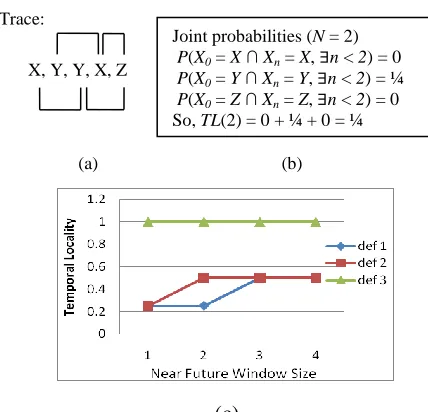
Figure 2.1. Calculating temporal locality. (a) Reference trace (also showing a moving future window of size 2); (b) Joint probability using Def. 1 of near future; (c) Temporal locality TL(N) using different

definitions of near future ... 8 Figure 2.2. The spatial locality plots of the benchmarks, mcf (SPEC2006) and

bzip2 (SPEC2000). Temporal locality is a special case of spatial

locality with neighborhood size as 0 ... 11 Figure 2.3. Spatial locality of the benchmark sphinx for neighborhood

definitions. (a) definition 1 (b) definition 2 ... 12 Figure 2.4. The Venn diagram showing the relationship among events X0 = A1,

X1 = A1 + ∆, and X2 = A1 ... 13

Figure 2.5. Locality and the difference functions for the benchmark hmmer. (a) Spatial Locality (b) Difference function over the near future window size N, which is the same as reuse distance histograms (c) Difference function over neighborhood size K, which shows a

histogram of stride access patterns ... 15 Figure 2.6. Locality for different matrix multiplication kernels (a) Untiled (b)

32x32 tile (c) 64x16 tile ... 19 Figure 2.7. The spatial locality of the benchmarks, art, mcf (SPEC 2000), and

bzip2 (SPEC2000) at different cache levels... 21 Figure 2.8. The spatial locality of L2 access traces for various benchmarks ... 23 Figure 2.9. The spatial locality for wupwise (a) L2 access trace (b) L2 miss

stream for 1MB L2 cache with a 64B block size (c) L2 miss stream for 1MB L2 cache with a 128B block size (d) L2 miss stream with a

stream buffer ... 25 Figure 2.10. Speedups of larger block sizes, next-n-line prefetching and

stream-buffer. ... 26 Figure 2.11. The spatial locality of L2 miss stream for the benchmarks (a)

equake; (b) lbm; (c) mcf (SPEC2000); and (d) milc ... 27 Figure 2.12. Performance improvements from the proposed buffers at the

memory controller level ... 28 Figure 2.13. The locality improvement of mcf and soplex at the L2 cache level (a)

(15)

xii

without the prefetcher, (d) the sub-trace locality of the L2 demand

trace of soplex with the prefetcher ... 30 Figure 2.14. The locality improvement at L2 cache from data prefetcher for milc,

hmmer, lbm and calculix shown by comparing the locality of demand access trace and sub-trace locality of demand accesses with

prefetcher ... 31 Figure 2.15. Locality of the LLC access stream for benchmarks (a) xalancbmk,

and (b) milc ... 35 Figure 2.16. IPC speedup of LRU, 3P-4P and DRRIP with different cache block

sizes over the baseline LLC with a 64-byte block size and the LRU

replacement policy ... 36 Figure 2.17. Different types of cache misses for LLCs with the block size of 64

bytes vs. 128 bytes ... 37 Figure 2.18. Weighted speedups of LRU, 3P-4P and DRRIP with different cache

block sizes (4MB LLC) over the baseline 4MB LLC with a 64-byte

block size and the LRU replacement policy ... 38 Figure 3.1: The locality plot of the benchmark gcc at L3 level ... 44 Figure 3.2: Organization of (a) ATDs and Locality Scores (LScores) for locality

computation (b) 2D-array of LScores per core ... 51 Figure 3.3: SLCP Architecture for LLCs ... 55 Figure 3.4. Normalized (a) L3 energy consumption, IPC Speedup and System

EDP for the Hcache algorithm and the Capacity_only scheme, and (b) L3 static/dynamic/total energy consumption, DRAM energy consumption, total energy consumption of the system for Hcache

algorithm ... 61 Figure 3.5. Normalized weighted speedup of UCP, UCP with static

128B/256B/512B cache block size and ALS ... 63 Figure 3.6. Normalized IPC throughput and weighted speedup of UCP, ALS,

PriSM and SLCP for 4-way multiprogrammed workloads... 64 Figure 3.7. Weighted speedup of UCP, ALS, PriSM and SLCP relative to the

baseline for 8-way multiprogrammed workloads and

geometric-mean summary for each category ... 66 Figure 3.8. (a) Normalized IPC throughput for UCP, ALS, UCP+ALS, and

SLCP over the baseline, (b) Normalized weighted speedup of UCP,

ALS, UCP+ALS and SLCP ... 67 Figure 3.9. Different hit rate curves used by UCP, PriSM and SLCP while

(16)

xiii

Figure 3.10. Variation of average WS improvement of SLCP with different

values of β parameter ... 70

Figure 3.11. Relative Power and Energy consumption of SLCP with respect to the baseline ... 71

Figure 3.12. Normalized IPC throughput of UCP, ALS, UCP+ALS and SLCP at L3 cache when ALS is applied at L2 cache ... 72

Figure 4.1. Memory hierarchy organization for (a) a non-inclusive LLC (b) an inclusive LLC (c) a non-inclusive LLC with bypass (selective fill of L3 cache) (d) an inclusive LLC with a bypass buffer to support cache bypassing ... 77

Figure 4.2. The lifetime histogram of the blocks, which are bypassed from the LLC, in the L1 data cache ... 80

Figure 4.3. Various fields present in a BB-entry ... 84

Figure 4.4. LLC miss rate comparison for different designs... 87

Figure 4.5. Fraction of bypassed LLC allocations for I-DSB-BBtracking ... 88

Figure 4.6. Fraction of bypassed blocks incurring a hit in the bypass buffer for I-DSB-BBtracking ... 88

Figure 4.7. Performance improvements of DSB, BB and I-DSB-BBtracking (w.r.t. the baseline inclusive LLC with the LRU replacement policy) ... 89

Figure 4.8. Performance of I-DSB-BB and I-DSB-BBtracking for different bypass buffer sizes ... 90

Figure 4.9. Performance improvements of DRRIP and I-DSB-BBtracking (w.r.t. the baseline inclusive LLC with the LRU replacement policy) ... 92

Figure 4.10. Performance improvements of DRRIP and I-DSB-BBtracking in presence of a stream buffer. The baseline is an inclusive LLC with the LRU replacement and a stream buffer prefetcher ... 93

Figure 4.11. Performance improvements of DSB, BB and I-DSB-BBtracking for different cache configurations. (the baselines are inclusive LLCs with the corresponding configurations) ... 94

Figure 4.12. Performance improvements of I-DSB-BBtracking and TA-DRRIP for a 4MB inclusive LLC for multi-programmed workloads (w.r.t. the baseline with the LRU replacement policy) ... 95

Figure 4.13. Comparing energy consumption of I-DSB-BBtracking with the baseline ... 96

(17)

xiv

Figure A.1. Locality plots for L3 access traces for SPEC2006 benchmarks ... 111 Figure A.2. Locality plots for L3 access traces for SPEC2006 benchmarks ... 112 Figure B.1. Sub-trace locality of L2 demand access traces for SPEC2006

benchmark ... 114 Figure B.2 Locality of L2 demand accesses and L2 miss traces in absence of

prefetching ... 115 Figure B.3. Locality of L2 demand accesses and L2 miss traces in absence of

(18)

1

Chapter 1

1. Introduction and Motivation

(19)

2

be exploited in various ways to improve performance or save energy consumption. This motivates the second chapter of this dissertation where we propose hardware mechanism to estimate spatial locality in an online fashion.

We present detailed architecture of online locality monitors to drive locality driven cache optimizations. Due to large area dedicated to last level caches, significant portion of static energy consumption is contributed by last level cache structure. Previous works focus on lowering cache consumption at little to no cost of performance degradation, such as [1]. Based on our spatial locality observation, we propose a novel cache reconfiguration algorithm to reduce cache energy consumption while improving cache performance. We also propose a novel approach to spatial locality aware cache partitioning for high performance. The cache partitioning has been proposed in the past to provide isolated capacity to each benchmark because uncontrolled management can lead to degraded performance of co-scheduled applications in a multicore system [52]. This problem has been approached from the temporal locality point-of-view in previous works by focusing on capacity management [12][52][56][61][65]. We make a case for using our proposed locality measure to analyze the spatial locality and temporal locality in runtime to drive spatial locality aware cache partitioning. In this manner, our proposed spatial-locality aware cache partitioning creates cache partitions which are heterogeneous in terms of cache block sizing as well as capacity. We show that this leads to significant improvement in performance and energy savings.

(20)

3

(21)

4

Chapter 2

2. Locality Principle Revisited: A

Probability-Based Quantitative Approach

2.1. Introduction

(22)

5

First, we propose to use conditional probabilities as a formal and unified way to quantify both temporal and spatial locality. For any address trace, we define spatial locality as the following conditional probability: for any address, given the condition that it is referenced, how likely an address within its neighborhood will be accessed in the near future. From this definition, we can see that the conditional probability depends on the definition of two parameters, the size of neighborhood and the scope of near future. Therefore, spatial locality is a function of these two parameters and can be visualized with a 3D mesh. Temporal locality is reduced to a special case of spatial locality when the neighborhood size is zero byte.

Second, we examine the relationship between our probability-based temporal locality and the reuse distance histogram, which is used in previous works for quantifying temporal locality. We derive that our proposed temporal locality (using one particular definition of near future) is the cumulative distribution function of the likelihood of reuse in the near future while the reuse histogram is the probability distribution function of the same likelihood, thereby offering theoretical justification for reuse distance histograms. The difference function of our proposed spatial locality over the parameter of the near future window size provides the reuse distance histograms for different neighborhood sizes. In comparison, the difference function of our proposed spatial locality over the parameter of the neighborhood size generates stride histograms for different near future window sizes.

Third, we use the proposed locality to analyze the effect of locality optimizations, sub-blocking/tiling in particular. The quantitative locality presented in 3D meshes visualizes the locality changes for different near future windows and neighborhood sizes, which helps us to evaluate the effectiveness of code optimizations for a wide range of cache configurations.

(23)

6

replacement policy. Given the importance of last-level caches (LLCs) in multi-core architectures, we also present a detailed locality analysis to make a case for LLCs with large block sizes and relatively simple replacement policies.

Our proposed locality measure clearly presents the characteristics of a reference stream and helps to reveal interesting insights about the reference patterns. Besides locality analysis, another commonly used way to understand the memory hierarchy performance of an application is through cache simulation. Compared to cache simulation, our proposed measure provides a more complete picture since it provides locality information at various neighborhood sizes and different near future window scopes while one cache simulation only provides one such data point.

The remainder of this chapter is organized as follows. Section 2.2 defines our probability-based locality, derives the difference functions, and highlights the relationship to reuse distance histograms. Section 2.3 focuses on quantitative locality analysis of compiler optimizations for locality enhancement. Section 2.4 discusses locality analysis of cache hierarchies and presents how the visualized locality reveals interesting insights about locality at different levels of cache hierarchy and about data prefetching mechanisms. We also highlight how the locality information helps to drive memory hierarchy optimizations. Section 2.5 presents a GPU-based parallel algorithm for our locality computation. Section 2.6 discusses the related work. Finally, Section 2.7 summarizes the key contributions of this chapter.

2.2. Quantifying Locality of Reference Using Conditional Probabilities

2.2.1. Temporal Locality

Temporal locality captures the characteristics of the same references being reused over time. We propose to quantify it using the following conditional probability: given the condition that an arbitrary address, A, is referenced, the likelihood of the same address to be re-accessed in the near future. Such conditional probability can be expressed as P(Xn = A, n

(24)

7

future. Since an address stream usually contains more than one unique address, the temporal locality of an address stream can be expressed as a combined probability, as shown in Equation 1, where M is the number of unique addresses in the stream.

( | )

∑ ( | ) ( ) Eq. 1

Equation 1 can be further derived using Bayes' theorem, shown as Equation 2.

∑ ( ) Eq. 2

To calculate the joint probabilities, P(Xn = Ai, n in near future ∩ X0 = Ai), we need to

formulate a way to define the term ‘near future’. We consider three such definitions and represent temporal locality as TL(N) = P(Xn = A, n < N| X0 = A), where N is the scope of

the near future or the future window size.

Def. 1 of near future: the next N addresses in the address stream.

Def. 2 of near future: the next N unique addresses in the address stream.

Def. 3 of near future: the next N unique block addresses in the address stream given a specific cache block size. In other words, we ignore the block offset when we count the next N unique addresses.

Based on the definition of the near future, the joint probability P(X0 = A ∩ Xn = A, n <

N) can be computed from an address trace with a moving near future window. In a trace of the length S, for each address (i.e., the event X0 = A), if the same address is also present in

the near future window (i.e., the event Xn = A, n < N), we can increment the counter for the

joint event (X0 = A ∩ Xn = A, n < N). After scanning the trace, the ratio of this counter over

(S – 1) is the probability of P(X0 = A ∩ Xn = A, n < N). The reason for (S – 1) is to account

(25)

8

trace. During the scan through the trace, if def. 1 of near future is used, the moving window has a fixed size while def. 2 and def. 3 require a window of variable sizes. We illustrate the process of calculating temporal locality with an example shown in Figure 2.1.

(c)

Figure 2.1. Calculating temporal locality. (a) Reference trace (also showing a moving future window of size 2); (b) Joint probability using Def. 1 of near future; (c) Temporal locality TL(N) using different definitions of near future.

Considering the trace shown in Figure 2.1, for each address (except the last one), we will examine whether there is a reuse in its near future window. If the near future window size is 2 and we use Def. 1 of near future, we will use a window of size 2 to scan through the trace as shown in Figure 2.1a. Based on the joint probabilities, the temporal locality, TL(2), is ¼ as shown in Figure 2.1b. If we follow Def. 2 of near future, the temporal locality, TL(2), is 2/4 since each near future window will contain 2 unique addresses. If we use Def. 3 of near future and assume that X, Y, and Z are in the same block, the temporal locality, TL(2), is 1. The temporal locality with various near future window sizes is shown in Figure 2.1c for these three definitions of near future.

Joint probabilities (N = 2)

P(X0 = X ∩ Xn = X, n < 2) = 0

P(X0 = Y ∩ Xn = Y, n < 2) = ¼

P(X0 = Z ∩ Xn = Z, n < 2) = 0

So, TL(2) = 0 + ¼ + 0 = ¼ Trace:

(b)

(26)

9

2.2.2. Spatial Locality

Spatial locality captures the characteristics of the addresses within a neighborhood being referenced over time. We propose to quantify it as the following probability: given the condition that an arbitrary address, A, is referenced, the likelihood of an address in its neighborhood to be accessed in the near future. Such conditional probability can be expressed as P(Xn in A’s neighborhood, n < N | X0 = A), where X0 is the current reference

and Xn is a reference in the near future. Similar to temporal locality, the spatial locality of an

address stream can be computed as the combined probability of all the unique addresses in the trace and it can be expressed as Equation 3, where M is the number of unique addresses in the stream.

( | )

∑ ( | ) ( )

∑ ( ) Eq. 3

To compute the joint probabilities, ( ) we need to define the meaning of the term ‘neighborhood’ in addition to near future. We consider two definitions for neighborhood and represent spatial locality as SL(N, K), where N is the near future window size and K is a parameter defining the neighborhood size.

Def. 1 of neighborhood: an address X is within the neighborhood of Y if |X – Y| < K, where 2*(K – 1) is the size of the neighborhood. The reason for 2*(K – 1) rather than (K – 1) is to account for the absolute function of (X – Y).

Def. 2 of neighborhood: two addresses X and Y are in the same cache block given the cache block size as K. In other words, X is within the neighborhood of Y if X – (X mod K) = Y – (Y mod K).

(27)

10

addresses while for spatial locality, the addresses in the window are inspected to see whether there exists a reference Xn , n < N, falling in the neighborhood of X0. If we change the

definition of neighborhood size to zero (i.e., K = 1), spatial locality is reduced to temporal locality.

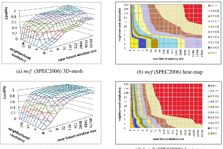
From Equation 3, we can see that spatial locality is a function of two parameters, the neighborhood size, K, and the near future window size, N. As such, we can visualize the spatial locality of an address stream with a 3D mesh or a 2D heat-map for different neighborhood and near future window sizes. Figure 2.2 shows the spatial locality, using the def. 2 of near future and def. 1 of neighborhood, of the benchmarks SPEC2006 mcf and SPEC2000 bzip2 (see the experimental methodology in Section 2.4.1). Temporal locality is the curve where the neighborhood size is zero.

Locality visualized in 3D meshes or heat-maps clearly shows the characteristics of reference streams. First, a contour in the 3D mesh/heat-map at a certain locality score (e.g., 0.9) can be used to figure out the sizes of an application’s working data sets. Comparing Figures 2.2b to 2.2d, it is evident that bzip2 has a much smaller working data set than mcf. We can also see that the size of the working set varies for different neighborhood sizes. For example, SL(8192, 32) of mcf is close to 0.9, indicating the working set size is slightly bigger than 2*32B*8192 = 512kB when the neighborhood size is 64 (= 2*32) bytes. On the other hand, SL(65536, 16) of mcf is little less than 0.9, showing that the working set is greater than (2*16B*65536) = 2 MB when the neighborhood size is 32(=2*16) bytes.

(28)

11

accumulative. In other words, a reuse within a small neighborhood (or close future) is also a reuse for a larger neighborhood (or not-so-close future).

Third, our proposed locality can be used to reveal interesting insights which are typically not present through cache simulations because one cache simulation only provides one data point in this 3D mesh. As one example, the benchmark, hmmer, shows steps in the locality scores (Figure 2.5a) when the near future size is at 32 and 8192, which implies that there is a good amount of data locality that we cannot leverage until we can explore the reuse distance of 8192. Such observations from the 3D mesh enable us to understand why and whether a particular cache configuration performs much better than the other ones.

Between heat maps and 3D meshes, locality presented in heat-maps better reveals the working set information. On the other hand, 3D-meshes are more useful in showing how the

(c) bzip2 (SPEC2000) 3D-mesh (a) mcf (SPEC2006) 3D-mesh

(d) bzip2 (SPEC2000) heat-map

Figure 2.2. The spatial locality plots of the benchmarks, mcf (SPEC2006) and

bzip2 (SPEC2000). Temporal locality is a special case of spatial locality with nighborhood size as 0.

(29)

12

locality changes along either the neighborhood size or the near future window size, which indicates how the locality can be exploited.

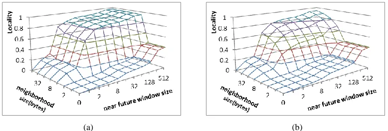
Different definitions of ‘near future’ lead to different near future window sizes as illustrated in Figure 2.1. Such differences, however, turn out to have little impact when we compute locality for most SPEC CPU benchmarks. Between the two definitions of neighborhood, although def. 2 models the cache behavior more accurately, it fails to capture spatial locality across the block boundary. For example, for a perfect stride pattern, 1, 2, 3, 4, 5, …, the spatial locality using neighborhood def. 1 will be 1 for any neighborhood size and any future window size greater than 0. If we use def. 2 of neighborhood, the spatial locality will be dependent upon the neighborhood (or cache block) size. If the neighborhood/block size is 2 bytes, the spatial locality is 0.5 for any future window size. If the neighborhood/block size is B bytes, the spatial locality becomes (B – 1)/B for any future window size greater than or equal to B. In Figure 2.3, we show the spatial locality for the benchmark sphinx with neighborhood def. 1 (Figure 2.3a) and def. 2 (Figure 2.3b). From the figure, we can observe the similar behavior, i.e., increasing locality values for larger neighborhood sizes in Figure 2.3b. In contrast, Figure 2.3a shows a stepwise increase in locality values. Based on these observations, we choose to use def. 2 of near future and def. 1 of neighborhood for locality analysis. Whenever the objective is to estimate the cache performance, def. 3 of near future and def. 2 of neighborhood can be used instead.

(a) (b)

(30)

13

2.2.3. The Relationship between Spatial and Temporal Locality

Based on our probability-based definitions of spatial and temporal locality, temporal locality can be viewed as a special case of spatial locality. Beyond this observation, there also exist some intriguing subtleties between the two types of locality. In particular, we can change the neighborhood definition in spatial locality so that the exact same addresses are excluded from the neighborhood. In other words, the neighborhood definition becomes 0 < |X – Y| < K. In this case, an interesting question is: for any address trace, is the sum of its spatial locality and its temporal locality always less than or equal to 1?

An apparent answer is yes since the reuses from the same addresses are excluded from the neighborhood definition. This is also our initial understanding until our locality computation results show otherwise. After a detailed analysis, it is found that the events for temporal and spatial locality are not always disjoint and therefore the sum can be larger than 1. To elaborate, we use def. 1 of near future and def. 1 of neighborhood with the modification that same addresses being excluded. Other definitions of the two terms can be applied similarly. Following Equations 1 and 3, temporal and spatial locality can be expressed as the following two conditional probabilities: P(Xn = A, | X0 = A) and P(0 < |Xn – A| <

K, | X0 = A), respectively. Both probabilities can be computed using the sum of the

joint probabilities ∑ (Xn = Ai, ∩ X0 = Ai) and ∑ (0 < |Xn – Ai| < K,

X0 = A1

X2 = A1

X1 = A1+∆

(31)

14

∩ X0 = Ai). Since each Ai is unique, the events X0 = Ai are disjoint for different Ai.

So, we can focus on one such address, e.g., A1. We can use the Venn diagram to capture the

relationship among the events: X0 = A1, X1 = A1 + ∆, and X2 = A1, as shown in Figure 2.4.

From Figure 2.4, we can see that (X0 = A1∩ X2 = A1) and (X0 = A1∩ X 1 = A1 + ∆) are not

disjoint. An intuitive explanation is that for an address sequence such as A1, A1+1, A1, the

third reference (A1) contributes to both temporal locality of the first reference and spatial

locality of the second reference. Therefore, the events for temporal and spatial locality are not disjoint although the references to same addresses are excluded from the neighborhood definition.

2.2.4. Difference Functions of Locality Measures and the Relationship to Reuse

Distance Histograms

Next, we derive the relationship of our probability-based temporal locality to reuse distance histograms, which are commonly used in previous works to quantify temporal locality. In sequential execution, reuse distance is the number of distinct data elements accessed between two consecutive references to the same element. The criterion to determine the ‘same’ element is based on the cache-block granularity, i.e., the block offsets are omitted when determining reuses. The reuse distance provides a capacity requirement for fully associative LRU caches to fully exploit the reuses. The histogram of reuse distances is used as the quantitative locality signature of a trace since it captures all the reuses at different distances.

Based on our probability-based measure, temporal locality TL(N) represents the probability P(Xn = A, n < N| X0 = A). As this probability is a discrete function of N, we can

take a difference function of temporal locality ∆TL(N) = TL(N) – TL(N – 1) = P(XN-1 = A | X0

= A). This function represents the frequency of reuses at the exact reuse distance of (N – 1). If we use def. 3 of the term near future, the difference function becomes: ∆TL(N) = P(XN-1 =

block_addr(A) | X0 = A) where block_addr(A) = A – (A mod block_size) and it is essentially

(32)

15

the probability distribution function of the event (XN-1 = A | X0 = A) and our proposed

temporal locality is the accumulative distribution function of the same event.

As spatial locality, SL(N, K), is a function of two parameters, the near future window size N and the neighborhood size K, we can compute the difference function of SL(N, K) over either parameter and both difference functions reveal interesting insights of the access patterns. Similar to temporal locality, the difference function of spatial locality over N, SL(N, K) – SL(N – 1, K) = P( (XN-1 – XN-1 mod K) = (A – A mod K) | X0 = A), shows the reuse

distance histograms with different block sizes, K, if we follow def. 2 of neighborhood.

(b) (c)

Figure 2.5. Locality and the difference functions for the benchmark hmmer. (a) Spatial Locality (b) Difference function over the near future window size N, which is the same as reuse distance histograms (c) Difference function over neighborhood size K, which shows a histogram of stride access patterns.

(33)

16

The difference function over the neighborhood size parameter, K, can be derived as follows: SL(N, K) – SL(N, K – 1) = P(|Xn – A| = K – 1, n < N | X0 = A). This probability

function represents that in an address trace how often a stride pattern with a stride of (K – 1) happens in a near future window of size N. For different N and K, this function essentially provides a histogram of different strides for any given near future window size. In the context of processor caches, this difference function helps to reason about the relationship among the cache sizes, which determine the maximum reuse distance or near future window size, the block sizes, which determine the neighborhood sizes, and the performance potential of stride prefetchers.

In Figure 2.5, we present the spatial locality information (Figure 2.5a) of the benchmark, hmmer, and its two difference functions (Figures 2.5b and 2.5c). From the Figure 2.5b, we can see how the reuse distance histograms vary for different block sizes. For small block sizes, many reuses can only be captured with long reuse distances. For large block sizes, the reuse distance becomes much smaller. This clearly indicates that one reuse histogram is not sufficient to understand the reuse patterns. Based on Figure 2.5c, we can see that for small near future windows, there are limited stride accesses. When the near future window size increases (larger than 32), the stride access pattern (stride of 8 bytes) is discovered. It implies that although the application has strong spatial locality in the forms of stride access patterns, in order to exploit such spatial locality, the cache size and set associativity need to be large enough to prevent a cache block from being replaced before it is re-accessed. In addition, the single dominant stride suggests that a stride prefetcher can be an effective way to improve the performance for this benchmark.

2.2.5. Sub-trace Locality

(34)

17

locality is usually not the same as the locality computed from the filtered trace, e.g., the addresses generated by one instruction, because the filtered trace will miss the constructive cross-references from other instructions. Instead, sub-trace locality is computed from the ‘whole’ trace. Mathematically, sub-trace spatial locality (STSL) can be defined and derived as the sum of the joint probabilities as shown in Equation 4. Sub-trace temporal locality (STTL) can be derived similarly.

( | )

∑ (

) Eq. 4

From Equation 4, it can be seen that compared to whole trace locality, sub-trace locality is modeled with the additional joint events, ( ), in the joint probability computation. The definition of SetX and SetY determines the event of interest. For example, to compute the locality of one particular memory access instruction, we can define SetX as {the addresses generated by the instruction of interest} and define SetY as the whole sample space Ω or {addresses generated by all instructions}, meaning that for all the addresses (i.e., ( )), we need to check whether there is a spatial reuse in the near future by the instruction of interest ( h h h ) If we change SetY to SetX, the equation calculates the locality of the address trace generated by the instruction of interest (i.e., the filtered trace).

We can make a slight change to Equation 4 so that it can be computed more efficiently. Instead of looking for reuses in a near future window, we can use a near past window, as shown in Equation 5. This way, we can compute the locality of an instruction of interest as follows, for each address generated by the instruction (i.e., the event: ), we search in a near past window for spatial reuse (i.e., the event:

.)

∑ (

(35)

18

Another use of sub-trace locality is to analyze the effectiveness of data prefetching. For example, consider the following address trace containing both demand requests (underlined addresses) and prefetch requests: A, A+32, A+64, A+96, A+128, A+64, A+128, A+160, A+192. In this case, we can define SetX = {demand requests} and SetY = {combined demand and prefetch requests}. Then, sub-trace locality provides the information that for a demand request, how likely there are prefetch requests (or demand requests) for the same address in a near past window. The locality of either the demand request trace or the combined demand and prefetch request trace does not provide such information.

2.3. Locality Analysis for Code Optimizations

In this section, we use sub-blocking / tiling to show how our proposed measure can be used to analyze and visualize the locality improvement of code optimizations.

To analyze the locality improvement of the sub-blocking/tiling optimization, we choose to use the matrix multiplication kernel C = A x B and we use the pin tool [46] to instrument the binaries to generate the memory access traces for our locality computation. We used def. 1 of near future and def. 1 of neighborhood in our locality computation. Figure 2.6 shows the locality information collected for different versions of the kernel, including un-tiled, tiled with the tile size of 32x32, and the tiled with the size 64x16. The matrix size is 256x256.

(36)

19

= 128k accesses, which is why temporal locality for the maximum near future value in Figure 2.6a is still around 50%. Since the matrix B is accessed column-wise, with the near future window size of 1024 and neighborhood size of 4, accesses to the matrix B start to enjoy spatial locality (i.e., B[i][j] and B[i][j+1] show in the same window) and the locality becomes very close to 1 as shown in Figure 2.6a.

With the loop tiling optimization, both matrices A and B are divided into tiles/sub-blocks. This reduces the reuse distance of the data elements as we can see from Figures 2.6b and 2.6c. For a tile size of 32x32, the inner loops perform matrix multiplication of two 32x32 matrices. As a result, the sub-blocks of A get reused when the near future window is larger than 64 and the sub-blocks of B get reused when the near future window is 2048 (= 32x32x2). The sub-blocks of matrix A are accessed row-wise and show 0.5 spatial locality when the neighborhood size is 4 bytes and near future window is smaller than 64. The sub-blocks of the matrix B show spatial locality when the near future window is larger than 64, which makes B[ii][jj] and B[ii][jj+1] show up in the same window. The 3D locality mesh shown in Figure 2.6b visualizes these changes in both temporal and spatial locality and confirms the observations. When the tile size is 64x16, the locality information, shown in Figure 2.6c, is the same as matrix multiplication of a 64x16 matrix with a 16x64 matrix.

Based on the locality information shown in Figure 2.6, we can easily see how much and where the locality improvement has been achieved with code optimizations. Furthermore, if

(a) (b) (c)

(37)

20

we use def. 3 of near future and def. 2 of neighborhood, we can also use our locality function to infer how much locality a specific cache can capture. For example, an 8kB cache with a 16-byte block size will be able to explore the future window up to 512 (8kB/16 bytes) and neighborhood range of 16 bytes. Therefore, SL(512, 16) will show the hit rate of this cache if it is fully associative. Mathematical models proposed in [8][31][58] can also be used to estimate miss rates for set-associative caches from the fully associative ones.

2.4. Locality Analysis for Memory Hierarchy Optimizations

Our proposed locality measure provides quantitative locality information at different neighborhood sizes and near future scopes. In this section, we show that it reveals interesting insights to drive memory hierarchy optimizations.

2.4.1. Experimental Methodology

In this section, we use an in-house execution driven simulator developed based on SimpleScalar [7] for our study, except stated otherwise in Section 2.4.4 and Section 2.4.6. In our simulator, we model a 4-way issue superscalar processor. The memory hierarchy contains a 32kB 4-way set-associative L1 data cache with the block size of 64 bytes (3 cycle hit latency), a 32kB 2-way set associative L1 instruction cache, and a unified 8-way set associative 1MB L2 cache with the block size of 64 bytes (30 cycle hit latency). The main memory latency is set as 200 cycles (224 cycles) to get a 64-byte (128-byte) L2 block. The memory bus runs at 800MHz while the processor core runs at 2GHz.

(38)

21

2.4.2. Locality at Different Memory Hierarchy Levels

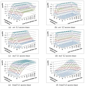
In this experiment, we examine the locality of the L1 data cache access trace and the L2 cache access trace. We use the benchmarks art, mcf (SPEC2000) and bzip2 (SPEC 2000) as our case studies. Figure 2.7 shows the locality of L1 and L2 access traces for art, bzip2, and mcf.

By comparing Figures 2.7a to 2.7b, 2.7c to 2.7d and 2.7e to 2.7f, we can see that the L1 cache effectively exploits the spatial locality with neighborhood size less than 64 bytes (K =

(a) art L1 access trace (b) art L2 access trace

Figure 2.7. The spatial locality of the benchmarks, art, mcf (SPEC 2000), and

bzip2 (SPEC2000) at different cache levels.

(39)

22

32), which is the L1 block size. Also, the capacity of the L1 cache enables it to exploit a near future window of 512 (=L1 size/block size). As a result, at the L2 level, there is limited locality present in this range. So, in order for L2 to become effective, it has to support much larger near future windows (by a large L2 cache size) and/or larger neighborhood sizes (by a large L2 block size). For the benchmark art, we can see from Figure 2.7a that the locality does not increase much as we increase the near future window size up to 32768. If we keep the L2 cache block size the same as the L1 block size, the gains by increasing the cache size is very limited until it can explore the near future window size of 32768 (implying a L2 cache size of 32768 x 64B= 2MB) as shown in Figure 2.7a. While making the cache block size 128B will significantly improve the spatial locality exploited by L2 cache. For the benchmark mcf, similar observations can be made from the locality curve. For the benchmark bzip2, the spatial locality of the L2 accesses is lower than the other two benchmarks in Figure 2.7.

At lower levels of caches in a cache hierarchy, the accesses seen are primarily the misses from upper levels. This causes the lower levels to have no spatial locality until they have block sizes bigger than upper levels.

2.4.3. Memory Hierarchy Optimizations

1) Optimizing Last-Level Caches (LLCs):

(40)

23

However, in many current commercial processors, the same cache block size (e.g., 64 bytes in Intel Core i7) is used for different level of caches to simplify the cache coherence

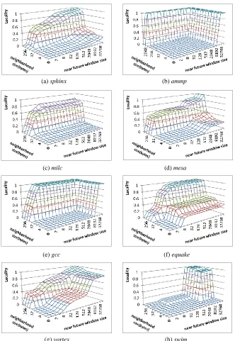
Figure 2.8. The spatial locality of L2 access traces for various benchmarks.

(g) vortex (h) swim

(e) gcc (f) equake

(c) milc (d) mesa

(41)

24

management. From the locality information shown in Figure 2.8 and Figure 2.9a, we can see that many benchmarks require much larger neighborhood sizes to take advantage the spatial locality. Among these benchmarks, wupwise, milc, mesa, equake, vortex and gcc would need the neighborhood size of 64 bytes (i.e., 128-byte cache block) while sphinx, mcf and art exhibit additional spatial locality for increasing neighborhood sizes. The benchmark, ammp, requires a neighborhood size of 2048 bytes due to its streaming access pattern with a stride of more than 1024 bytes.

Second, for all these benchmarks, the spatial locality can be exploited within a small near future window (or reuse distance) when a large block is used. This indicates that a small cache with relatively large block sizes can be more effective than a large cache with small block sizes. For example, for benchmark gcc, SL(4,64) = 0.97 (corresponding to a 4x128 = 512 byte cache with the 128-byte block size) is higher than SL(8192,32) = 0.008 (corresponding to a 8192 * 64 = 512KB cache with a 64-byte block size) and is very close to SL(16384, 32) = 0.99 (corresponding to a 16384*64 = 1MB cache with a 64-byte block size). Since most of the locality can be captured within a small near future window, it also means that the LRU replacement policy will work well for caches with large blocks, thereby eliminating the need for more advanced replacement policies (more discussion in Section 2.4.6). Furthermore, the limited near future window indicates that the required set associativity is small as well.

(42)

25

2kB/64B = 32. In other words, our locality measure can be used a profiling tool to control the next/previous-n-line prefetching. The advantage of this approach is that it can emulate different cache block sizes without changing the cache configurations (i.e., cache size, set associativity, and block size). The third way is to use a stream buffer to detect stride patterns and prefetch data blocks into caches.

Next, we evaluate and compare the effectiveness of these different approaches using our locality measure with a case study of the benchmark wupwise. Here we use the locality measure of the L2 demand miss stream as it shows the locality that the L2 cache fails to exploit. In Figures 9b, 9c, and 9d, we show the L2 miss locality measure for wupwise when the L2 cache uses a 64-byte block size, a 128-byte block size, and a stream-buffer. The next/previous line prefetch has very similar results to the cache with the 128-byte block size.

Figure 2.9. The spatial locality for wupwise (a) L2 access trace (b) L2 miss stream for 1MB L2 cache with a 64B block size (c) L2 miss stream for 1MB L2 cache with a 128B block size (d) L2 miss stream with a stream buffer.

(c) (d) (c)

(43)

26

From Figure 2.9b, we can see that the L2 cache with a 64-byte block size fails to exploit the spatial locality at large neighborhood sizes. In contrast, Figure 2.9c shows that the 128-byte block cache with the same size exploits the spatial locality effectively. The stream prefetcher does not work as well for wupwise as the stride access patterns are not common in this benchmark (Figure 2.9d). Our timing simulation also confirms the similar trend in performance improvement for wupwise: an execution-time reduction of 5% using the stream buffer while the 128-byte block size and next line prefetching achieve the execution-time reduction of 11% to 14%, respectively.

Figure 2.10 shows performance improvements measured in IPC (instructions per cycle) speedups for large block sizes, next/previous-n-line prefetching, and stream buffer prefetcher. Among the benchmarks, equake, gap, hmmer, mcf(SPEC2000), mcf (SPEC2006), milc, parser, perl, and wupwise favor large block sizes (or previous/next-n-line prefetching). On average, 4.7% (6.6%) IPC improvement is achieved on average across all the benchmarks using large block sizes (previous/next-n-line prefetching). Benchmark swim experiences a slowdown when bigger block size or next/previous-n-line prefetching is used. The results can be explained with the locality of its L2 access trace (Figure 2.8i). From the figure, we can see that the difference in locality score, when the block size is changed from 64 bytes to 128 bytes, is very small for swim. Therefore, the increased latency to get a larger

(44)

27

data block results in a slowdown. Benchmarks ammp, art, gap and lbm have stride beyond 64 bytes, therefore 128 byte block size is not much helpful for these benchmarks. We determine the more suitable ‘n’ value to be used in next/previous nth-line prefetcher from the locality measure. For most benchmarks, the next/previous nth-line prefetching successfully emulates the bigger cache block size. On the other hand, the benchmarks ammp, bzip2(SPEC2000), bzip2(SPEC2006), gcc, gromacs, lbm, sphinx, swim and vortex benefit more from the streaming buffer and it shows 17% performance gains on average across all the benchmarks.

2) Optimizing Memory Controller:

Even with the spatial locality being leveraged by large blocks or stream buffers, when we examine the locality of the L2 demand miss stream, we observe that there is residual locality to be leveraged. As an example, Figure 2.11a shows the locality information for the demand memory access stream of the benchmark equake when the L2 cache has the cache line size of 128 bytes. From the locality measure, it can be seen that there exists strong spatial locality

Figure 2.11. The spatial locality of L2 miss stream for the benchmarks (a) equake; (b) lbm; (c) mcf (SPEC2000); and (d) milc.

(a) equake (b) lbm

(45)

28

when the neighborhood size is larger than 256 bytes (K = 128). Although DRAM system can exploit some of this locality in the DRAM row-buffer, where a row-buffer hit has significantly lower latency than a row-buffer miss, our locality measure reveals further insights on how to better exploit the locality. From Figure 2.11a, we can observe that with a short near future window of 1 reference, the locality score SL(1, 256) is 0.29 for equake. When increasing the near future window size to 4 references, the locality score SL(4, 256) for equake is increased to 0.54. Similarly, the benchmarks, lbm, mcf (SPEC2000) and milc, have significantly higher locality for near future window sizes larger than 1 (Figure 2.11b, 2.11c and 2.11d). Based on this observation, we propose to add a small buffer at the memory controller level. This buffer has large block sizes (e.g., 1kB to 4kB) but with just a few entries (e.g., 4).

Compared to the row buffer in the DRAM, which can be viewed as an off-chip single-entry buffer with a block size of 4kB, it has two benefits: (1) a multi-single-entry buffer is able to exploit the significantly higher locality present beyond the near future scope of 1 reference, and (2) a buffer located at the on-chip memory controller has much lower latency than the off-chip DRAM row buffer. For the benchmarks showing no such spatial locality, we can simply power-gate this small buffer.

(46)

29

In our experiment, we use a 4-entry buffer with each entry caching 1024 bytes of data. A 10-cycle hit latency is assumed for this buffer, which is accessed after an L2 cache read miss. This buffer uses a write-through write-not-allocate policy for write requests. For comparison, we also model a single-entry 4kB buffer with the same hit latency. In order to model memory system more accurately, we also take into account the row buffer locality present in DRAM system by modeling a 100 cycle latency of a row-buffer hit as compared to a 200 cycle latency when there is a row-buffer conflict.

Figure 2.12 shows performance results of our timing simulations. From the figure, we can see that many benchmarks benefit from caching the data in a buffer at the memory controller level. Between the two buffer designs (4-entry buffer with a block size of 1kB vs. single-entry buffer with a 4kB block size), the benchmarks art, equake, gap, lbm, mcf (SPEC2000), milc and sphinx show higher performance when the 4-entry buffer is used. For ammp, the single-entry buffer has higher performance due to its near perfect stride access pattern with the stride larger than 1kB. On average, a 4kB single-entry buffer improves performance by 7.8% while a 4-entry buffer with the block size of 1kB improves the performance by 10.3% across these benchmarks.

2.4.4. Locality Improvement from Data Prefetching

As discussed in Section 2.5, we can use our proposed sub-trace locality measure to examine the locality improvement of data prefetching mechanisms. With the locality scores present for various neighborhood sizes and near future window scopes, we can tell how well a prefetcher under study works in a wide range of cache configurations.

In this experiment, we use the simulation framework for JILP Data Prefetching Contest [79] and select one of the top performing prefetchers [14] to illustrate how to interpret its effectiveness from our locality measure.

(47)

30

prefetcher, we examine the locality improvement at both the L1 and L2 caches. For either benchmark, the locality of the L1 (demand) access stream without the prefetcher and the sub-trace locality of the L1 demand accesses within the combined demand and prefetch stream show very similar locality pattern and the improvement is limited (less than 0.05 in the locality score or 5% in L1 cache hit rate). This shows that the performance improvements are not from the locality improvement at the L1 cache level. In contrast, the locality at the L2 cache level is highly improved, revealing the reason for the significant performance gains. In Figure 2.13, we compare the locality of the L2 demand access stream (Figures 2.13a, 2.13c)

(a)

(c)

(b)

Figure 2.13. The locality improvement of mcf and soplex at the L2 cache level (a) the locality of the L2 demand accesses of mcf without the prefetcher, (b) the sub-trace locality of the L2 demand trace of mcf with the prefetcher, (c) the locality of the L2 demand accesses of soplex

without the prefetcher, (d) the sub-trace locality of the L2 demand trace of soplex with the prefetcher.

(48)

31

without the prefetcher to the sub-trace locality of the L2 access stream with the prefetcher being enabled (Figures 2.13b and 2.13d) for mcf and soplex.

(g) calculix (demand) (h) calculix (sub-trace) (e) lbm (demand) (f) lbm (sub-trace) (c) hmmer (demand) (d) hmmer (sub-trace) (a) milc (demand) (b) milc (sub-trace)

(49)

32

From Figure 2.13, we can see that for soplex the locality is improved for small near future windows (from near future window = 1 onwards in Figure 2.13d) which implies that the prefetches are issued very close to the demand accesses. For mcf, the locality improvement shows up for after near future window of 32. This explains why the prefetcher is more effective for mcf compared to soplex. Also, the locality improvements for a zero byte neighborhood size show that the prefetcher is able to predict the byte addresses accurately sometimes. Another interesting observation from Figures 2.13(b) and 2.13(d) is that even with a quite effective data prefetcher, large neighborhood sizes still show higher locality scores. It indicates that although the data prefetcher effectively exploits certain types of access patterns such as strides, there exists spatial locality, which is not captured by the prefetcher but can be leveraged with large cache block sizes.

(50)

33

2.4.5. Understanding the replacement policy

It has been well understood that some applications work well with the least recently used (LRU) replacement policy while others do not. We examine this question using our probability-based locality measure. We first focus on L1 cache access streams. Figure 2.7e (or Figure 2.2c) shows that with block size larger than 4 bytes, bzip2 features a high amount of locality within small near future windows. For larger windows, the locality improvement is pretty much saturated. This implies that the L1 access stream of bzip2 is LRU friendly as most of the data or their neighbors will be used in a ‘short/small’ near future window. In comparison, if we look at the locality of the L1 accesses for mcf (SPEC2006), shown in Figure 2.2a, the locality is very gradual when the block size is less than 4 bytes and there is no “knee” behavior along the X axis (the near future window size) as has been observed in bzip2. This shows that in mcf, many data reuses require long reuse distance, which is not LRU friendly as they are likely to become least recently used before they are re-accessed. Interestingly, if we look at the other dimension of the 3D mesh for mcf, we can see that it becomes more LRU friendly for as neighborhood size goes up (i.e., when the cache block sizes ≥ 4 bytes).