Article
1
Diagnosis of intermittently faulty units at system
2
level
3
Viktor Mashkov1, Jiří Fišer 2, Volodymyr Lytvynenko3* Maria Voronenko4*
4
1 Department Informatics, Scientific Faculty, University of J.E.Purkyne, Usti nad Labem, Czech Republic
5
viktor.mashkov@ujep.cz 6
Department Informatics, Scientific Faculty, University of J.E.Purkyne, Usti nad Labem, Czech Republic 7
jf@jf.cz 8
3 Department Informatics and Computer Science Kherson National Technical University,Kherson, Ukraine
9
immun56@gmail.com 10
Department Informatics and Computer Science Kherson National Technical University, Kherson, Ukraine 11
mary_voronenko@i.ua 12
* Correspondence: immun56@gmail.com; Tel.: +380509955202
13
14
Abstract: System level diagnosis is an abstraction of high level and, thus, its 15
practical implementation to particular cases of complex systems is the task which 16
requires additional investigations, both theoretical and modeling. Mostly, 17
diagnosis at system level intends to identify only permanently faulty units. In the 18
paper, we consider the case when both permanently and intermittently faulty units 19
can occur in the system. Identification of intermittently faulty units has some 20
specifics which we have considered in this paper. We also suggest the method 21
which allows distinguishing among different types of intermittent faults. Diagnosis 22
procedure was suggested for each type of intermittent faults. 23
Keywords: complex systems; self-diagnosis; intermittent fault; diagnosis 24
procedure 25
26
1. Summary 27
Recent advances in the semiconductor technology have made it possible to 28
design powerful single-chip microprocessors. With the considerable reduction in the 29
cost of microprocessors, it is now feasible to build increasingly sophisticated 30
microprocessor systems with up to thousands of microprocessors. 31
New opportunities have emerged for developing many-core processors with 32
novel architectures that support better communication among cores and allow for 33
better algorithm parallelization, resulting in a dramatic increase in processor 34
performance [1]. 35
The rapid growth of many-core processors has brought about an increasing 36
demand for high processor reliability and availability. 37
Implementing many cores on a single die is possible due to shrinking of 38
processing elements. Modern nano-scale technologies make it possible to integrate 39
billions of transistors on a single die. As die size and transistor density grow, the 40
susceptibility of these processors to hardware faults grows as well. Permanent and 41
intermittent hardware faults, caused by defects in silicon or metallization and wear 42
out over time, lead to circuit reliability problems. Due to these circuit reliability 43
problems, dependability becomes one of the major challenges for all future nano-44
scale technologies[1],[2],[16]. That is why fault-tolerance is becoming an essential 45
property that must be integrated from the very beginning in every chip design. 46
To provide processor fault-tolerance different methods can be applied. All of 47
them have some mutual features. First of all, error detection should be performed. 48
Usually, error detection results in a signal or message which indicates about 49
erroneous state of processor. After that, a recovery of processor state is performed 50
(error handling). Error handling can be carried out either by way of backward error 51
recovery or forward error recovery or masking. Masking requires different types of 52
redundancy. Hardware redundancy implies redundant processor cores. 53
Information redundancy exploits different coding techniques. Time redundancy 54
consists in repeating some computation on the same hardware. 55
After error handling, fault handling can be performed. It is worth noting that, 56
fault handling can be omitted. It depends on the chosen way of error handling. Main 57
steps of fault handling are as follows: fault diagnosis; fault isolation; processor 58
reconfiguration; and reinitialization. 59
For providing fault handling built-in testing capabilities (so-called built-in-self-60
test schemes) are often used. Built-in testing allows performing fault handling 61
efficiently [4],[18]. Unfortunately the wide applicability of built-in testing is 62
undermined by the need to have some part of the processor (called the hard-core) 63
operational even in the presence of fault. 64
Self-diagnosis, which uses the ability of processor cores to test each other, is now 65
actively studied as a promising technique for providing processor cores checking 66
and diagnosis [7], [8], [12], [13], [14]. 67
We assume that the suggested in the paper approach to diagnose intermittent 68
faults can be used not only for many-core processors but also for wide range of 69
complex systems, which employ self-diagnosis. 70
This paper is organized as follows. Section 2 describes the problem of 71
classification of intermittent faults in the context of self-diagnosis. Section 3 is 72
devoted to problems with developing diagnosis algorithms when intermittent faults 73
are allowed. Conclusions and future work are given in the final section. 74
2. Classification of intermittent faults in the context of self-diagnosis 75
Intermittent fault of a system unit can be defined as a fault, which randomly 76
transfers from a latent state to an active state and vice versa. There exist several 77
models, which describe the behavior of an intermittent fault [6], [19]. We use the 78
model proposed in [19]. In this model, the behavior of intermittent fault is expressed 79
by continuous Markov chain, where the time during which an intermittent fault 80
stays in active, respectively passive state, is random value with exponential 81
Figure 1. Model of intermittent fault
83
In Fig. 1, and denote the rates of transition from passive to active state and 84
vice versa. 85
When an intermittent fault is in active state it can course an error in a system 86
unit and affect the tests related to the erroneous unit. 87
System level self-diagnosis deals with the mutual testing. In this case, one of the 88
system units performs tests on the other units. Convenient form for representing a 89
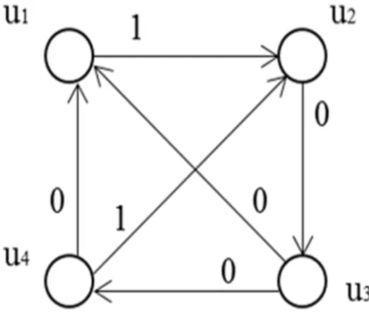
mutual testing is graph model (testing graph). Example of testing graph is shown in 90
Fig.2. 91
Figure 2. Example of testing graph
92
In the given case, diagnosable system consists of four units U={ u1, u2, u3, u4 }.
93
Each unit ui, ui∈ U, is assigned a particular subset of units in U to test.
Generally, a unit can test itself. Although, we assume that a unit doesn’t do this. 95
In the corresponding testing graph, it means the absence of loops (i.e., testing graph 96
doesn’t contain the edges that connect a vertex to itself). 97
A test, which invokes two units, is represented in the testing graph by the edge 98
between two vertices which correspond to testing and tested units. In Fig. 2, there 99
are six edges. These edges correspond to tests 12, 23, 34, 41, 31 and 42. Subscripts
100
point to the units that are involved in the test. The complete collection of tests is 101
called a testing assignment. Test result is represented by binary variable rij which
102
can take values 0 or 1. Variable rij is equal to 0 if unit ui evaluates unit uj as fault-free.
103
Otherwise, rij=1.
104
In Fig. 2, test results are shown next to the corresponding edges. The set of test 105
results is called a syndrome. Identification of faulty units using a syndrome is called 106
diagnosis. 107
Generally, for providing diagnosis at system level some assumptions are made, 108
such as: 109
tests can be performed only in the periods of time when system units do not 110
perform their proper system functions (i.e., when they are in idle state). That 111
is, a system unit is not tested continuously, and, therefore, there exists a 112
probability of not detecting the failed unit; 113
even if a unit is failed, a test not always detects this event. It depends on test 114
coverage; 115
result of a test is expressed as 0 or 1 depending on the evaluation of the 116
testing unit about the state of the tested unit; 117
tests in a system can be performed either according to a predefined testing 118
assignment or randomly. 119
In this paper, we consider that test coverage is equal to 100%. We also assume 120
that tests among system units are performed according to predefined testing 121
assignment. It means that the total time of testing is known beforehand. 122
Consequently, the periods of time when each unit is involved in tests are also known 123
in advance. 124
In the given case, it is possible to consider parameters of intermittent fault 125
model (i.e., and ) in relation to the total time of testing, ttesting. Table 1 presents
126
possible evaluations of values 1/ and 1/ as compared to the value of ttesting . This
127
comparison bears some resemblance to the techniques based on fuzzy logic. We 128
evaluate the values of 1/ and 1/ as “large” and “small” depending on the ratios 129
of values 1/ (1/) and ttesting .
130
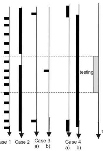
Table 1. Various types of intermittent faults
131
Ratio ttesting /A A=1/ A=1/
case 1 (class 1) large large
case 2 (class 2) large small
case 3 (class 3) small large
case 4 (class 4) small small
Figure 3. Different behaviors of intermittent faults
133
As a result of this consideration, it is possible to divide the considered 134
intermittent faults into several classes. 135
Intermittent faults related to class 1 and class 2 can be detected with high 136
probability during testing procedure. Detection of intermittent faults in case 3 is very 137
improbable (problematic). Probability of detecting such faults is low. As concerns 138
case 4, there exist two options – a) and b) (see Fig. 3). In the given case, probability 139
of intermittent fault detection can be estimated as 0.5 when 1/ 1/. 140
Generally, system level self-diagnosis is aimed at detecting permanently faulty 141
system units. Nevertheless, there exist the possibility to detect also intermittently 142
faulty units when intermittent faults are related to classes 1,2 and 4. 143
3.Problems with developing diagnosis algorithms when intermittent faults are 144
allowed 145
Diagnosis is performed on the basis of obtained syndrome. A syndrome is a 146
set of test results. The result of test ij is denoted as rij and can take the values 0 or 1
147
depending on the fact of how unit ui evaluates the state of unit uj.
148
In the paper, we accept the evaluation proposed by Preparata [ 17 ]. 149
0 if units u and u are fault-free
1 if units u is fault-free and and u is faulty
0,1 . when unit u is faulty
ij i j
i j
i
r =
X
150
We also assume that if an intermittent fault is in active state, then unit with this 151
fault behaves as permanently faulty unit. 152
To explain the problems with diagnosis made on the basis of obtained 153
syndrome, let us consider a simple example with code in Julia programming 154
illustration of how bitwise operations can effectively represent the operations on 156
syndrome. 157
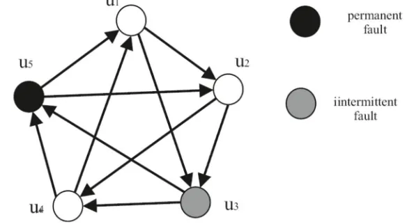
Let system consists of five units and tests are performed according to a 158
predefined schedule. This system is represented by graph shown in Fig. 4. 159
Obtained syndrome is 160
12 13 23 24 0 34 1 35 0 45 1 41 0 51 0 52 0
Rd= r{ =0,r =0,r =1,r ,r ,r , r ,r , r ,r } 161
Figure 4. Testing graph for the considered system
162
There exist several methods for diagnosis of permanently faulty units [20], 163
[21]. Most of them make the assumption about maximum possible number of faulty 164
units in the system. In [17], there was proved that correct system diagnosis is 165
possible if the total number of faulty units do not exceed the value t, where 166
1 2
N t
(2)
It is easy to verify that no system state (i.e., no combination of permanently 167
faulty and fault-free units in which the total number of permanently faulty units 168
doesn’t exceed the value t) can lead to obtaining such syndrome Rd. 169
For example, if units u3 and u5 are permanently faulty, result r13 should be equal
170
to 1, whereas in syndrome Rd this result is equal to 0. 171
Thus, direct application of algorithms developed for diagnosis only 172
permanently faulty units is not possible. 173
Such situation can be explained by specific behavior of some faulty units. 174
Particularly, a unit can be intermittently faulty. It means that at one moment it 175
behaves like a permanently faulty unit, whereas at other moments like a fault-free 176
unit. 177
Thus, new methods for diagnosis intermittently faulty units at system level 178
should be developed. 179
Testing graph of system can be represented by square adjacency matrix of 180
dimension NN, where N is the total number of units in the system. Elements of
181
this matrix are Boolean values. ( If unit ui performs test on unit uj , the item on i-th
182
row and j-th column takes the value true, otherwise false). Matrix of boolean values 183
can be represented in packed form. In the given case, matrix items are represented 184
Julia language supports bit arrays with arbitrary dimension by using standard 186
library of data structures.. Therefore the definition of new data type for data of 187
adjacency matrix is straightforward. 188
struct TestingGraph # testing graph 189
#is structure 190
tests::BitArray{2} # encapsulating 191
#two-dimensional 192
#bit array 193
end 194
Julia supports the definition of function which is performed on a new data type: 195
# constructor of new testing graph
196
# n = number of units
197
# test = specification of tests in
198
# form of vector of tuples
199
function TestingGraph(n::Int, tests::Vector{Tuple{Int, Int}})
200
tg = TestingGraph(falses(n,n))
201
for (checking, checked) in tests
202
tg.tests[checking, checked]=true
203
end
204
return tg
205
end
206
#auxiliary function(returns number of units)
207
size(tg::TestingGraph)=size(tg.tests,1)
208
209
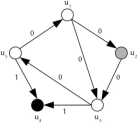
Usually a syndrome is depicted in testing graph as weights of edges. In the given 210
case, weights are results of tests. A result can take values either 0 or 1. In Fig. 5, 211
example of syndrome for the system with five units is shown. 212
Figure 5. Instance of syndrome for the testing graph
213
This type of weighted graphs can be represented by a pair of Boolean matrices 214
(in packed bit array representation). The first matrix (denoted as mask) is identical 215
to adjacency matrix of testing graph it defines the positions of valid results (i.e., 216
results equal to 0). The second matrix codes results of tests (true represents result 217
equal to 0, false represents result equal to 1). Only results with true bit in the mask 218
Definition of syndrome representation in Julia language with basic constructor 220
is shown below. In the given case, results are specified as tuples of indexes of testing 221
and tested units and numerical representation of test result. 222
223
struct Syndrome 224
mask:: BitArray{2} 225
results::BitArray{2} 226
end 227
function Syndrome(n::Int, results:: Vector{Tuple{Tuple{Int, Int}, 228
Int}}) 229
# both matrices are inicialized by falses 230
s = Syndrome(falses(n,n), falses(n,n)) 231
s.results[checking, checked] = (result == 0) # set bit in results 232
s.mask[checking,checked]=true #and mask 233
end 234
return s 235
end 236
237
For example the syndrome depicted in Figure 5 can be created by this call of the 238
constructor: 239
R_d = Syndrome(5, [((1,2), 0), ((1,3),0), ((2,3), 0),((3,4), 1), ((3,5), 240
0), ((5,1), 0), ((5,4), 1)]) 241
If we assume that in the considered example units u2 and u4 are permanently
242
faulty, then the set of all potential syndromes will be obtained. This set R contains 243
two syndromes and can be defined as follows 244
12 0 13 0 23 34 1 35 0 51 0 54 1 0 1 { , , , , , , }, where X ,
R u u u X r u u u
245
Checking if syndrome is a member off set R for the system with faulty units in 246
Julia is simple and effective. Such checking is based on the standard bitwise 247
operations AND, XOR and OR. The set of syndromes is expressed by standard 248
syndrome structure with slightly alternative meaning of bit mask. In the given case, 249
true bit in mask is interpreted as unambiguous result of test. False bit is interpreted 250
as ambiguous result of test (in set R, it is denoted as "X") or non-existent test. 251
252
# syndrome membership in syndrome set #(s is element of s_set)
253
function ∈(s::Syndrome, s_set::Syndrome) 254
if s_set.mask .& s.mask != s_set.mask 255
throw(ArgumentError("Incompatible syndrome")) 256
end 257
cover=(s_set.results.⊻s.results).& s_set.mask 258
return !reduce(|, cover) 259
end 260
The main part of checking if syndrome is a member of set R exploits the map-262
reduce approach. Here, XOR is applied between bit array of results of obtained 263
syndrome and bit array of expected results of syndrome. Operation is performed 264
only on valid bits of set R (see mask operation by AND). Reduce step is performed 265
by bitwise OR (any true bit leads to denial of membership). 266
267
# creation of syndrome set for given test # graph `dg` 268
# and boolean array of units states #(false = faulty units)
269
possible_syndrome_set(tg::TestingGraph, 270
unit_states::BitArray{1}) 271
= Syndrome(tg.tests.&unit_states, tg.tests .& 272
unit_states') 273
274
The mask array of set R is constructed by vector application of bitwise AND 275
between adjacency matrix of testing graph and column vector of unit’s states. That 276
is, operation AND is applied on rows (because validity of testing is determined by 277
testing unit. The result array of set R is outcome of application of transposed vector 278
of unit’s states and adjacency matrix (operation AND is applied on columns because 279
results of testing are determined by tested unit). 280
281
Checking if syndrome R_d is a member of R for system with two faulty units is 282
obvious 283
284
R_d ∈ possible_syndrome_set(tg, BitArray([true, false, 285
true, false, true]) 286
As can be seen, the syndrome R_d does not belong to the set R since any 287
syndrome that belongs to R has r12 equal to 1, whereas in the syndrome R_d this
288
result is equal to 0. 289
It can be explained by the fact that unit u2 has an intermittent fault which
290
transfers from AS (PS) to PS (AS) during testing procedure. In view of this, most of 291
the algorithms developed for diagnosis of permanently faulty units cannot be 292
directly used for diagnosis intermittently faulty units. 293
Nevertheless, there was suggested the method [10] based on summary 294
(updated) syndrome, . Summary syndrome is obtained after performing m 295
rounds of test routine (i.e., m repetition of tests). Summary syndrome is 296
computed as follows: 297
lrij Σ ij ij
l
R = r , r = , (3)
where l ij l
r R , Rl -syndrome obtained in l -th round of repetition of test routine. 298
The summary syndrome is computable by reduction of syndrome list by binary 299
operation of syndrome union. This operation is implemented by bitwise AND 300
between result bit array of syndrome (result 1 is represented as false!). 301
302
if s1.mask != s2.mask 304
throw(ArgumentError("Incompatible syndromes")) 305
end 306
return Syndrome(s1.mask, s1.results & s2.results) 307
end 308
R_all = reduce(, list_of_syndromes) 309
310
When summary syndrome R
is a subset of set R0 (i.e., R R0), the algorithms
311
developed for diagnosing permanently faulty units can be also used for considered 312
faulty situation. R0 is a set of syndromes that can be obtained when only
313
permanently faulty units can take place (considering that real number of faulty units 314
do not exceed the maximum number of faulty units which is allowable for 315
diagnosable system). The set R0 is constructible by mapping of function
316
possible_syndrome_set over iterator all possible permutation of states of units in 317
diagnosable system (bit arrays of all permutations of unit’s states are obtained from 318
binary numbers between 0 and 2n). 319
320
function iter_possible_states(tg::TestingGraph)
321
n = size(tg)
322
t = (n-1)÷ 2 # integer divison
323
return (set for set in
324
(BitArray(digits(i, base=2, pad=n)) for i=2^n-1:-1:0)
325
if n-count(set) <= t) # only with maximal t faulty
326
end
327 328
In the given case, the task arises to determine the number of test routine 329
repetitions, l. Neither is determined what should be done if after l repetitions the 330
condition RΣR0is not true.
331
To solve these tasks, we suggest the following decision. It is suggested to repeat 332
the test routine several times, l. Concrete number of repetitions of test routine
333
depends on the total number of units in the system N, on the classes of intermittent 334
faults, which are going to be detected, and on the required credibility of diagnosis. 335
If an intermittent fault belongs to class 4, the value of l does not influence the test
336
results. If an intermittent fault belongs to class 3, a unit with such fault behaves either 337
as fault-free or as faulty only during one test. Any next test will show that this unit 338
behaves as fault-free. Thus, two test are sufficient to form rij which make condition 339
R R0 true. It also concerns an intermittent fault of class l. In case 2, a unit with
340
such intermittent fault with high probability will behave as permanently faulty. 341
There is low probability that one of the tests will show that this unit is fault-free. 342
Although, any other test will show that this unit is faulty. Thus, two tests are enough 343
to form Rwhich satisfies the above mentioned condition.
344
If after several rounds of tests repetitions the condition RΣR0 is not true, then
345
that, according to the summary syndrome, are diagnosed as fault-free. Units that 347
belong to the set evaluate each other as fault-free. In order to determine the set 348
u
K , it is needed to remove from summary syndrome RΣ all test results which are 349
equal to 1. Remaining results allow to form a Z-graph. 350
Z-graph is formed as follows. If rij in RΣ is equal to 0, then there is an edge 351
between vertices vi and vjin Z-graph directed from vi to vj . 352
Credibility of diagnosis result will be greater when Z-graph is connected [15]. In 353
Fig. 6, examples for connected and disconnected Z-graphs are shown. 354
355
a) Z-graph is disconnected b) Z-graph is connected
Figure 6 . Examples of Z-graph
Connection of Z-graph depends considerably on testing assignment and on the 356
allowed number of faulty units (i.e., on the maximum number of faulty units that 357
still allows to obtain the correct result of diagnosis). 358
We consider the case when tests among system units are performed in 359
accordance with a pre-set schedule (i.e., defined a priori). Having the testing graph, 360
it is possible to investigate if Z-graph is connected under the condition that 361
maximum number of faulty units doesn’t exceed value t. 362
Since each edge of graph involves two vertices, the minimal number of edges 363
which still allows to provide system t-diagnosability [7], Lmin, is equal to 364
min
( 1)
2
N t +
L =
(4) Next, we can examine if the value Lmin is sufficient in order that Z-graph be
365
connected. 366
Given Lmin, we can determine the minimal number of edges in Z-graph, Kmin, that
367
ensures connection among its vertices. Kmin can be determined as follows
368
min
( 1)
2
t +
K =
( 5 )
Z-graph is connected if 369
1 2 1 2
2 min
t t
K or t t (6)
This inequality is true for t < 3 (that is, when total number of system units is less 370
In case when N ≥ 7, value Lmin is not sufficient in order that Z-graph be connected.
372
In the given case, we can determine the number of additional edges that must be 373
added to Z-graph in order that this graph becomes connected. 374
Using results presented in [15], it is possible to conclude that Z-graph maximally 375
may have 376
( )
2
N t
π =
(7)
components each of which consists either of two vertices for N 3 4a a, 0 1 2, , ,, or
377
of two vertices except the one consisting of three vertices for N 5 4a a, 0 1 2, , , 378
In order to connect these π components (π-1) additional edges are necessary. 379
The choice of the pair of units for performing a test that corresponds to the additional 380
edge in Z-graph can be carried out according to existing algorithms [15]. 381
For Z-graph it is possible to form the matrix MR. Matrix MR is square matrix
382
presentation of the subset of RΣ which has only zero results. If result rij is an element 383
of the resulting subset of RΣ , then element mij of matrix MR has value of 0. 384
Otherwise, element mij is denoted as dash. 385
There could be used the diagnosis algorithm presented in [9]. This algorithm is 386
based on the matrix which is similar to matrix MR and can identify all faulty units 387
(on the condition that total number of faulty units does not exceed the value t ). 388
Handling matrices like MR is also presented in [3], [5]. 389
In the given case, it is needed to calculate the total number of 0 in each column. 390
Then, obtained numbers S , i =i 1, N, should be compared with value t. If Si t, then 391
unit ui1
n is diagnosed as fault-free. If condition ≥ is not true for all ∈ {1, … ,N}
392
then it is needed to find in Z-graph a simple directed cycle of length t +1. Such cycle
393
can be determined from matrix MR . All units, which are in this cycle, should be 394
identified as fault-free. 395
Units that are not identified as fault-free are either permanently faulty or have 396
an intermittent fault. It should be noted that there is low probability of incorrect 397
diagnosis. This probability can be evaluated in relation to different total number of 398
system units, different classes of intermittent faults and different number of test 399
routine repetitions. 400
4. Conclusions 401
Mostly, system level self-diagnosis deals with the diagnosis of permanently 402
faulty units. Although, there are many real situations when intermittently faulty 403
units can occur in the system. In the given case it is necessary to take into account 404
various behaviors of such faulty units. 405
Behavior of intermittent fault can be modeled by continuous Markov chain with 406
two states – Passive (PS) and Active (AS). If an intermittent fault is in PS, unit acts 407
as fault-free. If an intermittent fault is in AS, unit acts as fault (i.e., as if it has a 408
During system level self-diagnosis both permanent and intermittent faults can 410
occur. Each test evaluates the state of a unit either as fault-free or as faulty. In the 411
latter case, it does not discriminate the permanent and intermittent faults. 412
Diagnosis algorithms that deal with the sets of test results can consider (take into 413
account) the testing time and, thus, potentially they could discriminate the 414
permanent and intermittent faults. For this, the testing procedure must be very long. 415
In reality, it is needed to perform the testing procedure in acceptable time for each 416
concrete system. This leads to the situation when it is very difficult to discriminate 417
between permanent and intermittent faults. In view of this, suggested diagnosis 418
algorithm can identify only fault-free system units. All units that are not diagnosed 419
as fault-free should be considered as faulty without further specification. 420
Suggested diagnosis is developed on the basis of consistent sets of system units. 421
Units that belong to consistent set with high probability can be considered as fault-422
free. When situation allows to extend the testing time, it is possible to gain higher 423
probability that units of a consistent set are fault-free. 424
Author Contributions: Viktor Mashkov wrote the theoretical part of the paper 425
Jiří Fišer developed the algorithms in Julia language Volodymyr Lytvynenko 426
contributed to theoretical part and developing the codes Maria Voronenko 427
prepared and formed the manuscript 428
429
References 430
1. A. Avizienis, J.C. Laprie, B. Randell.Fundamental concepts of dependability. Technical Report Series 431
University of Newcastle upon Tyne, Computing Science 1145 (010028), 2001, pp. 7-12. 432
2. A. Avizienis, J.C. Laprie, B. Randell. Dependability and its threats. A Taxonomy. IFIP 18th World Computer 433
Congress “Building the Information Society”, France, 2004, pp.91-120. 434
3. S. Babichev, V. Lytvynenko, M. Korobchynskyi, M. A. Taif. Objective clustering inductive technology of 435
gene expression sequences features. Communications in Computer and Information Science, 2017, pp.359-372. 436
4. G. Hetherington, et. al. Logic BIST for large industrial design: real issues and case studies. ITC, 1999. 437
5. S. Babichev, M. A. Taif, V. Lytvynenko, V. Osypenko. Criterial analysis of gene-expression sequences to 438
create the objective clustering inductive technology, Proc. of IEEE 37th International Conference on Electronics 439
and Nanotechnology, ELNANO, 2017, pp. 244-248. 440
6. Mashkov supervised of the project 441
7. S. Kamal, C. V. Page. Intermittent fault: a model and a detection procedure. IEEE Trans. Comput. Vol.C-23, 442
No.7, 1974. pp.713-719. 443
8. L.E. Laforge, K. Huang, V.K. Agarwal. Almost sure diagnosis of almost every good elements.IEEE Trans. 444
on Computers, Vol.43, No.3, 1994, pp. 295-305. 445
9. [8] P. Maestrini, P. Santi. Self-diagnosis of processor arrays using a comparison model. In Proc. Of 14th IEEE 446
Symposium on Reliable Distributed Systems, 1995, pp. 218-228. 447
10. V. Mashkov. Selected problems of system level self-diagnosis. Lviv: Ukrainian Academic Press, 2011, 184 448
pages. 449
11. S. Mallela, G. Masson, Diagnosable systems for intermittent faults. IEEE Trans. Comput., Vol.C-27, No.6, 450
1978. pp.560-566. 451
12. [11] V. Mashkov. Task Allocation among Agents of Restricted Alliance. Proc. of IASTED ISC’2005 conference, 452
pp. 13-18, Cambridge, MA, USA, 2005. 453
13. V. Mashkov, J. Barilla, P. Simr. Applying Petri Nets to Modeling of Many-Core Processor Self-Testing when 454
Tests are Performed Randomly, Springer, Journal of Testing, 2013, DOI: 10.1007/s10836-012-5346-8. 455
14. V.A. Mashkov, O. V. Barabash Self-testing of multimodule systems based on optimal check-connection 456
15. V.A. Mashkov, O. V. Barabash Self-checking of modular systems under random performance of elementary 458
checks // Engineering Simulation, 1995, Vol. 12, pp. 433-445 459
16. V. Mashkov, J. Pokorny. Scheme for comparing results of diverse software versions. In Proc. of ICSOFT 460
Conference. Barcelona, Spai, 2007, pp. 341-344. 461
17. J.C. Laprie, editor. Dpendability: Basic Concepts and Terminology. Springer-Werlag, 1992. 462
18. T. Preparata, G. Metze, R. Chien. On the connection assignment problem of diagnosable system. IEEE 463
Trans. on Electronic Computers, Vol. EC-16, No. 12, 1967, pp. 848-854. 464
19. M. Psarakis, D. Gizopoulos, E. Sanchez, M. Sonza Reorda. Microprocessor Software-Based Self-Testing. 465
IEEE Design & Test of Computers, Vol.27, No.3, 2010, pp. 4-19. 466
20. S. Su, I. Koren,.K. Malaiya. A continuous-parameter Markov model and detection procedures for 467
intermittent faults. IEEE Trans. Comput. Vol.C-27, No.6, 1978. pp.567-570 468
21. G. Sullivan. An O (t3 + E ) fault identification algorithm for diagnosable systems. IEEE Trans. Comput., Vol.
469
C-37, 1988, pp. 388-397. 470
22. V. Vedeshenkov. On organization of self-diagnosable digital systems. Automation and Computer Engineering, 471
Vol. 7, 1983, pp. 133-137. 472
23. H. Fujiwara, K. Kinoshita. Some existence theorems for probabilistically diagnosable systems. IEEE Trans. 473