Controlling processes with reference to costs, item price and process evolution

CONTROLLING PROCESSES

WITH REFERENCE TO COSTS,

ITEM PRICE AND PROCESS

EVOLUTION

Violetta Iwona Misiorek

A thesis submitted in fulfillment of the requirements for the

Master of Science Degree

School of Communications and Informatics

Faculty of Engineering and Science Victoria University

"Necessity to study the needs of the customer, and to provide

service to product, was one of the main doctrines of quality taught

to Japanese management in 1950, and onward"

W. Edward Deming

"Quality, Productivity and Competitive Position", 1982

"A dissatisfied customer does not complain: he just switches"

CONTENTS

Page

DECLARATION i

ACKNOWLEDGEMNTS ii

ABSTRACT iii

CHAPTER 1. Introduction

1.1 Origins of quality control 2

1.2 Design of control charts 3

1.3 Changes in process m e a n 4

1.4 Thesis objectives 5

CHAPTER 2. Literature Review

2.1 Introduction 8

2.2 Selection of the process m e a n 8

2.2.1 Standard process 8

2.2.2 Selection of the process m e a n under a

sampling plan 11

2.2.3 Simultaneous selection of a variable and an

attribute process m e a n 12

2.2.4 Selection of the process m e a n with special

reference to a canning problem 12

2.3 Processes with a trend or shift in m e a n 14

maximization of profit 18

2.3.1.4 Non-linear systematic and random

shifts in m e a n 19

2.3.2 Controlling processes with m e a n trend 21

2.4 Shifts in process variance 22

2.5 Conclusion 23

CHAPTER 3. Factors Affecting the Choice of

Target

3.1 Introduction 26

3.2 Factors affecting the choice of target for processes

with 'top-up' and 'give-away' 28

3.2.1 Methodology 28

3.2.2 Theoretical analysis 30

3.2.3 Dependencies between the process parameters 31

3.3. Concluding remarks 43

CHAPTER 4. Mean Selection for a Filling Process

4.1 Introduction 45

4.2 General problem 46

4.3 Theoretical analysis 48

4.3.1 Finite capacity containers 48

4.3.1.1 Model 1 48

4.3.1.2 Model 2 54

4.3.2 W h e n overflow is not an issue 60

4.3.2.1 Model 3 60

4.3.2.2 Model 4 63

4.3.2.3 Model 5 64

4.4 Modelling processes with additional costs 68

4.5 Infinite and finite capacity containers - comparison 72

4.6 Concluding remarks 7 4

CHAPTER 5. Weights and Measures Requirements

5.1 Introduction 76

5.2 Australian requirements and the probability of not

breaching the legislation 76

5.3 O I M L international recommendations 79

5.3.1 Statistical tests-general rules 79

5.3.2 Sampling plans-recommended examples 81

5.4 Regulations in selected countries - comparison with australian

requirements 83

5.5 Conclusion 92

CHAPTER 6. Industrial Example

6.1 Introduction 95

6.2 Example- Laundry powder manufacturing 95

6.2.1 S o m e dependencies between process parameters 96

6.2.2 Graphical solution 97

6.2.3 Numerical solution and implications to weights

and measures requirements 98

6.2.3.1 Implications to other countries

requirements 103

6.3 Concluding remarks 106

7.3 Dependencies between process parameters 112

7.3.1 E[P(x)] against initial process setting 112

7.3.2 Trends in standard deviation 113

7.3.3 Changes in shift size of the m e a n 116

7.4 Concluding remarks 118

CHAPTER 8. Conclusion and Suggestions for

Future Work

8.1 S u m m a r y and conclusion 120

8.2 S o m e suggestions for future work 121

APPENDIX 124

DECLARATION

I hereby declare that:

(i) the following thesis contains only original work which has not

been submitted previously, in whole or in part, in respect of any

other academic award, and

(ii) due acknowledgment has been made in the text of the thesis to

all other material used.

ACKNOWLEDGEMENTS

I would like to express m y gratitude for the guidance, support and help offered

by my supervisor, Associate Professor Neil S. Barnett, during my period as a research student at Victoria University. He has provided many ideas as well as invaluable suggestions and comments on many aspects of this thesis.

Special thanks are due to all the staff and research students of the former Department of Computer and Mathematical Sciences, Victoria University, for their

assistance and for making my time at the University so enjoyable. In particular I wish to acknowledge the assistance of Dr. Neil Diamond with the S-Plus code for

approximation of equation (5.1). His friendly advice, helpfulness and encouragement are much appreciated. I am grateful also to my co-supervisor, Associate Professor Peter Cerone, for his many useful remarks and suggestions.

I am thankful to CSfRO, Mathematical and Information Sciences, for their

support in the final stages of this research. Special thanks are due to Dr. John Field for his permission to use his method for calculating the probability of failing the weights and measures requirements in EEC and USA. This assistance is gratefully

acknowledged.

Finally, I wish to extend my most sincere thanks to my husband Piotr and my children, Gabriella and Piotr S., for their understanding, love and patience. A special credit is owed to my mother for her help during this work.

The research for this thesis was supported by a Department of Computer and Mathematical Sciences studentship. This assistance is gratefully acknowledged.

ABSTRACT

This thesis presents some recent work of the author in developing the analysis

of a number of process control models that take into account statistical, economic and other practical issues. Special attention is paid to the problem of optimum selection of the initial process mean setting, with particular reference to filling/canning processes. As there are many different situations that involve different cost parameters, this leads to the consideration of various models each with their own particular solution. The

effects of change of the process variance on the optimal solution as well as on the expected profit are discussed. Implications to 'Weights and Measures' requirements of following this optimality path are provided, with particular reference to loss in expected profit per item.

Chapter 1 provides a brief introduction and is followed by a literature review in Chapter 2.

Chapter 3 deals with the issue of selecting the optimum process mean by

presenting a simple model and emphasising the dependencies between the process parameters.

Chapter 4 further investigates the problem presented in Chapter 3 and presents several models for which the selection of the most profitable process setting is considered, concentrating on a canning problem. Various industrial filling processes are described and some of the issues considered include: waste, overfill, top-up, and the penalty costs for items that initially fail to meet specifications.

recommendations are discussed. T h e Australian requirements are also compared with the requirements of the European Economic Community as well as the United States. Chapter 6 illustrates the potential use of the models developed in chapter 4 by giving an industrial example and again discussing the implications to Weights and Measures requirements.

In Chapter 7 the problem of an optimal selection of the initial process mean is

examined for a process with a linear shift. Special focus is on the economic benefits obtained from reducing process standard deviation and the rate of change of the mean. Conclusions and some suggestions for future work are provided in chapter 8.

Parts of chapter 4, 5 and 6 form the contents of a paper, 'Mean Selection for Various Types of Filling Process with Implications to 'Weights and Measures' Requirements', undergoing revision for publication in the Journal of Quality Technology.

CHAPTER 1

1.1 Origins of quality control

The origin of modern industrial quality control dates from May, 1924 when a young, Walter Shewhart, developed the first sketch of a process control chart. Shewhart was born on March 18, 1891 and received his Ph.D. in physics from

the University of California in 1917. He worked with the Western Electric Company

before joining Bell Laboratories in 1925. It was there that his ideas regarding application of statistical methods to the analysis of physical and engineering data started to

stimulate the interest of other scientists. His methods became more and more accepted, boosted by the presentation of his paper on the economic control of quality of

manufactured product to the Royal Statistical Society, in 1931.

Shewhart was the first to prescribe methods by which a process could be gauged

to have reached a state of statistical control. Statistical methods for quality control have been widely used since then, being elevated in importance by the post war industrial

success of Japan. Many western countries were too complacent, and totally unaware of the industrial competition they were shortly to face with the dramatic effects this would have, to have had an intimate interest in the industrial application of statistics. Deming and Juran contemporaries of Shewhart, became strong advocates of the use of statistical techniques in the industrial environment in order to assist efforts of process control and improvement of product quality. Deming, in particular, espoused such techniques to the Japanese who claim a strong connection between this and their climb to industrial

prominence from the ashes of destruction of 1945. Statistical methods in quality control are now widely accepted throughout the world, as they are adapted to suit advancing technology.

Statistical Process Control ( S P C ) is a statistical approach to production that is

used to ensure that processes are maintained in a state of statistical control. Such control helps to ensure that manufactured products are consistent in their vital parameters,

although, of course, all processes are subject to a certain amount of variability. Walter Shewhart made the distinction between common and special causes of variation. The

latter are often referred to as assignable causes and the former, which are considered solely due to chance, are called common (random) causes. Any random cause results in process and product variation but generally such causes cannot be economically

eliminated. Assignable variation, however, is assumed to be due to specific "findable" causes and action to eliminate these is usually economically justifiable. Ideally, only random causes should be present in a process. Control charts, which were invented by Shewhart, are often used to distinguish between assignable and random causes and for prompting process adjustment.

1.2 Design of control charts

There are two basic approaches to designing control charts, economic design and

statistical design. Economic design is a method of selecting the design parameters in such a way as to either minimise the total cost of production or to maximise the producer's profit. The method requires the assessment of several cost and non-cost

been published in the area of economic design of control charts up until then. This w a s followed by Ho and Case (1994) who reviewed the literature for the years 1980-1991. As has been indicated by several authors, the economic method of designing

control charts has certain weaknesses. One of the main drawbacks in the use of

economic models is their poor statistical performance (e.g. insensitivity to small shifts in process parameters). In addition, total cost savings, that economic designs are supposed to yield, frequently do not accurately reflect reality, Woodall (1986). As Woodall

(1986b) has shown, economic models generally do not agree with Deming's (1982)

philosophy, which states that the main focus of process studies should be on improving the process.

A common assumption made when examining economic aspects of quality

control is that the most desirable values of the process parameters are known and that the task is to optimize procedures for controlling the quality. The methods of quality control should not be applied to the process until the most economic values of the process parameters are selected. The role of process control methods should then be to ensure that the selected values of the parameters are achieved.

1.3 Changes in mean

The objective of any process control system is to make sound decisions on

actions to be taken that affect the process. A process is said to be operating in statistical control when the only sources of variation are common causes. Most statistical process

control (SPC) techniques assume that process data can be described in terms of

statistically independent observations that fluctuate about a constant mean. In reality, however, many manufacturing processes exhibit systematic trend in one or more of the

process parameters during the course of operation. This can often be linked to machine reliability. Such changes often occur in production processes that involve drilling, grinding or cutting (Taha (1966) as well as many others). This type of trend is often a consequence of tool-wear. The general approach of SPC is to establish stability (fixed mean and constant variability) and leave the process unadjusted whilst it produces items between certain established statistically desirable boundaries. The design of a process that manifests systematic trend, for example in its mean, requires first the selection of the initial setting of the mean level as well as some kind of control regime that would regularly require the process to be adjusted. Such an approach ignores the issue of assignable causes. With an economic approach what is required is the striking of a balance between different costs involved in the manufacturing process. Such costs

include the setup costs, production costs and the financial penalty of actually producing defective items. In SPC, a quantum "jump" in the mean is usually interpreted as an

assignable cause that needs to be rectified. If certain supplementary run rules are used in SPC charts these provide facility for detecting a trending mean but, generally, ensuing process adjustments are made on statistical rather than economic grounds.

1.4 Thesis objectives

The main thrust of this thesis is to present and bring together some of the work that has been published on SPC and economical design of control mechanisms.

expected profit. T h e need to consider whether or not the obtained results meet Australian 'Weights and Measures' requirements is also discussed. The method of

calculating the probabilities of meeting Legislation requirements is shown. Furthermore, OIML (The Organisation Internationale de Metrologie Legale) International

Recommendations are described and the Australian requirements compared with other selected countries' Legislation.

In addition, a model, which is applicable to a process that exhibits a linear shift in mean, is presented.

The dependencies between process parameters are analysed in detail and

displayed graphically. An industrial example is also given as an illustration of the methods proposed.

Once the selection of the optimal process parameters is complete a brief

summary of statistical methods used to maintained the current process state is given. Chapter 2 presents a review of the published work on the economics of process

settings and adjustment when there are systematic changes in the process mean and / or variance.

CHAPTER 2

2.1. Introduction

The economic design of control charts has been the focus of a considerable

amount of work during the last forty years. Comparatively little has appeared,

however, on the economic selection of the parameters especially in relation to filling

processes. Models that apply to processes that exhibit shift in mean or variance,

although being discussed by many authors, consider mainly processes involving

cutting, griding rather than filling processes.

This chapter gives a review of models and techniques proposed for selecting

the most desirable quality characteristic with special attention given to canning

problems. This is followed by a review of work published on controlling processes

with an inherent shift in mean or variance.

2.2 Selection of the process mean

2.2.1 Selection of a process mean for a standard process

Pioneering work in the area of optimum setting of the initial process mean was

published by Burr (1949) , Springer (1951) and Bettes (1962). They all considered

related problems; the latter two took economic aspects into account and determined

the optimal location of the mean, which minimises the total cost. The work of

Springer was later extended by Nelson (1979).

Most work published on economic design concentrates on minimising the

costs of production. This works well only for a simple pricing policy, i.e. if the

product meets the specified requirements then it's sold at a regular price, if it does not

then it is considered scrap. In reality, however, even if the product does not meet the

specifications it may still be sold at a reduced price. In this situation the minimisation

of the production costs could cause diminution in quality. W h a t is more, the overall goal for most modern production processes is to manufacture with a "quality" that maximises total profit. Hunter and Kartha (1977) developed a method for determining the optimal target value of an industrial process so as to maximise the profit, taking process variability and production costs into account. The problem revolves around the situation where product above a certain dimensional threshold attracts a fixed

selling price and product below the threshold attracts a reduced yet fixed selling price. In addition, product above the threshold implies 'give-away' which diminishes the net profit per item. The essential issue is to find the most suitable process setting ( the process mean) so as to effectively trade off diminished profit due to 'give-away' with diminished profit induced by producing below the stipulated threshold. Besides

successfully formulating the problem, Hunter and Kartha provide a graphical method of solution. The authors consider the problem under the assumption that once the initial setting is made, no other control actions are subsequently required. The assumed conditions in their model do not permit for an explicit optimal solution, however Nelson (1978) has found an approximating function which allows for about three-decimal accuracy in the solution. He has also included a plot of errors of this approximation.

nominal weight or volume cannot be sold. A solution for a process having an approximate normal distribution was given together with a table that provides a

simple way of getting the optimal process setting. Situations in which the distribution of the quality characteristic has lognormal and Poisson distributions were also

discussed. The objective was to maximise the profit. Vidal (1988) has later examined this problem in more detail and given a mathematical discussion of the optimisation model. He explored the properties of the optimisation model, its stationary solution, found by a graphical method, and also gave examples of some special cases where the stationary points can easily be found. The proposed methods, however, were

dependent on the assumption that the prices and costs are linear functions of the quality characteristic.

A model also similar to that of Hunter and Kartha was studied by Carlsson

(1984). He analysed the choice of the process setting as well as the net expected

income taking production costs, selling price, process variability, specification levels, and control plan all into account. An example from the steel construction industry, where rejects are either sold at a reduced price or reprocessed was given. The quality characteristic was assumed to be one-dimensional and normally distributed with

known variance. Furthermore, one specification level, defined as the lower level, was assumed and the net income function was represented as a piecewise linear function of the quality characteristic. The situations where a customer is willing to pay extra for good quality as well as when a producer may have to compensate the customer for bad quality, are both discussed.

2.2.2 Selection of the process m e a n u n d e r a sampling plan.

All of the studies discussed so far, have addressed the problem of quality selection assuming 100% inspection of product. Carlsson (1989) and Boucher and Jafari (1991) have extended this line of research by evaluating the problem under a sampling plan.

Carlsson (1989) considered a case of acceptance sampling where the reject

criterion was based on the sample mean. Special attention is given to the MIL-STD-414 acceptance sampling plan. He assumed just one specification limit, given as the lower limit, and that the quality characteristic follows a normal distribution with known variance. The rejected lot is sold at a secondary market or reprocessed. The expected income function proposed is similar to that of Carlsson (1984). As the solution is not explicitly obtainable an approximation is given. He noted that the approximation accuracy improves as the sample size increases.

Boucher and Jafari (1991) considered the case in which the rejection criterion is based on the number of nonconforming units in the sample. Special attention is

given to a filling process where it is not possible or economically justifiable to inspect every unit of product. They consider a sampling plan in which a sample of size n is

2.2.3 Simultaneous selection of a variables a n d a n attribute target m e a n

Some industrial processes involving paper, plastic, glass and fabric have to

satisfy both variables as well as attribute quality characteristics. The former of the two might correspond to weight or volume, hardness, or size, the latter usually relates to cracks, abrasions, and marks. Arcelus and Rahim (1994) discussed such cases. The

objective of the model developed was the maximisation of the expected profit. The variable quality characteristic was assumed to be normally distributed and to have a lower specification only, with the attribute quality characteristic being Poisson and having a single upper specification limit. The two quality characteristics were

assumed to be independent. The authors have adopted a Taguchi like loss function by penalising deviations from the target as well as excess of non-conformities. The optimal solution was found by using an iterative approach based upon the ZEROIN

routine of Forsythe, Malcolm and Moller (1977). For ease of computation the attribute characteristic was assumed to be modelled by a real-valued variable rather than a discrete variable.

2.2.4 Selection of the process mean with special reference to a canning

problem.

Operations that involve placing any ingredient into containers, be it fluid or

solid, are typical of the 'canning problem'. Models to be used for optimally setting the mean have to take into account not only the nature of the process but also different cost parameters.

T h e models developed by Hunter and Kartha (1977) as well as Bisgaard,

Hunter and Pollesen (1984) and discussed in the previous section, can also be applied to canning processes, however the assumptions they made for under-filled containers

are frequently unrealistic. It is in breach of the law to sell under-filled items for either reduced price or at a price proportional to the amount of ingredient in the container.

Some of the earliest work in the area was presented by Golhar (1987) who addressed the issue of finding the most economic setting of a process mean,

concentrating specifically on a canning problem. He modelled a situation where only correctly or overfilled product can be sold at a regular price and under-filled cans are emptied and refilled with added cost. The capacity of the containers was implicitly assumed infinite.

The canning problem analyzed by Gohlar was latter discussed by Schmidt and

Pfeifer (1989), who explored the cost reductions achievable through a reduction in the process standard deviation. A linear relationship between the percentage reduction in cost and process standard deviation was found. They also noted that the final

equations were independent of item price, as all containers are sold for the same amount. Revenue per can was constant thus minimization of expected cost is

equivalent to maximisation of expected profit.

Golhar later extended his model (Golhar & Pollock (1988)), for a process

where ingredients are expensive and where both the process mean and the upper limit can be controlled. The concavity of the solution function was shown only by a

A similar problem w a s discussed by Schmidt & Pfeifer (1991) and they have extended the above model to situations where a fixed capacity container was assumed. In both of the models discussed above the profit per fill attempt or item, P(X), (as defined by Schmidt & Pfeifer and Golhar & Pollock) was as follows:

If the item falls within specifications then

P(X)= Revenue per acceptable container - material cost

Otherwise it incurs a loss. No other variations of the profit function were discussed.

2.3. Processes with a trend or shift in mean

Many manufacturing processes exhibit some sort of trend in one or more of the

process parameters during the course of operation. Often this trend is of a systematic nature and its relationship with time is also frequently linear. Trends can be negative or positive. The former of these occurs ,for example, when the nozzle of a filling

machine is clogged, the latter is a characteristic of tool-wear. Such changes usually occur in production processes that involve drilling, grinding or cutting (Taha (1966) and others) as well as filling. The process is kept in control by regular adjustments, replacements of some parts of the tool or, in the case of nozzles, by cleaning.

2.3.1 O p t i m u m selection of the process m e a n

2.3.1.1 Linear shift in mean and tool-wear.

The first consideration of the effects of a linear trend on the process mean due to tool wear was made by Manuele (1945). His approach was subsequently

popularised by Duncan (1974), Vaughan (1974), and Grant and Leavenworth (1980). As the tool wears the average of the process increases. There is always a limit to how big the process average can get before the amount of defective items is

intolerable. On the other hand, resetting is usually quite expensive. A balance must be obtained between these two costs. The following summarises the literature describing methods for the optimal selection of the length of the process run.

Gibra (1967) considered the case of a process that was known to exhibit a

linear trend in the mean while having a constant variance. He obtained the optimal production run between process adjustments by controlling the initial setting of the mean for both stable and unstable processes. The case of statistical stability involved minimisation of the sum of the resetting cost and the financial loss due to

size, control limit width and the initial setting, could all be found. T h e solutions for both the single and two-sided specification cases were provided.

Taha (1966) also discussed the problem of tool-wear with special reference to

cutting tools. The assumption was made that any increase in the number of defective items was due to tool wear only. The overall objective of his work was to determine the optimal length of time before maintenance should occur. This requires minimising the sum of the reworking and/or scrapping costs of defective items and the cost of adjustments.

A slightly different and more general approach was demonstrated by Smith

and Vemuganti (1967). They assumed that the wear of the tool was a linear function

of time and that the distribution of the initial mean, as well as the rate of wear of the tool, is known. Solution to the problem is tantamount to finding the break-even point, i.e. the time at which the cost of machine adjustment is the same as the expected cost of producing items below the specification limit in one unit of time. The break-even point is then the optimal adjustment time. To update the distribution of the initial mean, as well as the rate of wear, a new sample is taken. The distribution of the above parameters can then be used to calculate a new optimal time for adjustment.

A negative trend in mean was investigated by Rahim and Lashkari (1982), for

which they have described the determination of the optimal production length. Two cases were considered, one when there are not assignable causes during the production process and one when they exist. In their cost function the authors included the cost of resetting, the cost of rejected items as well as the cost associated with lost production due to resetting. Derivatives were used to obtain the optimum length of the production run so that the total expected cost per unit item can be minimised. They concluded that the optimal production run is dependent not only on the magnitude of the drift but

also on its direction. T h e y did not, however, investigate h o w other process parameters affect the optimal solution.

2.3.1.2 Quadratic loss function.

All of the methods above followed, what is sometimes called, the 'meeting

specifications' approach, which fundamentally means that there is equal utility of product provided important characteristics are within specifications and total loss of utility if they are outside the specifications. The alternative philosophy promoted by Taguchi (for example 1986) states that the loss in utility (reflected in increased costs) occurs gradually and increasingly as the distance from target increases. He also

postulated that this loss can be represented by a quadratic function.

The loss or cost, defined as a quadratic function of the deviation of the process mean from a given target value, was considered by Drezner and Wesolowski (1989a). They considered a problem similar to that of Gibra in that a least cost solution is sought. The objective was to minimise the total loss. The authors developed a

2.3.1.3 Minimisation of costs versus m a x i m i s a t i o n of profit.

In all of the studies discussed so far the optimal decision rule was to minimise the total manufacturing cost. However, in situations where the undersized items can be sold at a discount rate (i.e., as "seconds") and oversized items can be reworked (or, if more profitable, sold as scrap) the above decision rule is not appropriate. What is more, the overall goal for most modern production processes is to manufacture with a "quality" that maximises total profit. This philosophy was adopted by Arcelus and Banerjee (1985) and (1987).

Arcelus and Banerjee (1985) considered the problem of selecting the most

profitable initial target value for the mean of a production process that undergoes a linear shift. The profit function is assumed to be a step function and is equal to the expected profit from a given run minus the setup cost divided by the run size. An item

that falls below a given specification level, is sold at a discount, otherwise it is sold at the regular price. The objective was to maximise the total profit whilst the variance of the quality characteristic is assumed to be known. The solution algorithm involves

finding the initial setting for a run size of n and then determining the run size that maximises the expected profit per unit. The solution algorithm was coded in Fortran. The same authors used a similar approach in 1987 to solve a problem with the

added assumption of a non-negative shift in both the mean and the variance. The objective was to maximise the unit profit, which was equal to the sum of the revenue from acceptable parts, the scrap value of all parts rejected as undersized and the reward of oversized parts minus the total cost of producing the run of size n, all

divided by n. The decision rule starts by controlling the initial setting of the mean for any run of size n. The optimal initial setting is the one that maximises the profit per

part (not just profit per acceptable part) for a given run size, and the optimal run size is the size that yields the highest unit profit.

2.3.1.4 Non-linear systematic and random shifts in mean.

A case where the process mean is subject to any systematic behaviour was

considered by Gibra (1974) (the result obtained can also be applied to linear trends). He discussed the determination of the optimal lapsed time before adjustment. The

objective was to minimise the costs involved with each production run. These costs include: set-up costs, down time costs and loss due to production of defective items. All other costs were assumed to be constant. Both single and double specification limit cases were considered. A graphical solution was used in the final step. Drezner and Wesolowski (1989b) extended the above problem by considering a process which shifts randomly during production. The random shifts are

approximated by discrete "jumps" in the setting of the mean . This assumption is used to develop models for unidirectional drift (i.e. when the process mean can only change in the positive direction), as well as the two directional drift case. The cost of deviation from the optimal setting is still assumed to be quadratic. The process is monitored continuously and may be reset at a fixed cost. For the case of two

directional drift, the authors employed a gradient search method where the starting points can be obtained from Drezner and Wesolowski (1989a).

the process should be adjusted to the initial setting. T h e two process parameters were called optimum when they minimised the total expected production costs. The costs considered were: production and adjustment cost and loss due to defective items. One of the main differences between their model and that developed by authors previously mentioned is that they assumed that the process is regularly inspected. Only on the basis of this inspection the process is adjusted. They concluded that for a process with a large variance their model gives a more accurate solution than when the trend in

mean is assumed to be linear.

As an extension, Jensen and Vardeman (1993) considered a situation involving random adjustment error. The optimal adjustment policy is developed by dynamic programming. They determined a prescription for machine adjustment that is optimal with respect to an appropriate cost criterion. This criterion involves the number of items produced while this control strategy is in effect, as well as using the fixed cost of making an adjustment. The authors discussed the effects of adjustment cost,

adjustment variance, and drift rate on the optimal policy.

A similar case to that of Jensen and Vardeman (1993) was earlier considered by Adams and Woodall (1989) with the difference that they did not allow for the adjustment error. Crowder (1992) as well as Vander (1991) also analysed the problem of optimal discrete adjustments for a process with tool-wear with emphasis on results that apply to short-runs.

2.3.2 Controlling processes with m e a n trend

As the tool wears the average of the process increases. The classical control

chart often cannot be applied to such a process as the distance between specification limits would most likely be much greater than 60.

A common approach to control processes with a linear shift in mean is to alter

the traditional control chart so that the control limits are parallel to the tool-wear trend line (where the rate of change is assumed to be known). As long as the sample

averages fall within those two trend limits, it can be said that the tool-wear is in control, otherwise the process should be adjusted. Alternatively, some maintenance must be applied to the process. The above method was described in detail by, for example Manuele (1945) and Duncan (1974)

K a m a t (1976) developed a smoothed Bayes' procedure for the control of a

variable quality characteristic in the presence of a non-random linear shift in mean. He defined the concept of control in terms of the acceptable fraction defective and

divided the random variation into two components, one related to the variation within a lot sample and the other describing variation between lots. He compared his method with the standard X-bar chart as well as the cumulative sum chart. He used sampling to estimate the linear variation via linear regression. The same data was also used to estimate the two additional variations mentioned above. Double exponential

smoothing was used to estimate the slope and the basic level at a given time. In addition to the above methods, Quesenberry (1988) proposed a fixed

interval compensator for a process where tool wear can be modelled over an interval of tool life by a regression model. The compensator is calculated by using the mean adjustment of a particular batch plus the estimated wear of the tool since the last adjustment. The main objective was to find a method of adjusting the process so as to minimise the expected mean square of deviations of part measurement from the

nominal target value.

2.4. Shifts in process variance.

All of the studies discussed so far have considered processes, which exhibit some kind of change in mean with the assumption that the variance of the process

remains constant. In practice, however, processes are often influenced by factors that induce changes in the process variance. Problems of this type were investigated by Arcelus, Banerjee and Chandra (1982). They investigated a process with a

non-negative shift, be it linear or non-linear, in both the mean and the variance of the

critical product characteristic. T h e aim w a s to find the o p t i m u m production schedule

for the production of shafts of diameter within specified tolerance limit(s) where there is a specified minimum number of acceptable shafts required (H). Only the situation where there is a double specification limit was considered. The optimal production plan was determined by controlling the initial mean setting of the process. The objective was to minimise the total cost of producing an expected number at least as large as the minimum number of acceptable shafts. Two cases were studied: when H

is infinite and when H is finite. In the first situation the problem reduces to finding the run size that minimises the per unit cost of acceptable items. In the second situation the problem may be formulated as a knapsack problem. The solution involves finding the optimal initial mean setting for a given run size and the determination of the optimal run size that minimises the total cost. The cost model considered by the authors is not general enough to handle discount for undersized items or cases where the oversized items can be reworked.

2.4 Conclusion

In this chapter a review of models and techniques proposed for selecting the most desirable quality characteristic have been presented. The work published on controlling processes with an inherent shift in mean or variance has also been

obtained optimum will meet the weights and measures requirements has yet to be

C H A P T E R 3

Factors Affecting

3.1 Introduction

Selection of the most economic values of the process parameters prior to

applying methods of quality control is very important but, in industry, one that frequently receives insufficient attention. The use of non-optimum values,

especially for the process mean, will result, not only in profit reduction but also in unnecessary process adjustments.

The main thrust of this chapter is to present a simple model for the

optimum selection of a process setting with a view to maximising the expected profit per manufactured item. The emphasis is not on the development of the model itself but rather on the resultant dependencies between the process

parameters. Process operations that involve placing fluid into containers typically illustrate the area where problems of this nature most commonly occur. It is,

therefore, in this setting that the model is framed. In this context, a production item represents the amount of product placed into a particular container (eg. volume or weight).

The model presented is an extension of the work of Hunter and Kartha

(1977) in which they determine the initial ( and assumed static ) setting of an industrial process with a view to maximising the expected profit per manufactured item. The problem revolves around the situation where a product above a certain dimensional threshold attracts a fixed selling price and a product below the

threshold attracts a reduced yet fixed selling price. In addition, a product above the threshold implies 'give-away' which diminishes the net profit per item. The

essential issue is to find the most suitable process setting (the process mean) so as

to effectively trade off diminished profit due to 'give-away' with diminished profit induced by producing below the stipulated threshold. Besides successfully formulating the problem, Hunter and Kartha provide a graphical method of

solution. They consider the problem under the assumption that once the initial setting is made, no other control actions are subsequently required.

The following considers a similar problem, the main focus being on a

model where production between two dimensional values can be reprocessed at a cost but where items produced below the lower of these is unsaleable. As before, items initially produced above the upper threshold attract a fixed selling price but involve 'give-away' product. The problem, once again, is to obtain the optimal

process setting so as to maximise the expected profit per item. The problem is formulated, the solution discussed and the nature of dependencies of the solution on the problem parameters illustrated. The existence of more sophisticated

computational tools, than those available in 1977, when Hunter and Kartha

3.2. Factors affecting the choice of target for a process with

'top-up* and 'give-away*.

3.2.1 Methodology

Consider a process where containers are filled, with quantity q, as close to L as possible. If q > L then they are sold at a fixed selling price, with Profit = A - Production Cost.

where A = Selling Price - Material Cost.

If, however, L0 < q < L the item can be topped-up' and sold at the same price providing

Profit = B - Production Cost,

where B =A - Additional Processing Cost.

When a container needs to be topped-up' it is assumed that this can be done exactly. A container such that q < Lo is not topped-up', above all, for economic reasons, although the material does not have to be considered lost under such

circumstances. The production cost p, which is the cost of filling, is assumed to be constant regardless of the amount placed in the container.

Whenever q > L there is 'give-away' product and the cost of this excess per unit measure is denoted by e. The aim is to find the mean setting of the process ( assumed to be stable ) so that the profit per container is maximised. Figure 3.1 illustrates the inter-relationships between L0, L and T, the

target dimension.

1

Lo

a

i

L

5

i

T

Figure 3.1

Shows the inter-relationships between lower limit of the process ( L ) , the "secondary " lower limit ( L 0 ) and the target dimension ( T ) .

In practical applications, the target value is ordinarily above L but it is possible for it to be placed below L.

Unless 3o > a + 6,

where a is the process standard deviation, then the problem is not significantly different from that considered by Hunter and Kartha. The inequality is thus assumed to hold.

In the analysis it is assumed that q is normally distributed with mean T and with known variance o2 . In any practical situation it would be expected that the optimal value of 5, which is the focus of attention, is greater than 0, however this depends on a, the ratio between A and B, and/or the standard deviation of the

3.2.2. Theoretical analysis

The profit from a single item may be written as follows:

( A - p ) - e ( q - L ) , q > L

P(-q)=«B-p, L0< q < L

- p, otherwise.

Thus the expected profit per item, denoted by E[P(q)], is

°° oo L Lo

E[P(q)] = (A-p) J f(q)dq - Je(q - L)f (q)dq + (B-p) J f (q)dq -p J f (q)dq (1)

Lo

where f(q) is the p.d.f. of q, i.e.

2 /o_2

f (q) = (27to2) exp{-(q - T )z 12c1}

The objective is to obtain the value of 5 that maximises E[P(q)]; where 8 = T - L.

Let

(t)(x) = (27Cz)"1"exp(-x"/2) and

O(q) = } (|)(x)dx

Equation ( 1) can be simplified to

E[P(q)] = A - e 5 - p + ( B - A - e S ) 0 (-& - |-BOl- " _ — -ea<j) - 5 - a

Differentiating with respect to 8,

E'[P(q)]

jAz]$Jz±)J*\(z^)-js

K° j

(2) VG>

<_>

(6YY

(

_

g

{ V o 7 A-B

+

___i_____

eo

V o

A-B

The second derivative with respect to 8 from (2) gives,

If E*[P(q)]<0 (with8 = 80) that is if

__L O

B ( 8

« ) / ^

( A - B > ^

eo

A-B

then 80 is optimal. The solution to (3) will then give a setting for the target that

will maximise the expected profit.

From practical considerations a > 0 and if 8 < 0 then -8 < a and

a + 8 > 0, thus inequality (4) is true. If 8 > 0 (4) holds since o > 0.

so

3.2.3 Dependencies b e t w e e n the process parameters

T o investigate the relationships between the variables, as well as to study

the effects of various model parameters on the target mean and the expected

profit, several data sets were generated using Mathematica. The following graphs

Unless otherwise stated, each analysis is based on the example given by

Hunter & Kartha. Some additional values, believed to be suitable, are also chosen by the authors. For q > L, A, the selling price -material cost, is 67 and the "give-away" cost is 55. The difference between L0 and L is 0.1 and L=l.

Discussion commences with a study of the relationship between the

process standard deviation and 80 the optimal value of 8. The data used is shown in Table 3.1 (the present model) and 3.1a ( Hunter&Kartha model, as described in chapter 2). A graphical comparison is made for the current model with that

prescribed by Hunter and Kartha.

S I G M A

0.10 0.15 0.20 0.25 0.30 0.35 0.40 0.45 0.50 0.55 0.60 0.65 0.70 0.75

Optimal

DELTA 0.15 0.20 0.24 0.27 0.30 0.31 0.32 0.32 0.32 0.31 0.29 0.27 0.24 0.21

SIGMA 0.01 0.03 0.05 0.07 0.09 0.11 0.13 0.15 0.17 0.19 0.21 0.23

O p t i m u m

DELTA 0.03 0.06 0.09 0.11 0.13 0.15 0.16 0.17 0.17 0.18 0.18 0.18 SIGMA 0.25 0.27 0.29 0.31 0.33 0.35 0.37 0.39 0.41 0.43 0.45 0.47

O p t i m u m

The optimal values of 8 (80) plotted against a ( keeping A , B, a and e

constant at A=67, B=0.5A, ct=0.1, e=55)) are shown in Figure 3.2a. Several

observations are worth noting. As is clearly shown, a single optimal 8 value arises

from two distinct o's. Figure 3.2b illustrates the same phenomena for the Hunter &

Kartha model.

.4

< LLI Q

CL O .1

.10 .15 .20 .25 .30 .35 .40 .45 .50 .55 .60 .65 .70 .75 .80

SIGMA

Figure 3.2a

The second observation concerns the effect of various combinations of a,

the ratio between A and B and the percentage increase in a on the optimal value of 8. This is illustrated in Table 3.2, which gives the percentage change in optimal 8 due to a shift in o\ For the particular chosen values of a, 0.1 and 0.3, we choose B/A to be 0.4, 0.5 and 0.6. Smaller shifts in a (33% increase) cause nearly the same change in optimal 8 as a shift by 66%. If the process standard deviation

shifts by 100% the optimal setting of process target is not significantly affected. The bigger the ratio B/A, however, the bigger the affect of shift in standard

deviation on optimal 8.

a

0.1

0.3

0.4

0.5

0.6

0.4

0.5

0.6

shift in a

0.3 to 0.4

( 3 3 % increase)

8.0% 8.6% 12.6% 7.7% 9.6% 12.3%

0.3 to 0.5

(66% increase) 7.0% 7.9% 8.8% 6.9% 10.0% 14.2%

0.3 to 0.6

(100% increase)

2.5%

1.1%

0.2%

2.6%

1.0%

5.5%

Shows the percentage change in optimal delta due to 3 3 % , 6 6 % , and 1 0 0 % change in o , where the distance between L and L 0

It should be pointed out that the behaviour of a in relation to 80, observed

in Figure 3.2a, does not imply that the generated profit will be the same for the

two different a values that provide the same value of 80. The relationship

between these three variables, using the above values, is shown in

Figure 3.3a.

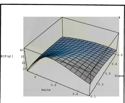
E[P(q)]

gma

0.1

Figure 3.3a

S h o w s the relationship between the optimal delta, the process standard deviation (ranging from 0.1 to 0.5 ) and the m a x i m u m profit.

It is to be expected that an increase in sigma leads to a decrease in profit.

This is shown clearly in Figure 3.3b. The flatness of the optimal profit curve as the

standard deviation of the process gets bigger, should be noted.

Figure 3.3b

Figure 3.4 illustrates the effect of change in the ratio B / A on the optimal

process setting. It should be observed that for small a ( in this case 0.1) the

optimal target setting seems to be approximately constant regardless of changes in

B/A or the standard deviation of the process. Note that the result obtained from

figure 3.2 is also clearly visible in Figure 3.4.

Figure 3.4

Shows 3 pairs of curves. Each pair has assigned the same two values for standard deviation (0.3 and 0.6) but different a values (0.1, 0.3 and 0.5);

A more precise analysis of the relation between the optimal target value of

the process and B/A is shown in Table 3.3, which illustrates the percentage change

in 80 due to change in pricing policy. It can be observed that for relatively small

a, if a increases by 100% then even a large increase in the ratio of B over A has a

minor effect on optimal 8.

a

0.1

0.1

0.3

0.3

0.5

0.5

a

0.3

0.6

0.3

0.6

0.3

0.6

S h o w s the percentage change in optimal process setting due to change in the ratio B to A . T h e distance between L and L 0 varies from 0.1 to 0.5,

T h e further L0 is from L (i.e. the larger the a ) the bigger the effect of B / A on optimal 8. These changes will be larger for smaller o.

Figure 3.5 illustrates the result of relaxing or tightening the distance

between L and L0 on the optimal solution. An increase in a reduces the value of the optimal 8 i.e. brings it closer to L0. This effect is more significant for small values of a as well as bigger ratios of B/A. As a increases, this effect diminishes.

to

s

••a

o

.4

•3'

.2-

.1-O.O

-1,

.1

___f5__-**

^A^^___. *•* ^^^^^^_______.

00 .200 .300 .400 .500 .600 .700 .800 .9

a

o= 0.3

B/A = 0.3

B/A = 0.4

• • • • i

B/A = 0.5

B/A = 0.6

• — H I

B/A = 0.7 00

Figure 3.5

Shows curves of optimal delta values against values of alpha for sigma = 0.3 and B / A from 0.3 to 0.7.

3.3 Concluding remarks

The results would seem to indicate that even if the process variance

CHAPTER 4

Mean Selection

4.1 Introduction

Many types of filling processes exist in practice, that considered here, is with

the intent of obtaining the most appropriate mean setting to maximise profit per item . Overflowed material can either be recaptured or lost; under-filled containers can

either be 'topped-up' and sold for a regular price, or emptied out and material put back into the process or they can simply be discarded. The latter would be typical of the food or pharmaceutical industries where material cannot be re-used, mainly for hygienic reasons. Other authors have addressed a similar problem, however they have assumed containers to have infinite capacity and their cost to be negligible. The issue of whether or not the obtained optimum meets 'Weights and Measures' requirements

has not previously been discussed. In practice, overflow can occur during filling, with or without a loss of material and meeting weight (or volume) specifications is

enforced by law. Overfilling is a real problem in industry, not only due to excess material that is 'given-away' when the containers are overfilled but also in some instances, eg. wine and spirits, where there are penalties for overfilling associated with excise tax. In addition, any container that is hermetically sealed cannot be filled to capacity. In the food industry under-filled containers are invariably discarded. In chemical processes under-filled containers are frequently topped-up or emptied out and the material re-used. Such situations involve different costs and make a

significant difference to the model and its solution.

This chapter explores different types of filling processes and presents

overflow, topping-up the containers or putting the material back into the process. The cost of the containers is also considered as an important part of the model. Model solutions are displayed graphically. The effect of change of the process variance on the optimal solution as well as on the expected profit are both discussed.

In all cases problem solutions are illustrated graphically and results obtained using numerical methods. The latter are obtained on Mathematica. The codes for solution, of each of the models proposed, are shown in the appendix and have proven to be both very easy to use and quick to evaluate.

4.2 General Problem

Consider an automatic filling process where containers are filled with some

ingredient, let this amount be denoted by a random variable X, and without loss of generality assume this to be a measure of volume. It is assumed that X is normally distributed with mean T and known variance a2. A common method of checking that

the process follows a normal distribution is to take a random sample from the process and draw a histogram. Once achieved, control charts can be used to monitor that the process remains in statistical control. The nominal amount of material in each container ( on the label ) is L. According to Weights and Measures Legislation in Australia, containers with a minimum proportion of 0.95 of the stated label content

can be legitimately sold at the regular price. For generality reasons let this quantity be hL, where 0 < h < 1. An automatic device rejects containers with content below hL.

The cost of product in the container is denoted by gx, where g is the cost of material per unit of volume.

T h e aim is to fix the filling m e a n of the process to maximise the expected

profit per container. The Target value, T = hL + 8 ( 8 > 0 ), is called optimal if it maximises the expected profit per container. The inter-relationships between hL, L, L+k and T are shown in Figure 4.1.

Delta

<

Figure 4.1

Inter-relationships between hL, L, L + k and T.

L + k

L

hL

In this chapter a number of variations of the filling process model are

4.3 Theoretical Analysis

The following provides the development of a number of different models for

filling processes together with their analyses. Each solution for the initial setting of the process is displayed graphically, showing a single optimum solution for all

meaningful parameter values. Each solution, as well as the expected profit function, were evaluated using Mathematica.

4.3.1 Finite capacity containers

In these cases overflow is recaptured and reused.

4.3.1.1. Model 1

Consider a filling process where, in the event of under-filling, the product is

reused. This is often the case in the chemical industry for products like dish-washing liquid, washing powder, hair-care products, and paint. In the case of a powder, in order to get the material from inside the box, the boxes have to be cut up and thrown away. In instances of liquids two scenarios are common. If the containers are difficult or very expensive to wash, for example as in the paint industry, the containers are discarded. For containers that are easily washable, like dish-washing liquid or shampoo, the bottles are washed and reused. Two model variations are proposed, for both cases it is assumed that the containers have a capacity of L+k and any overflow is captured at no additional cost.

Model 1-Case 1

The following considers the case where the containers from the under-filled items are

discarded.

Hence if hL<x,

Profit = Selling Price - Filling Cost(including the cost of the container) - Material

Cost.

Thus profit from a single fill attempt may be written as:

P(x) =

S - Cf- Cc- g ( L + k) x > L + k

S - C

f-C

-gx hL<x<L + k

f

x<hL

where S is the selling price and Cf and Cc are the filling cost and the cost of the

container, respectively.

The expected profit per fill attempt, denoted by E[P(x)], is

hL L+k

E[P(x)] = - ( Cf + Cc)Jf(x)dx + J ( S - Cf - Cc -gx)f(x)dx + hL

OO

( S - Cf- Cc- g ( L + k))Jf(x)dx

standardising,

L+k

hL->i L+k-n L+k

E[P(x)] = - ( Cf+ Cc) J(|)(z)dz + ( S - Cf- Cc) J())(z)d2-gjxf(x)dx + hL~H hL

( S - Cf- Cc- g ( L + k)) J(|>(z)dz

L+k-ji

E[P(x)] = - ( Cf+ Cc) < D ^ +

(S-Cf-Cc)

(jL + k-KL-6\ f-8Y!

O

_-o

^ o J J (2)

L+k

g J xf (x)dx + (S - Cf - Cc - g(L + k))

hL

l - O L + k-hL-8^

where ()>(•) and O(-) are the p.d.f. and distribution functions respectively of

the standard normal distribution.

Further simplifications lead to:

E[P(x)] = (S - Cf - Cc - g(L + k)) + g(L + k ) 0

L+k

L + k-hL-S"! (-8}

-SO

VG )

- g ] x f ( x ) d x

hL

where,

L+k-(i

L+k

g j xf (x)dx = g J (oz + p)o())(z)dz =

hL hL-n

go(hL+8)

( fL + k-hL-8"! (S\)

O

_-o

I a J) + gc V v a J

-<$>

f L + k - h L - 8 V

The value of this function for any parameter values can be found by using, for

example, Mathematica (an example is shown in the Appendix). The goal is to find the

target value, T=hL+8, that maximises the expected profit. Hence, one is interested in

the value of 8, say 80, that maximises (2). Numerical methods can be used to find a

solution to (2) and when doing so it is convenient if the first derivative gives only one

optimal solution and the second derivative is always negative thus ensuring that the

obtained optimum is a maxima (i.e. the optimum value of the process setting obtained

from setting the first derivative equal to zero and solving it for 8 by the use of

numerical methods on Mathematica would always return a maxima). A n algorithm to

obtain the optimal mean setting, which can be used for practical purposes, can be

found in the Appendix. To find 80 differentiate equation (2) with respect to 8. Setting

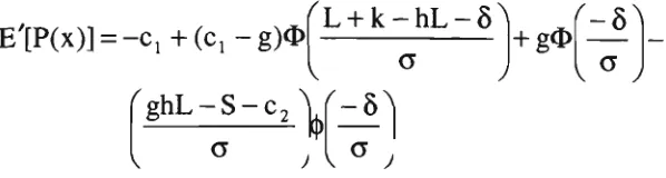
E,[P(x)] = 0, gives:

E'[P(x)] = -(|>

rs^i

y°j

+g

(j-^

_o

K° J

- O

L + k-hL-8Yi

f-^

v ° y

- < | >

v_2__

o

L + k-hL-8^_

r-8^

hL^-S

) \

l

v

(3)

A s shown in the next section, (3) can be used for the graphical illustration of the

solution. Further,

E"[P(x)] = --

f(()

fiP , g,,/L + k - h L - 8 ' £_

lo, o

,

- , / 8 \ ghL8,/8^

/ O l a , a [a,

If E"[P(x)] < 0 (with 8 = 8 0) i.e. if

- o , SghL |

a Sa

ga(()

fL + k-hL-8^1

go

rs

(4)

then 80 is optimal i.e. the solution to (4) will give a setting for the m e a n that will

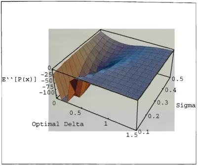
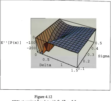
maximise the expected profit. It is shown in Figure 2 that E"[P(x)] is always

Figure 4.2

E"[P(x)] for 0<8<1.5 and 0.1<a<0.5 with L=10,

h=0.95,k=l,S=67,g=3.5.

Model 1-Case 2

The following considers the case where the containers from the under-filled items are

reused. Hence if hL<x,

Profit = Selling Price - Filling Cost - Material Cost.

Thus profit from a single fill attempt may be written as:

P(x) =

S-C

-C

-g(L + k) x > L + k

S-C

-C

-gx h L < x < L + k

-C

- C

otherwise

where S is the selling price and Cf , Cc and Cw are the filling cost, the cost of the

container and the cost of washing the containers from under-filled items, respectively.

The expected profit per fill attempt, denoted by E[P(x)], is

hL L+k

E[P(x)] = -(C

+C

)Jf(x)dx+ J(S-C

-C

-gx)f(x)dx +

( S - C

- C

- g ( L + k))Jf(x)dx

Standardising and putting p = hL + 8 gives,

(D

E[P(x)] = - ( C

+ C J $ A

(S-C

-C

)

(

o

fL + k-hL-SA f-8Yl

_o

L+k

g J xf (x)dx + (S - C

- C

- g(L + k))

^ a J)

l-O

(2)

hL

f L + k - h L - 8 " !

V.

Further simplifications lead to:

E[P(x)] = (S - C

- g(L + k)) + g(L + k)of

J^

1 - (S + C

- C

)0

L+k

- g Jxf(x)dx

hL

where,

L + k-(i L + k

g jxf(x)dx = g J(az+p)a(|>(z)dz =

hL _hL-n

go(hL+8)

(

O

f L + k - h L - 8 " !

;

f-dW

1° JJ

+ga'

f f-^

(H —

-4>

L + k - h L - 8 Y\

E'[P(x)] =

S-C

-C

r-8^1 (J-b

_-4>

V° )

-g

o

a

- O

'L + k-hL-8Y|

o ^ a )

Setting E/[P(x)] = 0, gives the optimal solution.

E"[P(x)] = -

s-c -c Y8^

w

g / L + k-hL-8^1 g/S^i ghL8 f8

+

P\

G {CJ +

-())

vo;

4.3.1.2 M o d e l 2

Consider n o w a filling process where all under-filled containers are

'topped-up'. This is, for example, the case in the production of carbon black. The grade of product used in printer inks, for example, is dispatched in 40kg bags. The filling process involves the product being dispensed from a dual headed filler into the bags which, when filled, pass, by conveyor, to an automatic weighing device where they are automatically rejected if underweight and subsequently topped up by hand. The cost of the bag is far less than the contents and can be considered negligible. The capacity of the container is L+k. Hence, if hL < x < L+ k,

Profit = Selling Price - Filling Cost - Material Cost.

If, however, x<hL the container can be 'topped-up' so that in this instance, Profit = Selling Price - Filling Cost-Additional Processing Cost - Material Cost. Excessive material is assumed captured at no additional cost.

The profit from a single fill attempt m a y be written as:

P(x) =

S - Cf- g ( L + k),

S-C

-gx,

[S-C

-C

-gL,

x > L + k

h L < x < L + k

x< hL

where Ct represents the additional filling cost associated with containers that have to

be 'topped-up'. It is assumed that each under-filled container can be 'topped-up'

exactly to the label specification, L.

Proceeding as previously, the expected profit per fill attempt is:

E[P(x)] = S - Cf- g ( L + k) + g[L(l-h) + k]0

rL-k-hL-8^

(—1

, G J

rL + k-hL-8^

+ [gL(h-l)-C

]0>

-gSO

+ ga

_<H

L+k-hL-5

-<H

+ gSO

— T

- 8

V G ,

V

Figure 4.3

E[P(x)] against 8 and a with S=67, Cf =12, g=3.5, Ct =20,

L=10, k=l, h=0.95.

Differentiation with respect to 8 gives:

rL+k-hL-S^ r-S^l gL(h-l) r-s^ c

r-s^i

E'[Px = -g<D +gO — - ^ U — )

_n _

V

)

) a \ a ) a\aJ

Setting E'[P(x)] = 0, gives:

G KG

J

_g

O

rL + k-hl-8"! (-6}

_{- O}

G J

Ct- g L ( h - l )

A s Figure 4.4 indicates, there is more than one optimum solution (one m a x i m u m and

one minimum). One of these solutions (the minimum) however, as shown in greater

detail in Figure 4.5, is a point of inflection and also it would provide a value for

process setting beyond the capacity of the container. There is thus only one feasible

optimum solution for the process setting.

Figure 4.4