Article
A Novel Anti-Lock Braking System for Electric Vehicles
Chia-Hung Tu, Chun-Liang Lin *, Meng-Yao Yang and En-Ping Chen
Department of Electrical Engineering, National Chung Hsing University, Taichung 402, Taiwan;
alex1983623@hotmail.com (C.-H.T.); cbr1098@hotmail.com (M.-Y.Y.); s8805112000@yahoo.com.tw (E.-P.C.) * Correspondence: chunlin@dragon.nchu.edu.tw; Tel.: +886-4-2285-1549 (ext. 708)
Abstract: Recently, design of electric scooters (ESs) has commonly adopted brushless DC motors (BLDCMs) in place of brushed DC motors. This invention develops a new anti-lock braking system (ABS), based on a slip-ratio estimator, for ES utilizing the braking force generated by the BLDCM when electrical energy releases to the load yielding an analogous effect of ABS control in gas-engine vehicles. Comparing to mechanical ABS, the design possesses the advantages of rapid torque responses due to fast actuating response. The electrical ABS is realized by associating with kinematic and Short-circuit braking. A current controller is used to adjust the braking force, while the sliding mode control strategy is adopted to regulate the slip ratio for best road adhesion while braking. Real-world experiments have been conducted for functional and performance verification.
Keywords: electrical vehicle; anti-lock braking system (ABS); regenerative brake; control
1. Introduction
The common research issues in electric vehicles (EVs) mostly focus on the battery energy management [1]. As it is the major issue to effectively extend endurance of EVs during on-road riding or driving. Less research tasks lay in the issue of safety such as vehicle braking control.
When a vehicle is braking under critical conditions, such as it encountered with wet or slippery road surfaces or mistakes committed by drivers, usually leads to wheel lock making the vehicle out of control. Therefore, preventing wheel locking-up during the emergent braking process is extremely important and anti-lock braking system (ABS) has been becoming a standard equipment in the modern gasoline-powered vehicles. Regarding the ABS with advanced control technologies, there are various design approaches those can be used to improve the performance of ABS, such as sliding mode control [2, 3], fuzzy logic control [4, 5], adaptive control [6], genetic neural control [7], etc. The reason for adopting brushless DC motors (BLDCMs) in EVs lies in its superior characteristics in output power and longer lifespan over brushed DC motors [8, 9]. Parameterized modeling of ESs is the preliminary step while considering the design of ES speed controller [10, 11]. The magic formula tyre model (MFTM) [12] is adopted here which describes the relationship between the slip ratio and wheel friction force. In general, the vehicle speed can be measured from the non-driving wheel or integration of the acceleration sensor. However, the non-driving wheel speed doesn’t exist while the vehicle is decelerating, because the mechanical brakes are set up at each wheel. Integration of the value may diverge because it integrates the offset of the acceleration sensor. To resolve the problem, a slip ratio estimation and control scheme without the need of detecting vehicle speed are proposed in [13, 14]. A non-mechanical antilock braking system (ABS) controller for electric scooters (ESs) based on regenerative, kinetic, and short-circuit braking mechanisms with a boundary layer speed control has been proposed by our research team [15] with two patents received [16, 17].
A new design of ES’s ABS considering the dynamic and short-circuit braking functions is developed in this paper which is closely related to our invention [19] unveiled recently. The kinetic ABS brake makes the BLDCM connect to a high-power low-resistance resistor for energy dissipation in an intermittent manner. This can also be used for a regenerative brake. However, this is not within the scope of this research because the major purpose of it is for battery recharge rather than braking due to the low braking torque. For the short-circuit brake, the BLDCM directly connects to the ground for largest energy dissipation in an intermittent manner with extremely short duty. Sliding mode control is utilized as the strategy for realizing the function of ABS which considers the nonlinear time-varying dynamics of the scooter’s slip ratio. We introduce a new slip ratio estimator without resorting to the vehicle speed measurement, which is unlike those of the traditional ways in the existing gasoline-powered vehicles. A sliding mode controller is proposed to regulate the slip ratio to reach the ideal value for better road adhesion. Simulation study for the ES running on different road surfaces is presented. Extensive experimental verification has also been conducted. The results show effectiveness of the presented design.
2. System Modelling
2.1. Dynamics for Electric Scooter
The rear-wheel electric drive equipped with a BLDCM propels the rear wheel with a fixed transmission ratio. The dynamics of the BLDCM is simply described by:
m
m m m m L
d
J T B T
dt
ω = − ω − (1)
m m e
T = −K i (2)
where Tm is driving torque of the driving motor, ωm is angular speed of the motor, Jm is inertia of the
motor, Bm is damping coefficient, Km is torque coefficient, ie is phase current, and TL denotes torque
due to load.
w
ω Tb
m
T
-1 -0.8 -0.6 -0.4 -0.2 0 0.2 0.4 0.6 0.8 1 -1
-0.8 -0.6 -0.4 -0.2 0 0.2 0.4 0.6 0.8 1
fr
ic
tio
n c
oe
ff
ic
ie
nt
slip ratio dry road
loose grave road ice road
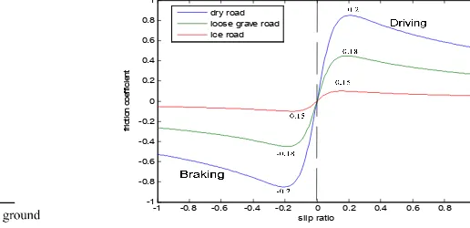
Figure 1. Torque balance on the rear wheel. Figure 2. Friction coefficients vs road surfaces.
Figure 1 shows torque balance on the rear wheel, and the dynamic equation can be described as:
w w w b w w
J ω =T + −T Bω −rF (3)
MV F= (4)
w w
where Jw is inertia of wheel, Tw is driving torque generated, Tb is braking torque, Bw is damping
coefficient of wheel, ωw is angular speed of wheel, r is radius of the rear wheel, F is friction force, M
is total mass of the ES, V is velocity of the ES, and Vw is tangent velocity of the rear wheel. The
transmission system with a fixed transmission ratio can be described by:
,
w n m TL nTw
ω = ω = (6)
where n is the gear ratio. For the experimental platform considered in this research, n=1. Substituting
(1) and (6) into (3), the motion of wheel speed is given as:
2
eq w m b eq w
J ω =nT +nT −B ω −n rF (7)
where Jeq =Jm+n J2 w and
2
eq m w
B =B +n B . In (4), the friction force is the function of friction coefficient u given by:
( )
F=Mgu λ (8)
where g is gravitational constant and
λ
is wheel slip ratio defined by:max( , )
w
w
V V
V V
λ= − (9)
where the denominator of (9) is dependent on the magnitudes of Vw and V . When braking, the wheel
tangent velocity Vw is smaller than the vehicle velocity V , then w
V V V
λ= − .
The tyre model is established based on the Pacejke’s MFTM [12]. The MFTM is formulated upon the experimental results so that the data of braking torque versus the slip ratio are built. Figure 2 shows the friction coefficients versus slip ratio on different road surfaces [20, 21].
2.2. Short-circuit Braking
In the case of a BLDCM with three pairs of stator windings, a pair of switches must be turned on sequentially in the correct order to energize a pair of windings. The back electromotive force (back-EMF) is regarded as the power source, and the current flow is directed from the motor to the dummy load which can be a low-resistance resistor or even short circuit. The power generated by back EMF is E KBL= ωm
where K, B, L are, respectively, motor constant, flux density, and conductor length in motor. Short-circuit brake uses the induced current from the motor back emf to control the input and output current direction of the three-phase voltage by a full-bridge inverter for the purpose of generating a loading effect to the BLDCM; the kinetic brake makes the BLDCM connect to a high-power low-resistance resistor for energy dissipation. This means that the effect of engine brake in gas-powered engines can be mimicked by changing the resistor value of the dummy load. When the lower arm transistors are turned off, the braking current will go through diodes D1 and D4. The electrical energy dissipates in the braking resistor Rb.
The braking resistor using as a dummy load can be a low-resistance resistor or even short circuit, see Figure 3. In Figure 3(b),
( )
a
e e b a
di
E L R R i
dt
= + + (10)
where ia is phase current of the phase a, Re and Le are, respectively, phase resistor and inductance. The
braking power output generated from the EV generator is then P Ei= a. The braking power is accordingly
m a
1 S 2 S 3 S 4 S 5 S 6 S 1 D 2 D 3 D 4 D 5 D 6 D a v b v c v b R C a E R R R
L L L
b
E Ec
a i E e L e R b R
(a) (b)
Figure 3. Short-circuit braking mode (a) current flow low arm transistors when switched OFF (b)
equivalent circuit.
2.3. Slip ratio estimation
Precise velocity of a vehicle during moving is usually difficult to obtain. Here, we extend the slip ratio estimator without measuring vehicle velocity and its acceleration [13].
From (7), the friction force is obtained as
2
m b eq w eq w
nT nT B J
F
n r
ω ω
+ − −
= (11)
Taking differentiation with respect to time of (9) gives Vw VV2w
V V
λ = − . Incorporating (5), (7) and (11) yields
2 2 2
(1 ) ( m b eq w eq w)(1 )
w
w w
nT nT J B
n r M
ω ω ω λ λ λ ω ω + − − = + − + (12)
From the above equalities, it is seen that the unknown variable is only λ . Thus, a slip ratio estimator (SRE) can be designed as
2 2 2
ˆ w(1 ˆ) ( m b eq w eq w)(1 ˆ)
w w
nT nT J B
n r M
ω ω ω λ λ λ ω ω + − − = + − + (13)
where λˆ denotes the estimate of slip ratio. To analyze the convergence of SRE, the estimation error is defined as e= −λ λˆ. The error dynamics is given by
2 2 (2 ˆ)
m b eq w eq w
w
w w
nT nT J B
e e
n r M
ω ω ω λ λ ω ω + − − = − + + (14) Or equivalently 1 ˆ (2 ) w w
e V V e
V λ λ
= − + +
(15)
Clearly, the estimation error e will converge to zero, if
ˆ
(2 )
w
Because λ is very small, the inequality will be closed to Vw<V(2+λˆ)
. Since, when vehicle braking, 0
w
V ≤ , V≤0 and Vw≤V (wheel will be stopped before vehicle), and because λ is very small, thus (16) would be satisfied naturally.
3.Control Design
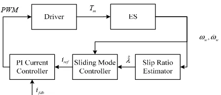
A wheel-slip controller is designed to achieve a target (desired) slip ratio for a given driving condition. The design of ABS utilizes the braking force generated from the BLDCM of the rear wheel when electrical energy releases to the dummy load as the braking action occurs. A PI current controller is designed to determine the duty cycle of pulse width modulation (PWM) at each sampling instant according to the difference of braking and reference currents. In which, a slip-ratio sliding mode controller is proposed to calculate the reference current as the reference input to the PI current controller. Figure 4 shows the control scheme of the overall system.
,
w w ω ω
ref
i
fdb
i
m
T
ˆ
λ
PWM
Figure 4. Overall braking control scheme.
3.1. Control for slip ratio
From (12), control of the ES’s slip ratio is a nonlinear control problem. Sliding mode control provides an effective method to control a nonlinear plant which is one of the simpler approach for the robust control problem [2, 3, 21]. Here, a sliding mode controller is designed to regulate the slip ratio for the best road adhesion. The design procedure of the sliding mode control methodology consists of two steps: first, a sliding surface that models the desired tracking performance is defined; then, a control law such that the state trajectories forced toward the sliding surface is developed. Equation (12) can be rearranged as follows
1( , ) 1( , ) 1
f t b t u
λ= λ + λ (17)
where 1( , ) (1 ) ( 2 2 )(1 ) ,2
eq w eq w
w
w w
J B
f t
n r M
ω ω
ω
λ λ λ
ω ω
+
= + + + 2
1 2
1
( , ) ( )(1 )
w
b t
nr M
λ λ
ω
−
= + and u1=Tm = −K iT.
The sliding surface is chosen as s c=
λ
where c is a constant, λ λ λ= − idl with λidl being the idealvalue of λ. Differentiating s with respect to time gives
s=cλ (18)
By equating (18) to zero, the equivalent control can be obtained as
2
1
eq w eq w w
eq
J B
nr M u
n
ω ω
ω λ
+
= +
+
(19)
To satisfy the sliding condition, the total control law is set to be:
1 eq sgn( )
In real-world applications, the system parameters are mostly uncertain. Considering the major system uncertainty, the control input should be chosen as
1 2 0
0
1
( ( , ))
( , )
u u f t
b λ t λ
= − (21)
where
u
2 is to be determined, 0 2 2 2 0( , ) w(1 ) ( eq w eq w)(1 )
w w
J B
f t
n r M
ω ω
ω
λ λ λ
ω ω
+
= + + + and 0 2 2
0
1
( , ) ( )(1 )
w
b t
nr M
λ λ
ω
−
= +
where M0 =0.5(Mmax+Mmin) is the nominal value of M, Mmin and Mmax denote the lower and upper
bounds respectively. Then, the system can be expressed as
2 d bu
λ= + (22)
where b M M= 0 −1, w(1 ) n w
d ω λ M
ω
= + Δ with n 0
M M M
M
−
Δ = and ΔnM ≤εm.
Suppose that
min max
d < <d d (23)
where min w(1 min) m w
d ω λ ε
ω
= + and max w(1 max) m w
d ω λ ε
ω
= + specify the lower and upper bounds, respectively.
Estimate of d is given by ˆ min max 2
d d
d= + . Then d dˆ− ≤Dwhere D= dmax−dmin . The input gain is
bounded by
min max
0<b ≤ ≤b b (24)
where the geometric mean of bmin and bmax can be defined as the estimate of b as bˆ= b bmin max . From the
above equations, one obtains
1 bbˆ1
ϕ− ≤ − ≤ϕ (25)
where ϕ= b bmax min−1 . The control law u2 in (21) is proposed as follows
(
)
1
2 ˆ ˆ asgn( )
u =b− − −d k s (26)
To satisfy the sliding condition, let us consider
{
}
(
)
1
1 1
1 1
ˆ [ ˆ sgn( )]
ˆ ˆ(1 ˆ ) ˆ
ˆ ˆ 1 ˆ ˆ
a
a
a
ss s d bb d k s
s d d d bb bb k s
s d d d bb bb k
−
− −
− −
= + − −
= − + − −
≤ − + − −
(27)
Set
1 1
ˆ ˆ 1 ˆ ˆ a
d d d bb bb k
where η is a positive constant which determines the convergent rate of λ reaching the sliding surface. Obviously, the following sliding condition will be satisfied
ss≤ −ηs (29)
Since η+ − +d dˆ dˆ 1−bbˆ−1 −bb kˆ−1 a≤ + +η D dˆ ϕ− −1 ϕ−1ka, the gain in (26) becomes
ˆ
( 1)
a
k =ϕ η+ +D d ϕ− (30)
To reduce the chattering effect for reliability in the real-world application, the sign function could be replaced by a saturation function given by
1, if sat( , )= / , if 1, if
s
s t s s
s
ε
ε ε
ε >
≤
− <
(31)
where ε>0 specifies the boundary layer thickness. Chattering can be eliminated for the controller to perform properly in practical applications. The saturation function in (31) is effective to smooth out the control continuity in a thin boundary layer neighboring the switching surface. One is referred to [22] for the similar treatment.
3.2. PI Current Control
The PI current controller is designed to track the reference current computed by the slip ratio sliding mode controller. The input to the PI current controller is
i ref fdb
e
=
i
−
i
(32)where ei is the difference of reference and feedback current, iref is reference input, ifdb is feedback
braking current. The PI current controller with anti-windup before saturation is
( ) ( ) ( )
presat p i
u t =u t +u t (33)
where the proportional term u tp( )=K e tp i( ) and the integral term ( ) ( ) ( ( ) ( )) p
i i c presat
i
K
u t e d K u t u t
T ς ς
=
+ −with upresat( )t being output before saturation,u t( ), output of PID controller; Kp, proportional gain; Ti,
integral time; Kc, integral correction gain. The block diagram of the PI current controller with anti-windup
ref
i
fdb
i
i
e
sat
e
presat
u u
i
u
p
u
max
u
min
u
p
K 1
i
T
dtc
K
Figure 5. Block diagram of the PI current controller with anti-windup correction.
3.3. Operational Procedure
When the driven wheel of ES reaches the predefined speed threshold, the braking procedure works according to the following steps:
Step 1: Acquire Hall sensor’s signals from the BLDC motor. Step 2: Estimate the slip ratio from the slip ratio estimator via (13).
Step 3: Calculate the ideal braking current from the sliding mode controller as the reference input to the PI current controller. The control law of sliding mode strategy is realized by (33).
Step 4: Determine the duty cycle of PWM from the DSP PI current controller according to the difference of feedback braking (from the current sensor) and reference currents. PI control command is generated via DSP’s PWM function.
ˆ
λ
ref I
Figure 8. The experimental ES. Figure 9. Implementation of the braking
control unit.
The software flowchart of the braking process is in Figure 6. In which, braking current is measured constantly. The DSP determines which transistors should be turned on according to the Hall signals which are used to determined rotational speed of the motor. Based on the feedback commands, the DSP calculates the value of duty cycle to adjust the braking force which regulates the slip ratio into the ideal value for best road adhesion.
4.Experimental Verification
4.1. Experimental settings
The experimental ES, block diagram of the designed system, and hardware implementation of related circuits are displayed in Figures 7-9, respectively. The parameters used for simulation of controlling the braking current are listed in Table 1.
(a) (b)
Figure 10. PI current control (a) braking current, (b) changes of duty cycle.
Table 1. Physical parameters for experimental verification.
Item Numerical value
total mass 120 [kg] wheel radius 0.2 [m]
battery 48[V](12V*4) armature inductance 0.0023 [H]
armature resistance 1.1 [
Ω
] motor inertia 0.000568 [kg-m
2] motor torque constant 0.18 [Nm/A
]The ES’s initial speed was set to be 30 km/hr. The PI current controller is designed to track the reference current determined by the slip-ratio sliding mode controller as mentioned in Section 5. The kinetic energy, however, may decrease during the braking process. The duty cycle (i.e. the percentage of time that current flows over the sampling period) for braking current regulation was increased to keep the optimal slip ratio. Figure 10 shows the PI current control command with the reference current 40A for the braking mode.
4.2. Simulation results of slip ratio control
The sliding mode controller is designed to determine the appropriate braking force which regulates the slip ratio to the ideal value. The braking scenes in the short-circuit braking mode are simulated on three different road surfaces: dry road, loose gravel road and iced road. The ideal slip ratio values of three road surfaces are respectively 0.2, 0.18 and 0.15. The bounds of parameters are estimated as follows. Suppose that the mass of the ES with the rider varies within the following range:
min( 150 ) max( 240 )
M = kg ≤M ≤M = kg
The nonlinear time-vary term d varies within the following range
min( 0.1428) max( 0.1142)
d = − ≤ ≤d d =
This gives ˆ min max,ˆ 0.0286
2
d d
d= + d = − . Accordingly, the estimation error of d is bounded by ˆ ( 0.5069)
d d− ≤D = . The upper and lower bounds of the input gain are obtained as
min( 0.75) max( 1.2)
b = ≤ ≤b b = . Thus, the geometric mean of it is bˆ= b bmin max =0.9487 and hence 1( 0.7906) b b1ˆ ( 1.2649)
ϕ− = ≤ − ≤ =ϕ .
Figures 11-13 show, respectively, the simulated results of slip ratio control on dry, loose gravel and ice road surfaces. It’s clearly seen that the slip ratio is controlled to approach the ideal value on ice road surface while braking current is capable of tracking the reference current at the first 2.8sec. Since the wheel speed drops, the back EMF is not enough to support braking current after 2.8 seconds. EV speed decreases accordingly and EV steering can be controlled well. The braking current cannot track the reference current after 3.8 sec and ABS is out of action because of the decrease of kinetic energy. This shows that the present approach works satisfactorily on dry surface and gravel surface but not on ice surface.
0 0.1 0.2 0.3 0.4 0.5 0.6 0.7 0.8 0.9 1
-0.25 -0.2 -0.15 -0.1 -0.05 0
time(sec)
sl
ip
r
ati
o
est silp slip
0 0.1 0.2 0.3 0.4 0.5 0.6 0.7 0.8 0.9 1
0 1 2 3 4 5 6 7 8
9 Wheel and vehicle speed
time(sec)
sp
ee
d(
m
/s
)
wheel speed vehicle speed
0 0.1 0.2 0.3 0.4 0.5 0.6 0.7 0.8 0.9 1
0 50 100 150 200
250 Slip ratio control on dry road surface:
time(sec)
re
fe
re
nc
e c
urre
nt
(A
)
0 0.2 0.4 0.6 0.8 1 1.2 1.4
0 0.1 0.2 0.3 0.4 0.5 0.6 0.7 0.8
0.9 Duty Cycle
time(s)
du
ty
c
yc
le
(a) (b) (c) (d)
Figure 11. Slip ratio control on dry road: (a) slip ratio and estimated slip ratio (b) wheel speed and
0 0.2 0.4 0.6 0.8 1 1.2 1.4 1.6 1.8 -0.25 -0.2 -0.15 -0.1 -0.05 0 time(sec) sl ip r ati o est silp slip
0 0.2 0.4 0.6 0.8 1 1.2 1.4 1.6 1.8
0 1 2 3 4 5 6 7 8
9 Wheel and vehicle speed
time(sec) sp ee d( m /s ) wheel speed vehicle speed
0 0.2 0.4 0.6 0.8 1 1.2 1.4 1.6 1.8
0 20 40 60 80 100
120 Slip ratio control on loose gravel road surface:
time(sec) re fe re nc e c urre nt (A )
0 0.2 0.4 0.6 0.8 1 1.2 1.4
0 0.1 0.2 0.3 0.4 0.5 0.6 0.7 0.8
0.9 Duty Cycle
time(s) du ty cy cl e
(a) (b) (c) (d)
Figure 12. Slip ratio under sliding mode control on the loose gravel road: (a) slip ratio and estimated
slip ratio, (b) wheel and vehicle speed, (c) reference current, (d) PWM duty cycle.
0 2 4 6 8 10 12 14 16
-0.16 -0.14 -0.12 -0.1 -0.08 -0.06 -0.04 -0.02 0 time(sec) slip ra tio est silp slip
0 2 4 6 8 10 12 14 16
0 1 2 3 4 5 6 7 8
9 Wheel and vehicle speed
time(sec) spee d( m /s ) wheel speed vehicle speed
0 2 4 6 8 10 12 14 16
0 5 10 15 20 25 30 35
Slip ratio control on ice road surface:
time(sec) re fe renc e c ur rent ( A ) reference current braking current
0 2 4 6 8 10 12 14 16
0 0.1 0.2 0.3 0.4 0.5 0.6 0.7 0.8 0.9 time(sec) du ty cy cl e
(a) (b) (c) (d)
Figure 13. Slip ratio control on ice road: (a) slip ratio and estimated slip ratio, (b) wheel speed and
vehicle speed, (c) braking current and reference current, (d) PWM duty cycle.
4.3. Experimental results
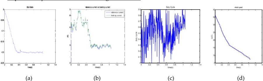
As for the friction coefficient between tire and dry road, the slip ratio becomes the minimum value near to -0.2 as shown in Figure 2, results in the maximum brake torque. The slip ratio is confined to the presetting value of -0.2, as shown in Figure 14(a), the braking current is able to track the reference command by the sliding mode controller, as illustrated in Figure 14(b), the duty cycle for braking current regulation was adjusted to keep the optimal slip ratio, as illustrated in Figure 14(c). Braking current here is proportional to braking torque and the wheel speed is adequately reduced by the sliding mode controller, as illustrated in Figure 14(d).
Please visit the following website for the real-world demonstration of the experiment. https://www.youtube.com/watch?v=OgZiLuDNoP0
0 0.2 0.4 0.6 0.8 1 1.2 1.4
0 0.1 0.2 0.3 0.4 0.5 0.6 0.7 0.8
0.9 Duty Cycle
time(s) du ty cy cl e
0 0.2 0.4 0.6 0.8 1 1.2 1.4
5 10 15 20 25 30 35
40 wheel speed
time(s)
ra
d/
s
(a) (b) (c) (d)
Figure 14. Experimental results of the slip ratio estimation under sliding mode control (a) estimated slip
5.Conclusions
This invention has developed a new idea of ABS for ESs based on a slip-ratio estimator which utilizes braking force generated by the BLDCM when the regenerated energy releases to the virtual load. The mathematical models of ES, BLDCM and slip ratio estimator are built for theoretical analysis of the behavior of braking scene. The model has been verified by simulating the ES moving on different kind of road surfaces characterized by Pacejka’s MFTM. Braking performance of the ES is experimentally validated on an experimental test bench which mimics a variety of road scenes. The electrical ABS works well due to the fast torque response of the BLDCM when the ES moves on the slip road with different road surface adhesion. This shows possibility to realize ABS control for ESs which are functionally analogous to that of the gas-engine vehicles in braking torque control and responsive in anti-block braking actions.
Acknowledgement: This research was sponsored by Ministry of Science and Technology, Taiwan under
the grant MOST 104-2221-E-005-093-MY2.
Author Contributions: All the authors contributed equally to this work. All authors read and approved the
final manuscript.
Conflicts of Interest: The authors declare no conflict of interest.
References