Short-term Deflections of Reinforced Concrete Beams

(1)

Scholarship@Western

Electronic Thesis and Dissertation Repository

7-25-2016 12:00 AM

Short-term Deflections of Reinforced Concrete Beams

Caitlin Mancuso

The University of Western Ontario

Supervisor Dr. F. M. Bartlett

The University of Western Ontario

Graduate Program in Civil and Environmental Engineering

A thesis submitted in partial fulfillment of the requirements for the degree in Master of Engineering Science

Follow this and additional works at: https://ir.lib.uwo.ca/etd

Part of the Civil and Environmental Engineering Commons

Recommended Citation Recommended Citation

Mancuso, Caitlin, "Short-term Deflections of Reinforced Concrete Beams" (2016). Electronic Thesis and Dissertation Repository. 3862.

https://ir.lib.uwo.ca/etd/3862

This Dissertation/Thesis is brought to you for free and open access by Scholarship@Western. It has been accepted for inclusion in Electronic Thesis and Dissertation Repository by an authorized administrator of

(2)

ii

ABSTRACT

Excessive deflection of concrete beams is a recurring serviceability problem. Provisions in current building codes, CSA A23.3-14 and ACI 318-14, account for some but not all of the contributing factors. The effect of loading concrete members at very young ages on the associated deflections remains uncertain.

Concrete strain data reported by others are used to investigate if conventional stress-strain relationships, and empirical equations in A23.3-14 for tensile strength and elastic modulus are accurate for young concretes. Moment-curvature analyses based on conventional simplifying approximations used for flexural analysis are performed. For concretes less than one day old, the conventional relationships and empirical equations yield unconservative results. For older concretes, however, the conventional stress-strain relationships, empirical equations and conventional simplifying assumptions yield accurate results.

Current practice is to compute deflections using either a whole-member analysis with an average effective moment of inertia, or a discretized analysis with unique effective moments of inertia for each discrete element. Branson proposed equations for the effective moment of inertia for use in either analysis. Bischoff proposed an improved equation, for use in whole-member analysis only. The current research quantifies suitable modifications to the Bischoff Equation for use in discretized analysis: the exponent applied to the cracking-to-applied moment ratio term should be increased from 2 to 3.

(3)

iii

accurate computation of deflections. The Bischoff Equation with the cracking moment computed using full modulus of rupture yields the best results. When the recommended reduced modulus is used, the difference between results using the Branson and Bischoff Equations is indistinguishable.

(4)

iv

ACKNOWLEDGMENTS

I would like to express my deepest gratitude to my supervisor, Dr. F. M. Bartlett. He has been a wonderful mentor and completing this thesis would not have been possible without his guidance and support. Dr. Bartlett’s passion and dedication to the field of engineering is inspiring, and if I am able to emulate a fraction of that I know I will have a fulfilling career.

Thank you to all the faculty and staff at Western University for making my undergraduate and graduate studies a truly great experience. I am grateful for all of the friendships I have made throughout this journey.

The financial support provided from the Natural Sciences and Engineering Research Council (NSERC), in the form of a Canada Graduate Scholarship (CGS-M), from the Province of Ontario and the Faculty of Engineering at Western University, in the form of a the Queen Elizabeth II Graduate Scholarship in Science and Technology (QEII-GSST) is gratefully acknowledged.

Informal contributions, interest and suggestions from Kevin MacLean, Dr. Tibor Kokai and their colleagues from the Toronto office of Read Jones Christoffersen are also gratefully acknowledged.

(5)

v

LIST OF FIGURES

Figure 2-1: Todeschini (1964) and Modified Hognestad (1951) Stress-Strain Relationships 13!

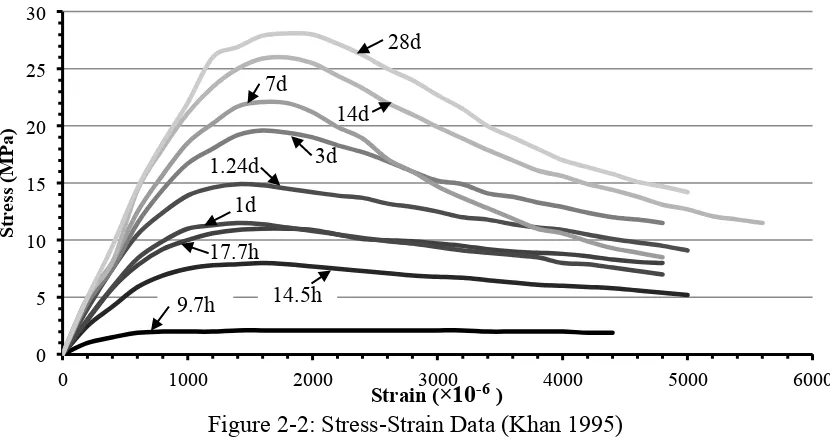
Figure 2-2: Stress-Strain Data (Khan 1995) ... 15!

Figure 2-3: Stress-Strain Data (Jin et al. 2005) ... 16!

Figure 2-4: Stress-Strain Curves, Khan 9.7h ... 17!

Figure 2-5: Stress-Strain from Data, Todeschini & Modified Hognestad Relationships, Khan ... 18!

Figure 2-6: Normalized Stress-Strain Curves from Data, Todeschini & Modified Hognestad Relationships, Khan 9.7h & 1d ... 19!

Figure 2-7: Comparison of Observed and Computed Normalized Elastic Moduli ... 22!

Figure 2-8: Proportionality Constant at Various Ages ... 23!

Figure 2-9: Moment-Curvature Analysis Flowchart ... 25!

Figure 2-10: Trilinear Moment-Curvature Relationship Derived Using Conventional Simplifying Approximations ... 26!

Figure 2-11: Conventional Simplifying Approximations ... 28!

Figure 2-12: Moment-Curvature for Various Stress-Strain Relationships, ρ=0.5% ... 29!

Figure 2-13: Force Equilibrium ... 31!

Figure 2-14: Trilinear Moment-Curvature Relationship, Jin et al. 18h ... 33!

Figure 2-15: Effect of Reinforcement Ratio, Khan ... 34!

Figure 2-16: Flexural Rigidity Based Moment-Curvature Relationships, Khan ... 36!

Figure 3-1: Variation of Ie/Ig with Reinforcement Ratio (after CAC 2016) ... 43!

Figure 3-2: Member Idealizations for Deflection Calculation ... 44!

Figure 3-3: Mesh Sizes ... 48!

Figure 3-4: Analysis of Discretized Three-Span Beam with Different Meshes, Branson ... 52!

Figure 3-5: Analysis of Discretized Simply Supported Beam, Bischoff ... 58!

Figure 3-6: Analysis of Discretized Two-Span Continuous Beam, Bischoff ... 64!

Figure 3-7: Pattern Loading and CAC (2016) Moment Coefficients ... 67!

Figure 3-8: Analysis of Discretized Three-Span Continuous Beam, Bischoff ... 68!

Figure 3-9: Analysis of Discretized Three-Span Continuous Beam, Bischoff, ρ-=0.5% ... 75!

Figure 3-10: Analysis of Discretized Three-Span Continuous Beam, Bischoff, ρ-=1.5% ... 77!

Figure 4-1: Beam N3#10ST – El-Nemr (2013) ... 91!

Figure 4-2: Simply Supported Beams SB-1 (left) & SB-3 (right) – Branson (1965) ... 92!

Figure 4-3: Beam 3-G-Dry – Washa (1947) ... 96!

Figure 4-4: Simply Supported Beam C1 – Corley & Sozen (1966) ... 100!

Figure 4-5: Simply Supported Beam E-1 – Yu (1960) ... 102!

Figure 4-6: Test-to-Predicted Ratios for Various Reinforcement Ratios – Simply Supported Members ... 105!

Figure 4-7: Sensitivity of Test-to-Predicted Ratios to κ ... 111!

Figure 4-8: Two-Span Beam X3,X6 – Washa & Fluck (1956) ... 113!

Figure 4-9: Normalized Effective and Cracked Moments of Inertia - Beam X3,X6 (Washa & Fluck 1956) ... 115!

(8)

viii

(9)

ix

LIST OF TABLES

Table 1-1: Alternative Deflection Calculation Procedures ... 4!

Table 2-1: Todeschini and Modified Hognestad Stress-Strain Relationships ... 12!

Table 2-2: Comparison of Elastic Secant Moduli with Khan (1995) ... 20!

Table 2-3: Comparison of Elastic Secant Moduli with Jin et al. (2005) ... 20!

Table 2-4: Nominal Ultimate Moment and Curvature ... 32!

Table 2-5: Flexural Rigidity Comparison ... 36!

Table 2-6: Effect of ρ on EcIcr ... 37!

Table 3-1: Equations for Weighted Average Iefor Continuous Spans (CSA 2014) ... 44!

Table 3-2: Member Idealization & Equations for Ie ... 45!

Table 3-3: Sensitivity of Maximum Deflection to Mesh Size ... 49!

Table 3-4: Summary of Simply Supported Beam Computed Deflections ... 60!

Table 3-5: Two-Span Continuous Beam Section Properties ... 62!

Table 3-6: Summary of Two-Span Continuous Beam Computed Deflections ... 65!

Table 3-7: Three-Span Continuous Beam Section Properties ... 67!

Table 3-8: Summary of Three-Span Continuous Beam Computed Deflections ... 69!

Table 3-9: Section Properties of Two-Span Continuous Beams with ASTM A1035/A1035M Grade 100 (690) Steel ... 71!

Table 3-10: Section Properties of Three-Span Continuous Beams with ASTM A1035/A1035M Grade 100 (690) Steel ... 71!

Table 3-11: Summary of Computed Deflections of Simply Supported Beams with ASTM A1035/A1035M Grade 100 (690) Steel ... 72!

Table 3-12: Summary of Computed Deflections of Two-Span Continuous Beams with ASTM A1035/A1035M Grade 100 (690) Steel ... 72!

Table 3-13: Summary of Computed Deflections of Three-Span Continuous Beams with ASTM A1035/A1035M Grade 100 (690) Steel ... 73!

Table 4-1: Summary of Simply Supported Studies ... 83!

Table 4-2: Results of UNICIV Report No. R-434 (Gilbert & Nejadi 2004a) ... 86!

Table 4-3: Results of UNICIV Report No. R-435 (Gilbert & Nejadi 2004b) ... 88!

Table 4-4: Results of Washa & Fluck (1952) ... 89!

Table 4-5: Results of El-Nemr (2013) – Specimen N3#10ST ... 90!

Table 4-6: Results of Branson (1965) ... 93!

Table 4-7: Compression Tests of Control Cylinders in study by Washa (1947) ... 94!

Table 4-8: Results of Washa (1947) ... 98!

Table 4-9: Results of Corley & Sozen (1966) ... 100!

Table 4-10: Specimen parameters varied in study by Yu (1960) ... 101!

Table 4-11: Results of Yu (1960) ... 102!

Table 4-12: Overall Findings for Simply Supported Members ... 106!

Table 4-13: Overall Findings for Simply Supported Members – Excluding Studies ... 107!

Table 4-14: Summary of Continuous Beam Studies ... 108!

Table 4-15: Test-to-Predicted Ratios ... 110!

Table 4-16: Two-Span Continuous Beam Section Properties – Washa & Fluck (1956) ... 112!

(10)

x

Table 4-18: Results of Branson’s Two-Span Beams (1965) ... 118!

Table 4-19: Summary of FRP Studies ... 119!

Table 4-20: Results of Two-Span Steel Control Specimens ... 120!

Table 4-21: T-Beam Section Properties – Guralnick & Winter (1957, 1958) ... 123!

Table 4-22: Results Guralnick & Winter (1957, 1958) – T-Beam Members ... 125!

Table 4-23: Overall Findings For Continuous Members ... 128!

Table 4-24: Overall Findings for All Members ... 129!

Table 4-25: Accuracy of Deflection Calculation Procedures – Simply Supported Members ... 132!

Table 4-26: Accuracy of Deflection Calculation Procedures – Continuous Members ... 133!

(11)

xi

LIST OF APPENDICES

Appendix A: Steps for Moment-Curvature Analysis ... 149

Figure A-1: Stress-Strain Curve from Khan (1995) at 1 day ... 150!

Figure A-2: Discretization of Compression Region for Moment-Curvature Analysis .. 150!

Figure A-3: Todeschini Model Moment-Curvature Analysis ... 154!

Figure A-4: Modified Hognestad Model Moment-Curvature Analysis ... 156!

Appendix B: MS Excel Spreadsheet Check Using Ie=Ig ... 160

Table B-1: Comparison of Computed Deflections for Ie=Ig ... 160!

Appendix C: Mesh Sensitivity Analysis with Point Load ... 161

Figure C-1:Pattern Point Loading and CAC (2016) Moment Coefficients ... 161!

Figure C-2: Analysis of Discretized Three-Span Continuous Beam with Different Meshes with a Concentrated Point Load, Branson ... 163!

Table C-1: Sensitivity of Maximum Deflection to Mesh Size – Concentrated Point Load ... 162!

Appendix D: Simply Supported Member Mesh Sensitivity Analysis ... 164

Table D-1: Sensitivity of Maximum Deflection to Mesh Size – Simply Supported Member ... 164!

Appendix E: Determination of m for use with The Bischoff Equation in a Discretized-Element Idealization using SOLVER Function ... 165!

Table E-1: SOLVER values for m in discretized-element idealization ... 165!

Table E-2: Summary of Simply Supported Beam Computed Deflections with m=2 .... 166!

Table E-3: Summary of Two-Span Continuous Beam Computed Deflections with m=2 ... 167!

Table E-4: Summary of Three-Span Continuous Beam Computed Deflections m=2 ... 168!

Appendix F: Other Studies Considered for Verification of Deflection Calculation Procedures ... 169!

Figure F-1: Simply Supported Beam 1B2 – Bakoss et al. (1982) ... 171!

Figure F-2: Two-Span Beam 2B1/2B2 – Bakoss et al. (1982) ... 173!

Figure F-3: Two-Span Beam 1-1 – Mattock (1959) ... 175!

Table F-1: Results of Park et al. (2012) ... 170!

Table F-2: Results of Bakoss et al. (1982) – Simply Supported ... 172!

Table F-3: Results of Bakoss et al. (1982) – Two-Span ... 174!

Table F-4: Results of Mattock (1959) ... 176!

Appendix G: Sensitivity of Test-to-Predicted Ratios to the Value of κ ... 177!

Table G-1: Test-to-Predicted Ratios – Bischoff Equation, Full fr ... 177!

Table G-2: Test-to-Predicted Ratios – Bischoff Equation, 0.67fr ... 178!

(12)

xii

NOMENCLATURE

A% the probability that the actual deflection will be within a range of the predicted value

As area of tensile flexural reinforcement b width of concrete compression zone bfl flange width of a T-beam

bw web width of a T-beam

c distance from extreme compression fibre to neutral axis c/d maximum neutral axis depth limit for flexural members Cc compressive force magnitude

d distance from extreme compression fibre to centroid of tension reinforcement Ec elastic modulus of concrete

EcIcr flexural rigidity of concrete Es elastic modulus of steel

f0 compressive strength of concrete

f’c specified compressive strength of concrete fc concrete compressive stress at extreme fibre fct split cylinder strength (mean value = f_ct)

fr modulus of rupture of concrete (mean value = f_r) fy specified yield strength of steel

h overall thickness or height of member

Icr moment of inertia of cracked section transformed to concrete Ie effective moment of inertia

Ig moment of inertia of gross section

k1 ratio of the average concrete compressive stress to the maximum stress

k2 ratio of the distance between the extreme compression fibre and the resultant of the compressive force to the depth of the neutral axis

k3 ratio of the distance between the extreme compression fibre and the resultant compressive force for the trapezoidal portion of the Modified Hognestad stress-strain curve to the depth of the neutral axis

kd depth from the extreme compression fibre to the neutral axis, elastic-cracked analysis

L span length

m exponent applied to the Mcr/Ma term in effective moment of inertia equation M0 nominal applied bending moment

Ma applied bending moment (in positive moment region, M+, in negative moment region, M-)

Mcr cracking moment

Mf moment due to factored loads

Mf6 ultimate flexural resisting moment, according to the Appendix of ACI 318-56 Mn nominal moment capacity

Mr factored flexural resistance Ms moment due to service loads My yield moment

(13)

xiii P concentrated point load

PL probability that a test-to-predicted ratio will fall below a range PU probability that a test-to-predicted ratio will fall above a range s sample standard deviation

Ts tensile force magnitude

w applied uniformly distributed load

wf factored applied uniformly distributed load wL/wD live-to-dead load ratio

yt distance from centroidal axis of section to the extreme fibre in tension x the ratio of the extreme compression fibre strain to the strain at peak stress

x sample mean

Z unit value of the standard normal distribution Greek Symbols

γc density of concrete

∆mid midspan deflection of a member ε concrete compressive strain

ε0 concrete compressive strain at peak stress εs tensile strain in flexural reinforcement

εult ultimate extreme fibre concrete compression strain εy yield strain of steel

κ weighting coefficient

ρ flexural reinforcement ratio (in positive moment region, ρ+, in negative moment region, ρ-₎

σc concrete compressive stress σs steel tensile stress

Ψ curvature of a flexural member

(14)

CHAPTER 1:

INTRODUCTION

1.1 BACKGROUND

Excessive deflection of concrete floor slabs is a recurring serviceability problem (Gilbert 2012, Stivaros 2012). Others have investigated contributing factors including: construction methods and associated loading (Kaminetzky & Stivaros 1994), cracking due to restrained shrinkage, creep and flexure (Bischoff 2007, Scanlon & Bischoff 2008), and early-age concrete properties (ACI 435 1995, Khan 1995). Provisions in current building codes, CSA A23.3-14 in Canada (CSA 2014) and ACI 318-14 in the United States (ACI 2014), account for some but not all of these effects. The effect of loading concrete members at very young ages (3 days is not uncommon given current construction practices) on the associated deflections remains unknown. Construction loads may subject young concrete to large bending moments causing flexural cracking. Accurate predictions of the modulus of rupture, the elastic modulus and the cracked moment of inertia, are necessary because computed deflections are sensitive to these properties.

Conventional Material Property Quantification for Concrete 1.1.1

(15)

concretes (MacGregor & Bartlett 2000). There is a need, therefore, to quantify the difference in compressive stress-strain response and verify that conventional idealizations and simplifications conventionally assumed for flexural analysis can accurately predict the flexural behaviour of young-age concrete.

Common practice is to use stress-strain idealizations derived from mature concrete, i.e., the Todeschini and Modified Hognestad relationships, to determine the compressive response of concrete in compression. It is unclear however if the simplifying approximations conventionally adopted in flexure theory, such as the compressive stress block idealization at the ultimate limit state, are valid for young concretes.

The ascending portion of the moment-curvature response is of particular interest for deflection calculations, and is often approximated by the cracked flexural rigidity, EcIcr, of the member. It is therefore necessary to predict accurately the elastic modulus, Ec, and cracked moment of inertia, Icr, and so determine if this conventional simplifying approximation still holds for young concretes.

Effective Moment of Inertia for Computation of Instantaneous Deflections 1.1.2

(16)

inertia. The two most familiar equations for calculating the effective moment of inertia were developed by Branson (1965) and Bischoff (2005). Current practice is to compute deflections idealizing the member as either a single element, where an average effective moment of inertia is assigned to the entire member, or a number of discrete elements, where the member is idealized as discrete elements, each with unique effective moments of inertia.

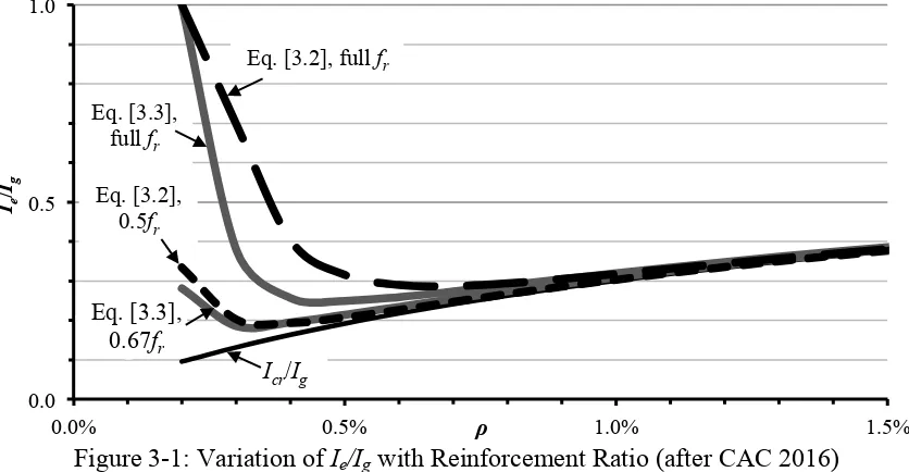
Branson originally proposed two equations for effective moment of inertia, a 3rd-power equation for use in single-element idealization and a 4th-power equation for use in discretized-element idealization. These two equations are based, however, on an incorrect mechanical model that idealizes the stiffnesses of the cracked and uncracked regions as springs in parallel, when they should be in series (Bischoff 2007). Therefore, Branson’s method overestimates the tension stiffening effect and is unconservative, especially for lightly reinforced members (CAC 2016). Bischoff has proposed a single equation, based on the correct mechanical model, for use in the single-element idealization only. It is necessary to determine a modification to allow use of the Bischoff Equation to compute the deflection of a discretized member.

(17)

With any method of analysis, the accuracy of the deflection calculation depends upon the accuracy of the analysis including the quantification of the input parameters (ACI 435 1995). It is impossible to eliminate inaccuracy caused by the uncertainty of the input parameters because the interaction between factors affecting concrete deflections is highly complex. The accuracy of the analysis can however be quantified, and it is necessary to do so for the various alternative deflection calculation procedures.

Flexural members are subjected to tensile stresses due primarily to restraint of concrete shrinkage. When using the Branson Equation, A23.3-14 (CSA 2014) requires that the cracking moment, Mcr, be calculated using a reduced modulus of rupture, 0.5fr, for beams, one-way and two-way slabs. When using the Bischoff Equation, Scanlon and Bischoff (2008) recommend that Mcr be calculated using 0.67fr. Therefore, these recommended modulus of rupture reductions must be considered when quantifying the various procedures. There are therefore eight alternative deflection calculation procedures, shown in Table 1-1, involving: the Branson or Bischoff Equations, the single-element or discretized-element idealizations, and the full or reduced moduli of rupture.

Table 1-1: Alternative Deflection Calculation Procedures

Equation Branson Bischoff

Idealization Single-Element m =3

Discretized-Element m =4

Single-Element m =2

Discretized-Element m =?

Modulus of Rupture

Not Considering Restraint of Shrinkage Full fr

Considering Restraint of Shrinkage 0.5fr

(18)

1.2 OBJECTIVES

The primary objective of the research reported in this thesis is to provide guidance for the accurate computation of deflections, including identification of the key influencing factors and recommendations concerning young-age concrete. The specific objectives of this research are as follows:

1. To determine if conventional stress-strain idealizations and empirical equations to quantify material properties can reasonably model stress-strain data and material properties determined experimentally for young concretes (e.g., Khan 1995, Jin et al. 2005).

2. To verify the accuracy of the Branson 4th-power equation and to determine a similar modification to the Bischoff Equation for use in a discretized analysis. 3. To quantify the accuracies of deflections computed using the various alternative

deflection calculation procedures using experimentally observed values and to also identify factors necessary to compute deflections accurately.

1.3 OUTLINE OF THESIS

(19)

analyses based on conventional simplifying approximations, the reported concrete stress-strain data, and the Todeschini and Modified Hognestad relationships are performed to quantify the accuracy of these methods for young-age concretes.

Chapter 3 presents the Branson and Bischoff Equations for the effective moment of inertia and typical single-element and discretized-element idealizations for deflection calculations. Test cases of flexural members with various end fixities, reinforcement ratios, and live-to-dead load ratios are explored to quantify suitable modifications to the Bischoff Equation for use in discretized-element idealizations. A mesh sensitivity analysis is performed to determine the largest practical mesh size for design office use.

Chapter 4 presents an investigation of the accuracy of the various alternative deflection calculation procedures by comparing predicted deflections to observed values for simply supported and continuous test beams reported by others. Deflections are computed based on the material properties, section geometry and other relevant data reported and test-to-predicted ratios are calculated. Factors that have a major impact the accuracy of computed deflections are also investigated. The database of members investigated covers a wide range of reinforcement ratios, span-to-depth ratios, and section geometries, subjected to varying curing conditions and applied loadings.

(20)

CHAPTER 2: EARLY-AGE CONCRETE

2.1 IMPORTANCE OF EARLY-AGE MATERIAL PROPERTIES FOR DEFLECTIONS

The commentary to ACI 318-14 (2014) cautions, “At early ages, a structure may be adequate to support the applied loads but may deflect sufficiently to cause permanent damage.” Concrete strength and stiffness properties are important for deflection calculations and at very young ages are influenced by the following factors related to construction (Kaminetzky & Stivaros 1994):

• The chosen construction techniques – curing and finishing methods impact the concrete material properties at a given age.

• The general construction schedule – accelerated construction schedules mean that concrete slabs may not have reached appreciable strength when significant construction loads are applied (ACI Committee 347 2005).

Large bending moments applied to young concrete cause flexural cracking. Accurate prediction of the modulus of rupture at young ages is, therefore, important for flexural members. Deflection calculations are particularly sensitive to the computed member stiffness, so it is also necessary to quantify accurately the elastic modulus, Ec, and the cracked moment of inertia, Icr.

(21)

such specification. ACI Committee 347 (2005) provides slightly more guidance and recommends formwork be designed for a minimum design value for combined dead and live loads of 100lb/ft2 (4.8kPa).

Construction loads may be beyond the control of the designer, but the removal of formwork for multistory construction should be a part of a planned procedure considering the concrete strength and age at transfer (ACI 2014). Typical floor construction cycles, i.e., from the casting of a concrete slab to the removal of shores and casting of the subsequent slab above, range from 3.5 to 7 days (Monette & Garnder 2015). A prudent contractor would likely not remove the formwork if the concrete is less than 3 days old. Grundy and Kabaila (1963) have demonstrated that, using conventional shoring systems, a slab can experience construction loading as great as 2.25 times its self-weight at 14 days after casting.

Characteristics of Early-Age Concrete 2.1.1

(22)

Concrete strength and other material properties, such as the elastic modulus, Ec, and the modulus of rupture, fr, increase with age. Two empirical relationships are given in CSA A23.3-14 (CSA 2014) to quantify the secant modulus, that corresponds to the slope of the line drawn from a stress of zero to a compressive stress of 0.40f’c. For concretes with a density, γc, between 1500 and 2500 kg/m3 the equation for Ec is:

[2.1] E_c=(3300 f'_c+6900) ₂₃₀₀γc 1.5

Alternatively, for normal density concretes with compressive strengths from 20MPa to 40MPa:

[2.2] Ec=4500 f'_c

It is implied in A23.3 that the empirical relationship for Ec given in Eq. [2.1] is preferred. For normal density concretes, however, Eq. [2.2] predicts more conservative Ec values at low compressive strengths and is therefore used in the analysis of very young concretes.

The CSA A23.3-14 (CSA 2014) equation for the modulus of rupture, fr, is:

[2.3] f_r=0.6 f'_c

The modulus of rupture is proportional to the square root of the compressive strength and the proportionality constant of 0.6 is intended to represent a lower bound of the experimental data (CSA 2014).

(23)

relationships have been commonly used to idealize the stress-strain relationship for normal strength concrete in compression and have longstanding credibility in this role (MacGregor & Bartlett 2000). The flexural behaviour of sections at young ages can therefore be quantified given variations of the concrete stress-strain relationship. This also facilitates verification of various common simplifications of the flexure theory, such as the compressive stress block idealization in CSA A23.3-14 (2014), at young ages.

Deflections depend on member stiffness and so on the flexural rigidity, EcIcr. Therefore, to compute accurate deflections, both the elastic modulus and cracked moment of inertia must be accurate. For a rectangular cross section without compression reinforcement, the cracked moment of inertia, Icr, is given (e.g., MacGregor & Bartlett 2000) by:

[2.4] I_cr=b kd3

3 +nAs(d-kd) 2

where b is the section width, d is the depth to the reinforcement, n is the modular ratio, Es/Ec, As is the area of steel and kd is the depth to the neutral axis. The factor k, used to locate the neutral axis depth, is computed as:

[2.5] k= 2ρn+ ρn 2₋_ρn

Chapter Objectives 2.1.2

(24)

1. To determine the age at which the experimental stress-strain data (e.g., Khan 1995, Jin et al. 2005) can be reasonably modeled using the Todeschini (1964) and the Modified Hognestad (1951) compressive stress-strain relationships.

2. To determine if experimentally determined material properties (e.g., Khan 1995, Jin et al. 2005) can be reasonably modeled using the CSA A23.3-14 empirical relationships for the elastic modulus, Eq. [2.2], and modulus of rupture, Eq. [2.3].

3. To determine if the moment-curvature response derived from experimental stress-strain data (e.g., Khan 1995, Jin et al. 2005) can be reasonably modeled using typical simplified idealizations commonly adopted in the theory of flexure for reinforced concrete (e.g., MacGregor & Bartlett 2000).

4. To quantify any differences in the flexural rigidity, EcIcr, for varying material properties, concrete ages, and reinforcement ratios, as computed using the A23.3 (CSA 2014) empirical equation for the elastic modulus of concrete, Eq. [2.2], or using secant moduli computed from experimental data for young age concretes.

2.2 STRESS-STRAIN CURVES FOR EARLY-AGE CONCRETE

(25)

Todeschini and Modified Hognestad Stress-Strain Relationships

2.2.1

The Todeschini relationship provides a convenient idealization of concrete in compression. As shown in Table 2-1 and Figure 2-1, the entire stress-strain curve is given by one continuous function. It provides convenient closed-form solutions for the magnitude and location of the resultant concrete force at a given extreme fibre strain. The concrete stress, fc, is a function of the 28-day specified concrete compressive strength, f’c, for a given compressive strain, ε, Eq. [2.6]. The strain at peak stress, ε0, is also a function of f’c, and the elastic modulus, Ec, Eq. [2.7]. The ultimate extreme fibre strain, εult, is limited to 0.0035 as prescribed in A23.3-14 (CSA 2014). For the analysis of young concretes, f’c was taken as the maximum concrete stress, f0, at a given age from the experimental data, and the elastic modulus was determined using Eq. [2.2].

Table 2-1: Todeschini and Modified Hognestad Stress-Strain Relationships Relationship Concrete Stress,

fc (MPa) Eq.

Strain at Peak Stress, ε0 Eq.

Ultimate Strain, εult Todeschini

(1964) [2.6] ε0= 1.71f’c/Ec [2.7] 0.0035εult=

Modified Hognestad

(1951)

[2.8] ε0= 1.8f’c/Ec [2.9] _0.0038εult= f_c=2f'c(ε ε0)

1+(ε ε0) 2

f_c= f'_c 2εc ε0

− εc ε0 " # $ % & ' 2 ( ) * * + ,

-- for fc< f'c

fc= f'c 1−.15

εc−ε0

εult−ε0 " # $ % & ' ( ) * + ,

(26)

Figure 2-1: Todeschini (1964) and Modified Hognestad (1951) Stress-Strain Relationships

The Modified Hognestad stress-strain relationship, also shown in Table 2-1 and Figure

2-1, consists of a parabola to a maximum stress at a strain, ε0, computed using Eq. [2.9],

that is 5.2% larger than the ε0 value assumed in the Todeschini relationship, Eq. [2.7].

The descending branch is linear to 85% of the maximum stress at an ultimate strain of

0.0038. When using the Modified Hognestad stress-strain relationship for young

concretes the 28-day specified concrete strength, f’c, was taken as the maximum concrete

stress, f0, at a given age from the experimental data.

Others have investigated empirically the stress-strain response of concrete at early ages.

The experimental data obtained as part of the studies by others was used for analysis, and

was not experimentally obtained as part of this investigation. Khan (1995) performed

modulus of rupture tests and investigated the compressive stress-strain responses of 30,

70 and 100MPa strength concretes at ages from 72 hours to 91 days, and a total of

approximately 300 cylinders were tested in compression. The study also investigated the 0

5 10 15 20 25

0 500 1000 1500 2000 2500 3000 3500 4000

S

tr

es

s (M

P

a)

Strain (×10-6₎

Modified Hognestad Todeschini

ε₀, Eq.[2.9]

(27)

influence of temperature-matched, sealed, and air-dried curing conditions on the initial

temperature rise after casting. For the purposes of the present study, the sealed specimens

with a 28-day concrete strength of 30MPa were investigated because this strength is

typical for concrete floor slabs and the sealing procedure will limit significant shrinkage

effects.

Concrete cylinders, 100×200mm, and flexural beams were cast in plastic moulds that

enabled demoulding at very early ages without disturbing the concrete. The cylinders

were end-capped with a sulphur-based capping compound prior to testing. Compressive

strength and modulus of rupture tests were carried out at 9.7, 14.5 and 17.7 hours, and at

least three cylinders were tested at each of 1, 1.24, 3, 7, 14, 28, and 91 days. To

determine the compressive strengths at very early ages (i.e., less than 24 hours), more

sensitive load cells were used.

Figure 2-2 shows the observed compressive stress-strain responses at various ages. From

an age of one day and beyond, the stress-strain response conforms generally to the

Todeschini or Modified Hognestad relationships: initially linear with reduced modulus to

the maximum stress followed by strain softening. At an age of 9.7 hours, however, there

is no strain softening, so neither the maximum stress nor the corresponding strain at

(28)

Figure 2-2: Stress-Strain Data (Khan 1995)

Jin, Shen and Li (2005) investigated the behaviour of high- and normal-strength concretes at ages between 12 hours and 28 days. The study included compression and splitting tension tests. The cylinder specimens, 100×200mm, were covered with a wet cloth until demoulding, at which point the specimen was either tested or transferred to a climate-controlled curing room. Splitting tension tests were performed on three cylinder specimens at each age. Figure 2-3 shows the complete stress-strain responses that were obtained at ages of 18 hours, 1, 2, 3, 7 and 28 days. To eliminate the influence of any heterogeneous behaviour of the cement gel on the linearity of the stress–strain curve, four loading-unloading cycles at 40% of desired maximum load were applied to the test specimen before the actual test. The complete stress–strain curve was measured after the pre-loading cycle. The compressive stress-strain curve at three days is again generally consistent with the Todeschini and Modified Hognestad relationships. While the sample sizes are relatively small, the data can be used with confidence because both studies were

0 5 10 15 20 25 30

0 1000 2000 3000 4000 5000 6000

S

tr

es

s (M

P

a)

Strain (×10-6₎ 28d

9.7h

14d

14.5h 1d 17.7h

1.24d 3d

(29)

independently performed a decade apart and show similar trends. Both studies indicate that very young concrete does not strain soften, and does not show a clear maximum stress or corresponding strain at maximum stress. Strain softening was observed the young age of three days in both studies.

Figure 2-3: Stress-Strain Data (Jin et al. 2005)

Early-Age Stress Strain Curves 2.2.2

The experimental stress-strain response from Khan (1995) at 9.7 hours is shown in Figure 2-4(a) and (b) with the Todeschini and Modified Hognestad stress-strain curves for the experimentally observed maximum stress, 2.1MPa, and the corresponding strain at peak stress computed using Eq. [2.7] or Eq. [2.9], respectively. Both the Todeschini and Modified Hognestad relationships overestimate the stress in the ascending portion of the curve and predict significant strain softening. The strain softening in the Modified Hognestad relationship is less than that in the Todeschini relationship so the fit of the descending branch to the data is better. If the strain at peak stress, ε0, is obtained from the

0 5 10 15 20 25 30 35 40 45

0 1000 2000 3000 4000 5000 6000 7000 8000

S

tr

es

s (M

P

a)

Strain (×10-6₎

28d

18h 7d

3d

2d

(30)

experimental data and the Todeschini and Modified Hognestad relationships are

recalculated [shown as the Adjusted Todeschini, and Adjusted Modified Hognestad

responses in Figure 2-4(a) and (b), respectively], the fit to the data is better. However,

this causes the stress in the ascending portion of the stress-strain curve to be

underestimated, and there is no simple procedure to determine an appropriate

strain-at-peak-stress value.

a) Todeschini b) Modified Hognestad

Figure 2-4: Stress-Strain Curves, Khan 9.7h

It is unlikely that formwork will be removed from concrete that is only 9.7 hours old. It is

therefore useful to determine the age at which the unmodified Todeschini and Modified

Hognestad relationships accurately simulate the observed responses. Figure 2-5 shows

the stress-strain data reported by Khan (1995) superimposed on the Todeschini and

Modified Hognestad relationships at ages of 9.7 hours, 1, 7 and 28 days. At slightly older

ages the ascending branch of the data is bounded by the Todeschini and Modified

Hognestad relationships: the Todeschini relationship slightly overestimates and the

Modified Hognestad relationship slightly underestimates the stress at a given strain in the 0.0 0.5 1.0 1.5 2.0 2.5

0 500 1000 1500 2000 2500

S tr es s (M P a)

Strain (×10-6₎

Khan, 9.7h

Tod.

Adj. Tod.

ε

0 =1.71f0/Ec

0.0 0.5 1.0 1.5 2.0 2.5

0 500 1000 1500 2000 2500

S tr es s (M P a)

Strain (×10-6₎

Khan, 9.7h

M. Hogn.

Adj. M. Hogn.

(31)

ascending portion of the response. This is attributed to the differences in the calculated

strains at peak stress, ε0. The value computed using Eq. [2.7] for the Todeschini

relationship is 5% lower than that computed using Eq. [2.9] for the Modified Hognestad

relationship. Generally, both relationships overestimate the strain softening of young

concrete and underestimate the strain softening of mature concrete. However, the

descending branch of the stress-strain curve has no impact on deflection calculations.

Figure 2-5: Stress-Strain from Data, Todeschini & Modified Hognestad Relationships, Khan

Figure 2-6 shows the stress-strain curves normalized by the maximum stress, f0, at ages of

9.7 hours and one day. This figure and Figure 2-5 indicate that shortcomings of the

Todeschini and Modified Hognestad relationships tend to disappear when the concrete is

one day old, when the observed response starts to exhibit strain softening. A practitioner

should be cautious when using either the Todeschini or Modified Hognestad relationship

to predict the stress-strain responses of very young age concretes: the accuracy of these

relationships depend heavily on the value of strain at peak stress. However, for more 0

5 10 15 20 25 30

0 500 1000 1500 2000 2500 3000 3500 4000 4500 5000

S

tr

es

s (M

P

a)

Strain (×10-6₎

28d, M. Hogn.

7d, M. Hogn.

1d, M. Hogn.

9.7h, M. Hogn.

28d, Tod.

28d, Khan

7d, Khan 7d, Tod.

1d, Khan

1d, Tod.

(32)

realistic young ages, i.e. between one and three days old, the relationships reasonably

predict the observed stress-strain response.

Figure 2-6: Normalized Stress-Strain Curves from Data, Todeschini & Modified Hognestad Relationships, Khan 9.7h & 1d

Elastic Secant Modulus at Young Ages 2.2.3

The elastic secant modulus was computed as the slope of the line drawn from a stress of

zero to a compressive stress of 0.40f0. Table 2-2 and Table 2-3 compare the moduli

computed at various ages from the Khan (1995) and Jin et al. (2005) data, respectively, to

values predicted using the simple equation given in A23.3, Eq. [2.2], and the various

Todeschini and Hognestad relationships. At very young ages, Eq. [2.2] overestimates the

elastic modulus by up to 30%. Similarly the Todeschini and Modified Hognestad

relationships also overestimate the elastic modulus because, for the data from both

sources, they overestimate the stress at a given strain in the ascending portion of the

stress-strain relationship. The Adjusted Todeschini and Adjusted Modified Hognestad

0.0 0.2 0.4 0.6 0.8 1.0

0 500 1000 1500 2000 2500 3000 3500 4000 4500 5000

fc /f0

Strain (×10-6₎ 1d, M. Hogn.

9.7h, M. Hogn.

9.7h, Khan

1d, Tod.

9.7h, Tod.

(33)

relationships, with larger strains at the maximum stress, underestimate the observed

elastic moduli by up to 40%.

Table 2-2: Comparison of Elastic Secant Moduli with Khan (1995) Test/Predicted Ec

Age Ec_Khan(MPa) _{Eq [2.2]}A23.3 Todeschini _TodeschiniAdjusted _HognestadModified _HognestadAdjusted

9.7h 5,000 0.77 0.74 1.25 0.83 1.36

14.5h 11,300 0.89 0.81 1.19 0.92 1.29

17.7h 14,700 0.98 0.89 1.12 1.01 1.21

1d 15,000 0.98 0.89 0.97 1.01 1.04

1.24d 19,100* 1.10 0.99 0.95 1.13 1.03

3d 18,800 0.94 0.85 0.81 0.96 0.87

7d 20,400 0.96 0.86 0.78 0.98 0.84

14d 22,000 0.96 0.86 0.80 0.98 0.86

28d 24,000 1.01 0.90 0.81 1.03 0.87

*Results at 1.24d represent a local stiffness maximum, and therefore may be unreliable.

Table 2-3: Comparison of Elastic Secant Moduli with Jin et al. (2005) Test/Predicted Ec

Age Ec(MPa)

Jin et al.

A23.3

Eq. [2.2] Todeschini

Adjusted Todeschini

Modified Hognestad

Adjusted Hognestad

18h 11,700 0.84 0.74 1.24 0.87 1.39

1d 14,600 0.90 0.78 1.13 0.92 1.26

2d 15,600 0.82 0.71 0.97 0.83 1.09

3d 15,900 0.76 0.66 0.75 0.77 0.84

7d 24,200 0.94 0.81 0.74 0.96 0.83

28d 25,400 0.86 0.74 0.83 0.88 0.94

The Khan (1995) data show that when the age reaches 17.7 hours, the simple A23.3-14

equation, Eq. [2.2], gives a good estimate of the elastic modulus and gives results within

6% of the observed elastic moduli for concrete ages from 3 to 28 days. The Modified

Hognestad relationship gives consistent results within 5% of the observed elastic moduli

for concrete ages from 3 to 28 days and gives similar results as the A23.3 equation at all

(34)

Modified Hognestad relationships all give consistent values for Ec. For concrete ages

from 3 to 28 days the observed elastic moduli are consistently less than those predicted

using the Todeschini, Adjusted Todeschini and Adjusted Modified Hognestad

relationships.

The Jin et al. (2005) data show that there is great variability in the predicted elastic secant

moduli at all ages and the predicted values using all relationships overestimate the

observed elastic moduli for concrete ages of three days and older. The discrepancies

between the observed values and those predicted using the A23.3 equation, Eq. [2.2], and

the Todeschini, and Modified Hognestad relationships show no clear trend with increased

concrete age. The Adjusted Todeschini and Adjusted Modified Hognestad relationships

underestimate the observed elastic moduli at very young ages and overestimate the

observed elastic moduli for ages older than two days. The discrepancies between the

observed values and those predicted using the A23.3 equation and the Modified

Hognestad relationship are similar at all ages.

Figure 2-7 compares the observed elastic moduli as fractions of the 28-day value from

both studies with values computed using Eq. [2.2] for ages up to seven days. Even at very

young ages, Eq. [2.2] adequately predicts the elastic moduli computed from the Khan

(1995) stress-strain data. Equation [2.2] is less adequate predicting the elastic moduli

from the Jin et al. (2005) stress-stain data, however, until the concrete reaches an age of

(35)

Figure 2-7: Comparison of Observed and Computed Normalized Elastic Moduli

Modulus of Rupture at Young Ages 2.2.4

Khan (1995) conducted modulus of rupture tests to determine the tensile strengths. This

test subjects flexural specimens to significant strain gradients and flexural cracking and,

therefore, is more relevant for determining deflections of flexural members. The mean

modulus of rupture is typically taken to be proportional to square root of the compressive

strength, i.e., (MacGregor & Bartlett 2000):

[2.10] f_r=0.69 f'_c

Jin et al. (2005) performed splitting tension tests, which yield the splitting tensile

strength, fct, that approximate the shear strength of concrete (MacGregor & Bartlett

2000). The mean split cylinder strength is also often assumed to be proportional to square

root of the compressive strength, i.e., (MacGregor & Bartlett 2000):

[2.11] f_ct=0.53 f'_c

0.0 0.2 0.4 0.6 0.8 1.0

0 1 2 3 4 5 6 7

Ec /Ec(28)

Age (days)

Jin et al.

Data Eq. [2.2]

Khan et al.

(36)

Figure 2-8(a) and (b) show the variation of proportionality constants in Equations [2.10]

and [2.11] observed in the Khan (1995) and Jin et al. (2005) data, respectively, for ages

up to 7 days. The proportionality constants for the modulus of rupture computed from the

Khan (1995) data, Figure 2-8(a), compare very well to the values of 0.6 and 0.69, used in

Equations [2.3] and [2.11], respectively, even at very young ages. For these data, the

A23.3 equation for the modulus of rupture, Eq. [2.3], is conservative for concrete ages of

14.5 hours or older. The proportionality constants for the splitting tensile strength

computed from the Jin et al. (2005) data, Figure 2-8(b), approximate the values of 0.6 and

0.53 used in Equations [2.3] and [2.10], respectively, when the age exceeds 2 days.

a) Modulus of Rupture Test, Khan (1995) b) Splitting Tension Test, Jin et al. (2005) Figure 2-8: Proportionality Constant at Various Ages

2.3 MOMENT-CURVATURE ANALYSIS

The observed stress-strain relationships for very young and mature concretes are

different. Moment-curvature analyses were therefore performed to determine the impact

of this difference on the flexural response for a range of concrete ages and reinforcement 0.0 0.2 0.4 0.6 0.8 1.0

0 1 2 3 4 5 6 7

P rop or ti on al ity C on stan t Age (days) Khan 0.0 0.2 0.4 0.6 0.8 1.0

0 1 2 3 4 5 6 7

P rop or ti on ai lty C on stan t Age (days)

(37)

ratios. A rectangular cross section of 300×600mm was used and the parameters and

associated ranges of variation were as follows:

• Concrete age – the concrete ages investigated ranged from 9.7 hours to 28 days.

• Material properties – for each age investigated, the concrete compressive strength, f0, and elastic modulus, Ec, were determined from the stress-strain data

obtained by Khan (1995) and Jin et al. (2005).

• Reinforcement Ratios – values of ρ were chosen to be 0.5%, 1% and 1.5%, reflecting a realistic range from lightly reinforced two-way slabs to more heavily

reinforced beams.

Figure 2-9 shows the procedure for computing the moment and associated curvature for

each increment of concrete extreme-fibre compressive strain. The calculation of the

concrete compressive stress and force, indicated by the shaded box, can be based on

simplified idealizations commonly assumed in practice, experimental concrete

stress-strain data, or the Todeschini or Modified Hognestad relationships. Appendix A provides

the detailed steps used to conduct the moment-curvature analysis and example

calculations of the concrete compressive stresses and force using concrete stress-strain

(38)

Figure 2-9: Moment-Curvature Analysis Flowchart

The applicability of conventional simplifying approximations adopted for the flexural

analysis of reinforced concrete was investigated, specifically the assumptions of the

linear-elastic response before cracking, the linear-elastic cracked response before the

reinforcement yields and the stress block idealization (CSA 2014) at ultimate. This

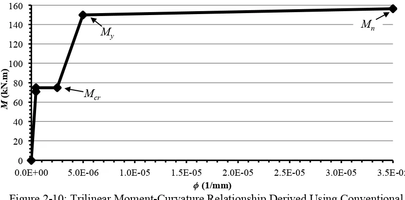
trilinear idealization of the moment-curvature relationship, shown in Figure 2-10, was

computed manually and using a MS Excel (2011) spreadsheet. The limits of the response

Increment εc

Choose c

Calculate Strain εs

Calculate Steel Stress & Force σs & Ts

Calculate Concrete Stress & Force σc & Cc

ΣF=0? Calculate Moment _Σ_M₌₀

Calculate Curvature ϕ

End of Loop

ΣF>0? N.A. Too Low;

Increase c

N.A. Too High; Reduce c

N

Y

(39)

are defined by the cracking, yielding and nominal ultimate moments, Mcr, My and Mn,

respectively, and the associated curvatures, ϕ.

Figure 2-10: Trilinear Moment-Curvature Relationship Derived Using Conventional Simplifying Approximations

Figure 2-11 shows the effective cross sections, strain distributions and stress distributions

assumed for the three phases of the trilinear idealization as follows:

• Linear-uncracked analysis – the applied moment is less than the cracking moment, Ma < Mcr. The section is therefore uncracked at this stage, as shown in

Figure 2-11(a). Transformed section properties were computed using the modular

ratio, n, which ranged from 31 at an age of 9.7 hours to 8.4 at an age of 28 days.

• Linear-cracked analysis – the applied moment exceeds the cracking moment but is less than the yield moment, Mcr ≤ Ma ≤ My. The section is now cracked, with the

concrete and steel exhibiting linear-elastic responses as shown in Figure 2-11(b).

The neutral axis depth in the uncracked section, kd, was calculated to satisfy

horizontal force equilibrium using Eq. [2.5]. Then the cracked moment of inertia 0

20 40 60 80 100 120 140 160

0.0E+00 5.0E-06 1.0E-05 1.5E-05 2.0E-05 2.5E-05 3.0E-05 3.5E-05

M

(

k

N

.m

)

ϕ(1/mm)

M_cr

(40)

was used to compute curvatures to satisfy moment equilibrium. The moment at which the steel yields (i.e. stress in the steel reaches fy) and the corresponding

curvature were also determined. The maximum concrete stresses was computed and compared to f0 from the experimental data to check the assumption of a

linear-elastic concrete response at steel yielding.

• Nonlinear-cracked analysis – the applied moment approaches the nominal ultimate capacity, Ma ≈ Mn. The equivalent rectangular concrete stress block

(41)

a) Linear-Uncracked Analysis

b) Linear-Cracked Analysis

c) Nonlinear-Cracked Analysis

Figure 2-11: Conventional Simplifying Approximations

The analysis highlighted the pitfalls of applying these simplifying approximations to very

young concretes. Figure 2-12 shows that, for 9.7-hour old concrete analysed using f0 and

Ec values from the Khan (1995) data, for the simplified trilinear idealization the

maximum concrete compressive stress at cracking is 0.66f0. At greater curvatures, the

assumption of a linear-elastic stress-strain relationship for concrete in compression is

doubtful, even for a reinforcement ratio of 0.5%. The computed maximum concrete

compression stress at steel yield greatly exceeds the compressive strength, so the

estimation of the yield moment using linear-elastic cracked section analysis is incorrect. b) Strain

b) Strain

a) Section c) Stress

ε_c ε_s σ_c σ_s ! ! kd

ε_cu

ε_s c

α1f'_c

σ_s ! β1c ! ! b) Strain

ε_c ε_s ! σ_c σ_s b) Strain b) Strain

ε_c ε_s σ_c σ_s ! ! kd

ε_cu

ε_s c

α1f'_c

σ_s ! β1c

! !

b) Strain

ε_c ε_s ! σ_c σ_s b) Strain b) Strain

a) Section c) Stress ε_c ε_s σ_c σ_s ! ! kd

a) Section c) Stress ε_cu

ε_s

c

α1f'_c

σ_s ! β1c ! ! b) Strain

a) Section c) Stress ε_c

ε_s

!

σ_c

(42)

The limit for c/d at ultimate is exceeded so the steel cannot be assumed to yield but

section failure is instead initiated by the concrete crushing in compression. Whitney

(1937) gives the following equation for the nominal moment of a section with

compression-initiated failure:

[2.12] Mn=0.333f'_cbd2

As shown in Figure 2-12(a), the nominal moment capacity obtained using this equation is

conservative.

a) 9.7h b) 14.5h

Figure 2-12: Moment-Curvature for Various Stress-Strain Relationships, ρ=0.5%

Figure 2-12(a) also shows the moment-curvature response computed from the Khan

stress-strain data (σc-εc, Khan), the Todeschini relationship (Tod.) and the Modified

Hognestad relationship (M. Hogn.). The shape of the moment-curvature response

computed from the Khan stress-strain data at an age of 9.7 hours, shown in Figure

2-12(a), differs from that of mature concrete. Because the steel stress never reaches yield,

the neutral axis depth, c, increases when the extreme fibre strain exceeds ε0, the strain

corresponding to the maximum concrete compressive stress. In the moment-curvature

0 10 20 30 40 50 60 70 80

0.0E+00 3.0E-06 6.0E-06 9.0E-06 1.2E-05

M (k N .m) ϕ (1/mm) 3-Stage M. Hogn. Tod.

σc-εc, Khan M_n, Eq. [2.12]

σ_c-ε_c, Khan

0 20 40 60 80 100 120 140 160

0.0E+00 1.0E-05 2.0E-05 3.0E-05

M (k N .m) ϕ (1/mm) 3-Stage M. Hogn. Tod.

(43)

analysis of a section containing mature concrete, the neutral axis depth, c, begins to

decreases after the steel yields.

Figure 2-12(b) shows the moment-curvature response when the concrete stress-strain

response corresponding to that observed by Khan (1995), at a concrete age of 14.5 hours.

In this case, the concrete has sufficient compressive strength to ensure steel yield at

ultimate, and the ultimate nominal moment computed from the CSA A23.3 (CSA 2014)

stress block idealization corresponds well to that computed from the observed

stress-strain data. Close agreement is observed for the moment-curvature relationships

computed from the observed stress-strain data reported by Khan, the Todeschini

relationship, the Modified Hognestad relationship and the conventional simplifying

approximations adopted in practice.

In both Figure 2-12(a) and (b), the moment-curvature relationships computed using the

concrete stress-strain data reported by Khan or the Modified Hognestad relationship are

similar, particularly in the region of maximum moment. The Modified Hognestad

relationship works well because it accurately models the descending branch of the

concrete stress-strain relationship observed by Khan as shown in Figure 2-6. The

moment-curvature response computed using the Todeschini relationship shows

significant strength loss beyond the maximum moment. As shown in Figure 2-13, the

depth of the compression region is required to be much larger to satisfy force equilibrium

using the Todeschini relationship. The resultant compressive force obtained assuming the

(44)

that obtained for the Modified Hognestad relationship. Hence the moment arm between

the resultant tension and compression forces is reduced, and so the resisting moment is

also reduced.

Figure 2-13: Force Equilibrium

Table 2-4 shows the variation of nominal ultimate moments and associated curvatures,

ϕn, computed for a beam with 9.7 hour-old concrete. The result using the conventional

simplifying approximations is based on a maximum concrete compressive strain of

0.0035 as specified in A23.3 (CSA 2014) with Mn computed using Eq. [2.12]. The

Todeschini relationship assumes strain softening for strains greater than ε0 so the nominal

ultimate moment occurs at a much lower curvature and smaller ultimate extreme fibre

compressive strain, εult. The Modified Hognestad relationship more accurately simulates

the observed descending branch of concrete in compression, Figure 2-6, and so yields a

Tensile Force Modified

Hognestad

Todeschini

Modified Hognestad Compressive Force

Todeschini Compressive Force

a) Stress Distribution b) Internal Forces

(45)

higher nominal ultimate moment and associated ultimate curvature that are close to those

computed using the concrete stress-strain data.

Table 2-4: Nominal Ultimate Moment and Curvature

Relationship εult ϕn (1/mm) Mn(kN.m)

Data, Khan 0.0044 11.2×10-6 _74.0

Conventional Simplifying

Approximations 0.0035 9.16×10-6 56.7

Todeschini 0.0013 4.35×10-6 _57.3

Modified Hognestad 0.0038 9.94×10-6 _71.0

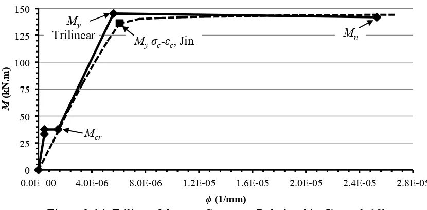
A similar result is obtained at a slightly older concrete age of 18 hours for a cross section

analyzed using the concrete stress-strain relationship observed by Jin et al. (2005), as

shown in Figure 2-14. The result obtained using the conventional simplifying

approximations provides a good approximation of the moment-curvature relationship

computed using the concrete stress-strain data reported by Jin et al. (2005). The yield

moment exceeds the ultimate nominal moment, however, even for a reinforcement ratio

of 0.5%. This solution is inadmissible because the calculated maximum concrete

compression stress corresponding to steel yield is 12.7MPa, exceeding f0 of 9.5MPa.

Using the observed concrete compression stress-strain data, the maximum concrete

compression stress corresponding to steel yield is 8.1MPa, and the associated yield

moment does not exceed the ultimate moment. Thus the conventional simplifying

approximations that are the basis of these methods don’t always hold for very young

concretes. The idealization of concrete in compression as a linear-elastic material to

(46)

limit, typically 0.6-0.7f0 (MacGregor & Bartlett 2000), let alone the compressive strength,

f0.

Figure 2-14: Trilinear Moment-Curvature Relationship, Jin et al. 18h

Figure 2-15(a) shows the effect of varying reinforcement ratio on the moment-curvature

relationships calculated for a section consisting of 9.7 hour-old concrete. As the area of

steel increases, the shortcomings of the Todeschini and Modified Hognestad relationships

are amplified. The higher reinforcement ratios cause the strain softening-deficiencies of

the Todeschini relationship to have an even greater impact on the nominal ultimate

moment. For all reinforcement ratios, use of the Todeschini and Modified Hognestad

relationships tend to overestimate the moments in the ascending portion of the

moment-curvature relationship because, as shown in Figure 2-6, both imply a greater secant

modulus than observed.

0 25 50 75 100 125 150

0.0E+00 4.0E-06 8.0E-06 1.2E-05 1.6E-05 2.0E-05 2.4E-05 2.8E-05

M

(

k

N

.m

)

ϕ(1/mm) M_cr

M_yσ_c-ε_c, Jin Mn

Short-term Deflections of Reinforced Concrete Beams

Scholarship@Western

Scholarship@Western

Short-term Deflections of Reinforced Concrete Beams

Short-term Deflections of Reinforced Concrete Beams

ABSTRACT

ACKNOWLEDGMENTS

TABLE OF CONTENTS

LIST OF FIGURES

LIST OF TABLES

LIST OF APPENDICES

NOMENCLATURE

CHAPTER 1:

INTRODUCTION

CHAPTER 2: EARLY-AGE CONCRETE

ε