A Method for Fast Establishing Tropospheric Refractivity Profile
Model Based on Radial Basis Function Neural Network
Tao Ma1, 2, Heng Liu1, 3, *, and Yu Zhang1, 3
Abstract—A method based on the radial basis function neural network (RBFNN) is developed to fast establish the tropospheric refractivity profile model. Parameters of the RBFNN include SPREAD, and the number of training samples is optimized. The actual measured data of meteorological station at Qingdao city in China are used as test data to evaluate the performance of RBFNN. The simulation results show that the root mean squared error (RMSE) has a minimum of 0.81 when SPREAD is 8.1. The simulated values agree well with the test data which is observed by using the sounding balloon method. Finally, the tropospheric refractivity profile model of a selected area is established by using two different simulation methods. This paper attempts to propose a method to fast establish the tropospheric refractivity profile model which provides an available method to correct the atmospheric refraction error in radar applications.
1. INTRODUCTION
Radar is widely used in the field of meteorological forecast, resource detection, environmental monitoring, and scientific research on celestial bodies, atmospheric physics, and ionospheric structures. It has been known that the radio wave refractive error caused by the inhomogeneity of atmospheric parameters, such as temperature, pressure and humidity, becomes a principal factor of influencing the high precision detection of radar. It is a significant approach to improve the detecting precision by using refractive error correction method. Hence, it is necessary to establish the atmospheric refractivity profile model in detecting area. The atmospheric parameters are obtained by the sounding balloon method which takes a lot of detecting time. Therefore, it is difficult to establish atmospheric refractivity profile model for anywhere quickly.
Simplified models based on a mass of historical detecting data have been studied extensively, for example, linear model, exponential model, double exponential model, Hopfield model, and subsection model [1–3]. A retrieval algorithm using ground-based global positioning system (GPS) is developed to establish the atmospheric refractivity profile model [4–6]. This method has high accuracy, but high searching volume and high time-consuming. An artificial neural network (ANN) is developed to estimate refractivity in the tropospheric region [7]. In ANN, sigmoid transfer function is used as the activation function between the hidden and output layers. The simulation results show that the relative humidity has more effect on the refractivity than other tropospheric parameters. The proposed ANN has a perfect capacity in estimating the tropospheric refractivity. Adding genetic algorithms (GAs) to the ANN, a hybrid model is introduced to solve the inversion problem of atmospheric refractivity estimation [8]. A very similar propagation factor curve with the reference one can be achieved by using the hybrid method. Recently, a radial basis function neural network (RBFNN) is used in many
Received 23 July 2019, Accepted 15 October 2019, Scheduled 30 October 2019
* Corresponding author: Heng Liu ([email protected]).
1 College of Electronic and Electrical Engineering, Henan Normal University, Xinxiang, China. 2 Key Laboratory Optoelectronic
research fields because of its excellent features, such as universal approximation, compact topology, and faster learning speed. Moreover, the RBFNN is basically an ANN with radial basis function as activation function, which has excellent nonlinear approximation capabilities [9–11]. Therefore, it is an important tool to solve problems which involve time series prediction, pattern recognition, and complex mappings. A study on time series prediction of a practical power system is developed by using RBFNN with a nonlinear time-varying evolution particle swarm optimization algorithm [12]. It is proved that the improved RBFNN has good forecasting accuracy, super convergence rate and short computation time in time series prediction for different electricity demands. The training algorithm and practical features of RBFNN are improved [13], and the RBFNN is used to control chart pattern recognition which can identify the classes by 99.63% accuracy. A RBFNN with K-Means clustering is also developed to establish the rainfall prediction model [14], estimate the sound source angle [15], and solve the problem of Direction of Arrival (DOA) [16]. To achieve accuracy traffic flow prediction, the artificial bee colony (ABC) algorithm is adopted to optimize weight and threshold value of RBFNN [17]. An improved RBFNN with gravitation search algorithm is proposed to predict network traffic which has perfect prediction accuracy [18]. In addition, the RBFNN is also used to increase the visibility of image [19] and classify the clinical medical signals for helping doctor identify the diseases [20, 21]. A prediction method based on RBFNN carries out not only the optimization of the microstrip line geometrical dimensions, but also characterization processes [22]. The RBFNN method is very accurate and extremely faster than the classical ones. It is also used to retrieve atmospheric extinction coefficients in the lidar measurements [23]. The results confirm that the model established by RBFNN is better than the Fernald method in the aspect of speed and robustness.
In this paper, a method based on RBFNN is proposed to fast establish the tropospheric refractivity profile. Principle of the RBFNN is introduced briefly. Then the tradeoff between the training time and
RMSE with increase of the training sample number is studied. The effect of SPREAD on RMSE is investigated, and an appropriate SPREAD is chosen for the following tropospheric refractivity profile model establishment. Afterwards, two different simulation methods using RBFNN are proposed to establish the tropospheric refractivity profile modal.
The rest of the paper is organized as follows. Section 2 describes the RBFNN model, including its principle and algorithm flow. The performances of the RBFNN and parameters optimization are discussed in Section 3. In Section 4, we establish and contrast the tropospheric refractivity profiles using two different simulation methods. At last, the conclusion is given.
2. RADIAL BASIS FUNCTION NEURAL NETWORK
Compared with the longer calculation and easily getting into local minimum of the back propagation (BP) neural network, the RBFNN can improve convergence speed and fitting performance significantly. The schematic diagram of the RBFNN is shown in Figure 1.
The RBFNN consists of three layers: input layer, hidden layer, and output layer. X = (x1, x2, ..., xN) is the input data set. N is the dimension of the input data set which is also the number
of input layers. Y = (y1, y2, ..., yM) is the M-dimensional output data set. H= (h1, h2, ..., hK) is the
neuron activation function of hidden layer, and K is the number of hidden neurons. In general, the neuron activation function of RBFNN is nonnegative nonlinear Gauss function:
hK = exp
−X−CK2
2σ2
(1)
whereCK(cK1, cK2, ..., cKN) andσ are the center and width of Gauss function, respectively. The input
data are directly fed to the hidden layers from input layers without any changes. Each output of the output layer is calculated using the weighted summation of the hidden neurons’ output:
ym=wmHT, m= 1,2, ..., M (2)
wherewm= [w1m, w2m, ..., wKm] denotes the weights of hidden neurons. The RBFNN is established by
training CK(cK1, cK2, ..., cKN),σ, and wm.
For simulating the atmospheric refractivity by using the RBFNN, Longitude (LONGITUDE), latitude (LATITUDE) and altitude (ATITUDE) of the observation stations are used as the input data which are expressed as matrixX= (LONGITUDE,LATITUDE, ATITUDE). The corresponding tropospheric refractivity (TROPOSPHERIC REFRACTIVITY) is the output which is expressed as
Y= (TROPOSPHERIC REFRACTIVITY, abbreviated asytr). Hence, the output of the RBFNN can
be expressed as
ytr=
K
i=1
wi1hi (3)
The center and Euclidean distance of the RBF affect the mapping ability of hidden layer neurons, which has a significant influence on the prediction data. In order to improve the accuracy and reduce the complexity of neural network significantly, the method of k-means clustering is used to choose the center appropriately [15].
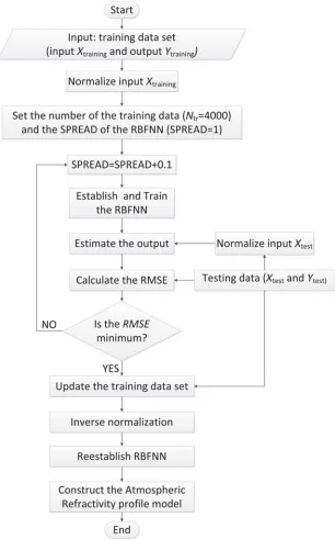
The implementation flow diagram (Figure 2) of the proposed RBFNN for establishing atmospheric refractivity profile model is as follows:
(1) Generating and normalizing the training data set (input Xtraining and output Ytraining) according
to the observation data of the meteorological stations.
(2) Setting initial values of the training data number (Ntr) and SPREAD, establishing and training
the RBFNN, optimizing the parameters (Ntr and SPREAD) by minimizingRMSE.
(3) Reestablishing the RBFNN and constructing the Atmospheric Refractivity profile model for the correction of TAR errors in the radar applications.
Here, the computer programs of thek-means clustering and RBFNN are performed on MATLAB (version 9.0.0.341360 [R2016a], Massachusetts, USA) environment. The training and simulation in this paper are done on a Lenovo computer with Intel core i7 and 16 GB RAM.
3. PERFORMANCE ANALYSIS AND PARAMETERS OPTIMIZATION
The data of meteorological stations at several Chinese cities, such as Zhengzhou, Qingdao, Guangzhou, Jiuquan, Shenyang, and Wulumuqi, are used in this paper. As we know, the refractive index of air (n) is ∼ 1.0003, which is represented as radio refractivity (or atmospheric refractivity, N) in radio band. Their relationship can be expressed in terms of Smith-Weintraub equation as follows [24, 25].
N = (n−1)×106 = 77.6Pd
T + 64.8 Pw
T + 3.776×10⁶ Pw
T2 (4)
Figure 2. The implementation flow diagram of the proposed method for establishing tropospheric refractivity profile model based on RBFNN.
The RBFNN is established and trained using the training data which are measured at the stations of Zhengzhou, Guangzhou, Jiuquan, Shenyang, and Wulumuqi. Then the measured data at Qingdao station are used as testing data to verify the performance of the RBFNN. RMSE is always used to evaluate the standard deviation between the actual value and predicted value.
RMSE =
Ntest
1
(ytr−yˆtr)2
Ntest
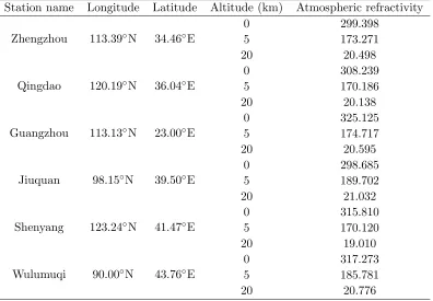
Table 1. Partial data used in this paper (in January 1, 1987).
Station name Longitude Latitude Altitude (km) Atmospheric refractivity
Zhengzhou 113.39◦N 34.46◦E
0 299.398
5 173.271
20 20.498
Qingdao 120.19◦N 36.04◦E
0 308.239
5 170.186
20 20.138
Guangzhou 113.13◦N 23.00◦E
0 325.125
5 174.717
20 20.595
Jiuquan 98.15◦N 39.50◦E
0 298.685
5 189.702
20 21.032
Shenyang 123.24◦N 41.47◦E
0 315.810
5 170.120
20 19.010
Wulumuqi 90.00◦N 43.76◦E
0 317.273
5 185.781
20 20.776
Figure 3. RMSE and training time (ttr) of the RBFNN with increase of the number of training data
(Ntr).
whereytr is the predicted value, ytr the actual measured value, and Ntest the number of testing data.
RMSE and training time (ttr) of the RBFNN are investigated as the number of training data (Ntr)
increases. The simulation results are shown in Figure 3. There is a great improvement of RMSE when the number of training data increases to 4000. ThenRMSE changes slowly. However,ttr exponentially
increases when the number of training data is greater than 8000. Therefore, the tradeoff betweenRMSE
and ttr must be considered.
(a) (b)
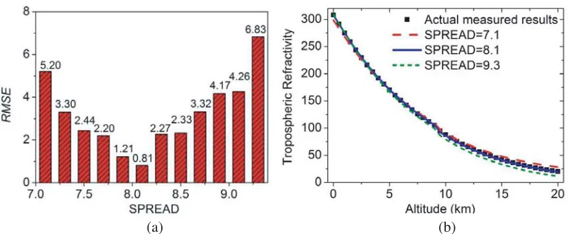
Figure 4. The optimization of SPREAD, (a) RMSE with different SPREAD and (b) tropospheric refractivity of Qingdao station with different altitude and SPREAD.
density [26]. It determines the number of hidden neurons, and then affects the smoothness of predicted output. The larger the SPREAD is, the smoother the function approximation is. Too large a SPREAD means that a lot of neurons are required to fit a fast-changing function. Too small a SPREAD means that many neurons are required to fit a smooth function, and the network might not be generalized well. Call RBF with different SPREADs to find the best value for a given problem. To optimize SPREAD, RMSE with different SPREAD is calculated and shown in Figure 4(a). From Figure 4(a), there is a minimumRMSE of 0.81 when SPREAD is around 8.1. Moreover, the simulated tropospheric refractivities with SPREAD of 7.1, 8.1, and 9.3 together with actual measured value are shown in Figure 4(b). The blue solid line (SPREAD = 8.1) is in the best agreement with the actual measured value. Hence, the SPREAD of 8.1 is chosen in the following simulations.
4. TROPOSPHERIC REFRACTIVITY PROFILE MODEL
China covers a vast geographic area. Its latitude and longitude range from 3.85◦N to 53.55◦N and from 73.55◦E to 135.08◦E, respectively. To establish the tropospheric refractivity profile model of China, the grid division method is always used to reduce the computation quantity of the algorithm. The modeling
(a) (b)
Figure 6. The schematic diagram of the method with updating training data (Method B).
(a) (b)
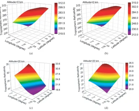
(c) (d)
region is divided into several grids. The tropospheric refractivity in each grid can be simulated based on the measured values of several nearby stations.
To verify this approach, the gray area (32.77◦N–42.77◦N, 103.26◦E–123.26◦E), which is shown in Figure 5(a), is chosen to establish the tropospheric refractivity profile model. The steps of latitude and longitude are 0.5 degrees and 1 degree, respectively. In Figure 5(a), the red star is the center of the 6 stations calculated by the K-means clustering. In this section, two methods are used to establish the tropospheric refractivity profile model in the gray area: one is the RBFNN without updating training data (denoted by Method A), and the other is the RBFNN with updating training data (denoted by Method B).
The tropospheric refractivity profile model is established using Method A, as shown in Figure 5(b). The tropospheric refractivity at an altitude of 0 km, 5 km, and 20 km ranges from 182 to 325.5, from 123.6 to 177.2, and from 17.2 to 40.5, respectively.
Meanwhile, another method with updating training data is also proposed to establish the tropospheric refractivity profile model. In this method, the grey area is divided into several layers, i.e., L1,L2, ..., L5, as shown in Figure 6(b), from the center labeled as the red star. For example, the
simulated results of layer L1 are added to the training data. Then the training data are updated before
the establishment of the layer L2, and so on in a similar fashion. In other words, the tropospheric
refractivity profile model is established according to the order of layers as shown by the red arrows in Figure 6.
The tropospheric refractivity profile models established using two different methods are shown in Figure 7. Comparing Figures 7(a), (b) and 7(c), (d), the relative deviation of atmospheric refractivity between two methods at an altitude of 20 km is less than that at an altitude of 0 km. The reason for the results is related to the different modeling processes of the two different methods.
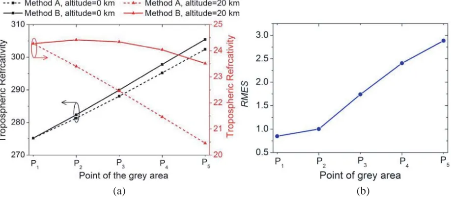
To make it easier to understand, 5 points at different layers in the grey area are chosen for comparison. Their tropospheric refractivities at altitudes of 0 km and 20 km are shown in Figure 8(a). At the beginning of modeling, the same tropospheric refractivity is achieved using the two methods. In this stage, the training data have not been updated yet. With the process of establishing the model which is fromP1 toP5 as shown in Figure 8(a), the deviation of results between two methods increases.
To evaluate the deviation during the simulation, the RMSE between two methods is calculated, as shown in Figure 8(b). FromP1 to P5, theRMSE increases from 0.85 to 2.88.
(a) (b)
5. CONCLUSION
A feasible method is proposed to fast establish the tropospheric refractivity profile model, which is based on the RBFNN with unsupervised learning. The simulation results demonstrate that the RBFNN is a fast and accuracy method for establishing tropospheric refractivity profile model. The methods with and without updating training data are proposed and compared during the modeling process. Their deviation increases from the inner layers to the outer layers. The profile model established by method with updating training data is smoother than that by the method without updating training data. The relationship between tropospheric refractivity and input parameters (longitude, latitude and altitude) can be achieved. The proposed method with updating training data is a promising approach for establishing tropospheric refractivity profile model. It provides a fast and convenient way for atmospheric refraction error correction.
ACKNOWLEDGMENT
This work is supported in part by the Scientific and Technological Project of Henan Province (182102310712), the Key Project of Henan Education Department (19A510002), and the Ph.D. Program of Henan Normal University (5101239170010).
REFERENCES
1. Salamon, S. J., H. J. Hansen, and H. D. Abbott, “Modelling radio refractive index in the atmospheric surface layer,”Electronics Letters, Vol. 51, No. 14, 1119–1121, 2015.
2. Bean, B. R. and G. D. Thayer, “Models of the atmospheric radio refractive index,” Proceedings of the IRE, Vol. 47, No. 5, 740–755, 1959.
3. Hopfield, H. S., “Two-quartic tropospheric refractivity profile for correcting satellite data,”Journal of Geophysical Research, Vol. 74, No. 18, 4487–4499, 1969.
4. Anthony, R. L., R. Chris, V. S. Sergey, and D. A. Kenneth, “Anderson vertical profiling of atmospheric refractivity from ground-based GPS,” Radio Science, Vol. 137, No. 3, 1–21, 2002. 5. Wu, Y. Y., Z. J. Hong, P. Guo, and J. Zhang, “Simulation of atmospheric refractive profile retrieving
from low-elevation ground-based GPS observations,”Chinese Journal of Geophysics, Vol. 53, No. 4, 639–645, 2010.
6. Chiou, M.-M. and J.-F. Kiang, “Retrieval of refractivity profile with ground-based radiooccultation by using an improved harmony search algorithm,” Progress In Electromagnetics Research M, Vol. 51, 19–31, 2016.
7. Ibeh, G. F. and G. A. Agbo, “Estimation of tropospheric refractivity with artificial neural network at Minna, Nigeria,”Global Journal of Science Frontier Research, Vol. 12, No. 1, 9–14, 2012. 8. Tepecik, C., and I. Navruz, “A novel hybrid model for inversion problem of atmospheric refractivity
estimation,” AEU — International Journal of Electronics and Communications, Vol. 84, 258–264, 2018.
9. Cai, Y., S. Sun, C. Wang, and C. Gao, “The research on flux linkage characteristic based on BP and RBF neural network for switched reluctance motor,” Progress In Electromagnetics Research M, Vol. 35, 151–161, 2014.
10. Adediji, A. T. and S. T. Ogunjo, “Variations in non-linearity in vertical distribution of microwave radio refractivity,” Progress In Electromagnetics Research M, Vol. 36, 177–183, 2014.
11. Lee, C. M. and C. N. Ko, “Time series prediction using RBF neural networks with a nonlinear time-varying evolution PSO algorithm,” Neurocomputing, Vol. 73, Nos. 1–3, 449–460, 2009. 12. Dubey, A. D., “K-Means based radial basis function neural networks for rainfall prediction,”
13. Addeh, A., A. Khormalib, and N. A. Golilarzc, “Control chart pattern recognition using RBF neural network with new training algorithm and practical features,” ISA Transactions, Vol. 79, 202–216, 2018.
14. Kumar, R., S. Srivastava, J. R. P. Gupta, and A. Mohindru, “Temporally local recurrent radial basis function network for modelingand adaptive control of nonlinear systems,”ISA Transactions, Vol. 87, 88–115, 2019.
15. Yang, X. P., Y. Q. Li, Y. Z. Sun, L. Teng, and T. K. Sarkar, “Fast and robust RBF neural network based on global K-means clustering with adaptive selection radius for sound source angle estimation,” IEEE Transactions on Antennas and Propagation, Vol. 66, No. 6, 3097–3107, 2018. 16. Zainud-Deen, S. H., H. A. El-Azem Malhat, K. H. Awadalla, and E. S. El-Hada, “Direction of
arrival and state of polarization estimation using radial basis function neural network (RBFNN),”
Progress In Electromagnetics Research B, Vol. 2, 137–150, 2008.
17. Chen, D. W., “Research on traffic flow prediction in the big data environment based on the improved RBF neural network,” IEEE Transactions on Industrial Informatics, Vol. 13, No. 4, 2000–2008, 2017.
18. Wei, D. F., “Network traffic prediction based on RBF neural network optimized by improved gravitation search algorithm,” Neural Computing and Applications, Vol. 28, No. 8, 2303–2312, 2017.
19. Chen, B. H., S. C. Huang, C. Y. Li, and S. Y. Kuo, “Haze removal using radial basis function networks for visibility restoration applications,” IEEE Transactions on Neural Networks and Learning Systems, Vol. 29, No. 8, 3828–3838, 2017.
20. Satapathy, S. K., S. Dehuri, and A. K. Jagadev, “EEG signal classification using PSO trained RBF neural network for epilepsy identification,” Informatics in Medicine Unlocked, Vol. 6, 1–11, 2017. 21. Kanojia, M. G. and S. Abraham, “Breast cancer detection using RBF neural network,”
International Conference on Contemporary Computing and Informatics, IEEE, Greater Noida, 2017.
22. Mohamed, M. D. A., E. A. Soliman, and M. A. El-Gamal, “Optimization and characterization of electromagnetically coupled patch antennas using RBF neural networks,” Journal of Electromagnetic Waves and Applications, Vol. 20, No. 8, 1101–1114, 2006.
23. Li, H. X., J. H. Chang, F. Xu, B. G. Liu, Z. X. Liu, L. Y. Zhu, and Z. B. Yang, “An RBF neural network approach for retrieving atmospheric extinction coefficients based on lidar measurements,”
Applied Physics B, Vol. 124, 184, 2018.
24. Smith, E. K. and S. Weintraub, “The constants in the equation for atmospheric refractive index at Radiofrequencies,”Proceedings of the IRE, Vol. 41, No. 8, 1035–1037, 1953.
25. Adediji, A. T. and M. O. Malhat, “Vertical profile of radio refractivity gradient in Akure South-West Nigeria,”Progress In Electromagnetics Research C, Vol. 4, 157–168, 2008.