Three Dimensional Electromagnetic Scattering of Two-Layer Rough
Surfaces Using Physical Optics Approximation Algorithm
Ke Li, Lixin Guo*, and Juan Li
Abstract—In this study, the physical optics approximation (POA) algorithm is described for predicting the electromagnetic (EM) scattering of three dimensional (3D) two-layer rough surfaces. The POA is initially used to calculate the composite scattering of an object and single layer rough surface under two dimensional (2D) situations. We extend this method to the case of a rough layer with two rough interfaces. The multiple coupling interactions between the upper and lower layer are considered based on an iterative strategy. Because the coupling effect is considered, the 3D model is quite time-consuming. In order to obtain numerical results rapidly, a parallel technique based on the OpenMP is adopted to accelerate the coupling iterative calculation. The model is applicable for moderate to large surface roughness. However, the rough surface should have small to moderate slopes so as to meet the conditions of POA. In numerical results, the normalized radar cross section of two-layer rough surfaces model under different polarizations is calculated, and the model is validated by comparison with a numerical reference method based on the method of moment. In addition, the influence of roughness on the scattering model is analyzed and discussed.
1. INTRODUCTION
Natural backgrounds, such as rough sea surface covered by insoluble oil, soil with snow on it, forest with layered vegetables, and all kinds of artificial material surfaces, are regarded as random rough surface models. Notably, most of the scenarios are layered rough surfaces. The scattering of these dielectric homogeneous layers is of significance in practical applications, such as surveillance to the soil, target tracking and navigation communication in complex backgrounds [1–3].
Theoretical simulation methods are always used to examine rough surfaces, and many methods have been developed to predict the EM scattering from rough surfaces or grating surfaces since the 1950s. In the open literature, several methods are used to examine the rough surface, such as the extinction theorem developed to calculate the scattering of rough surface and grating surface [4–6], a generalization of an integral theory used to calculate the enhanced backscattering from random rough surfaces [7], the Kirchhoff approximation (KA) [8, 9], the method of moments (MoM) [10], and a comprehensive approach of the forward-backward method (FBM) with spectral accelerate algorithm (SAA) combined with the physics-based two-grid (PBTG) method [11] which are investigated to calculate the scattering of rough surface. Notably, KA is extend to the high-order Kirchhoff scattering to examine the scattering of very rough 2D surfaces [12–15] and 3D surfaces [16, 17]. However, only a single layer is considered in these models. Meanwhile, the numerical methods consume a lot of computer resources, which limit their scope of application. Especially, if the layer rough surface is 3D model, the numerical methods seem insufficient because of the large calculation burden. Thus, the use of approximate models can be very efficient to predict the scattered field of 3D model systems. Many efficient approximate methods are investigated
Received 13 August 2018, Accepted 2 October 2018, Scheduled 15 October 2018 * Corresponding author: Lixin Guo ([email protected]).
to calculate these complex models, such as hybrid high-frequency shooting and bouncing rays-physical optics (SBR-PO) [18], hybrid KA-MoM algorithm [19], stabilized extended boundary condition method (SEBCM) [20], and modified equivalent current approximation (MECA) [21]. However, these works are either ineffective or not applied further on actual layered models. To date, several methods have been used to calculate the properties of layered rough surfaces or to analyze the polarimetric scattering from two-layer random rough surfaces with and without buried objects, such as rigorous numerical method multilevel fast multipole algorithm (MLFMA) [22], KA model [23], the steepest descent fast multipole method (SDFMM) [24], and geometrical optics (GO) models [25, 26]. Obviously, approximate methods can improve computational efficiency while maintaining the desirable precision.
In this study, a POA algorithm is developed for predicting the EM scattering of 3D two-layer rough surfaces. The POA is an extension of our previous work of physical optics with physical optics (PO-PO) [27, 28], and it is initially used to predict the scattering of a composite model which includes an object and a single rough surface. The aim of this work is to extend the PO-PO to the case of a two-layer rough surface. An iterative process is considered to calculate the coupling interaction between the upper and lower layer. The normalized radar cross section (NRCS) of the two-layer rough surfaces is calculated by using the proposed POA method, and the model is validated by comparing the results with those obtained from a numerical reference method based on MoM. In this study, the two-layer rough surface is modeled by using the Monte Carlo method with a Gaussian spectrum [29], and all fields and currents are assumed to have a time-harmonic dependence in the forme−iωt, which is suppressed in this study.
2. THE SCATTERING MODEL
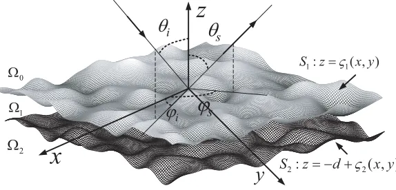
The geometry of the problem of interest is shown in Fig. 1. kˆi is the incident wave unit vector, and
ˆ
ks is the scattered wave unit vector. θi and ϕi are the incident elevation and azimuth angles, and θs
and ϕs are the scattered elevation and azimuth angles. The profile of the two-layered rough surface
divides the entire space into three spaces, and they are labeled as Ω0, Ω1, and Ω2. S1 denotes the upper layer surface with a profile ς1(x, y), and S2 denotes the lower layer with a profile ς2(x, y). S1 and S2 are generated by the Monte Carlo method, and they are uncorrelated. dis the average thick of the S1 layer. dmust be sufficiently large to avoid profile spatial overlap. The three spaces are characterized by relative permittivitiesεr0,εr1 andεr2, and they are assumed to be non-magnetic (relative permeability
μr0 =μr1=μr2= 1).
z
x
y
iθ
i
ϕ
sθ
s
ϕ
1: 1( , )
S z=ς x y
2: 2( , ) S z= − +d ς x y
0 Ω
1 Ω
2 Ω
Figure 1. Geometry of the problem: A 3D two-layer structure with rough boundaries.
Assume that the wave incident on the two-layer rough surfaces is a plane wave Einc(r) =
ˆ
eiexp(ik1·r), wherek1 =kkˆi is the incident wave vector;k=ω√μ0μr0ε0εr0;ε0 andμ0 are permittivity and permeability in free space;ˆei is the polarization direction of electric field vector.
of rough surface. In PO method, the fields at any point on the surface are approximated by the fields that would be present on the tangent plane at that point. Therefore, it is required that every point on the rough surface has a large radius of curvature relative to the incident wavelength so as to make PO valid [14]. However, it is always tedious to calculate the curvature radius of every point. For the scattering of rough surface only, PO method is also known as the KA method [9, 14], and the conditions of KA method [30] are expressed as
kl≥6, l2 >2.76δλ (1) where l is the correlation length, δ the root mean square (RMS) height of rough surface, and λ the incident wavelength.
On the basis of Huygens’ principle, the field at an observation pointr is expressed in terms of the fields at the boundary surfacer1. Thus, the scattered and transmitted fields at the two sides ofS1 are expressed as
Es(r) =
s1 ds1
ikη0GG(r,r1)·nˆ×H(r1) +∇ ×GG(r,r1)·ˆn×E(r1)
(2)
Et(r) =
s1 ds1
ik1η1GG1(r,r1)·ˆn1×H(r1) +∇ ×GG1(r,r1)·nˆ1×E(r1)
(3)
wherenˆ×E(r1) andnˆ×H(r1) are the total tangential electric and magnetic fields onS1;E(r) andH(r) are the total electric and magnetic fields in Ω0; ˆn and nˆ1 are the normal vectors to upper and lower surface of S1, respectively. Notably, nˆ1 =−ˆn. η0 =
μ0μr0/ε0εr0 is the intrinsic impedance in space Ω0, andη1=
μ0μr1/ε0εr1is the intrinsic impedance in space Ω1. k1=ω√μ0μr1ε0εr1,GG(r,r1) and
GG1(r,r1) are the space dyadic Green’s functions in Ω0 and Ω1, which are given by
GG(r,r1) =
II+ 1
k2∇∇
exp (ik|r−r1|) 4π|r−r1|
(4a)
GG1(r,r1) =
II+ 1
k21
∇∇
exp (ik1|r−r1|) 4π|r−r1| .
(4b)
To obtain the NRCS of the model, the accurately predicted total tangential electric and magnetic fields onS1 should be determined. In our POA method, an iterative process is considered to predict the scattering fields. Firstly, the primary values of ˆn×E(r1)|0 and ˆn×H(r1)|0 are set as the traditional POA tangential electric and magnetic fields on a plane patch [31], which they are zero in the non-lit region and are represented in the lit region as follows
ˆ
n×Er1
|0 =
ˆeT E ·Einc(r1) 1 +R01T E
(nˆ×ˆeT E)
−ˆeT M ·Einc(r1) 1−R01T M −ˆn·ˆki ˆeT E (5)
ˆ
n×Hr1
|0 = ˆeT E ·Einc(r1) 1−R01T E −nˆ·kˆi ˆeT E
+ˆeT M ·Einc(r1) 1 +R01T M
(ˆn׈eT E)
η0 (6)
where R01T E and R01T M are the local Fresnel reflection coefficients at S1 for the horizontal and vertical polarizations, respectively [32]. The number in the lower right corner represents the iterative order number. The superscript “01” indicates that the wave is incident in Ω0and refractive in Ω1, and it is an identity related to the space’s permittivity and permeability. For example,RT E10 indicates that the wave is incident in Ω1 and refractive in Ω0, andR12T E indicates that the wave is incident in Ω1 and refractive in Ω2. The permittivity and permeability appear in a fixed position of (2.1.49a) and (2.1.49b) in [32], and corresponding exchanges are made based on the identify “01”, “10”, or “12”. The locally defined unit vectors ˆeT E and ˆeT M to the upper surface of S1 are expressed as
ˆeT E = kˆi׈n
kˆi׈n ˆeT M =ˆeT E × ˆ
The combination of Eqs. (2), (3), (5) and (6) is the primary scattered field of upper layer rough surface. The shadowing regions must be taken into account based on the POA, and the shadowing is included in the calculation of POA tangential electric and magnetic fields explicitly by introducing functions inside Eqs. (5) and (6) in the form of geometric shadow functions:
s1(r1) =
1 ˆki·ˆn<0 (r1 is lit by incident wave) 0 ˆki·ˆn≥0 (r1 is not lit by incident wave)
(8)
Once the tangential fields expressed in Eqs. (5) and (6) are determined, the transmitted fields in Ω1 can be calculated by using Eq. (3). The tangential electric and magnetic fields onS2 are expressed as
ˆ n2×E
r2
|1 =
ˆ
e2T E·Et(r2) 1 +R12T E ˆn2׈e2T E
−ˆe2T M ·Et(r2) 1−R12T M
(−ˆn2·ˆr12)ˆe2T E (9)
ˆ n2×H
r2
|1 = ˆe2T E·Et(r2) 1−R12T E
(−nˆ2·ˆr12)ˆe2T E
+ˆe2T M ·Et(r2) 1 +R12T M nˆ2׈e2T E η1 (10)
where ˆn2 is the normal vector to S2,ˆr12= (r2−r1)/|r2−r1|. The locally defined unit vectorsˆe2T E andˆe2T M to S2 are expressed asˆe2T E =ˆr12×nˆ2/|ˆr12×nˆ2|andˆeT M2 =ˆe2T E ׈r12. Substituting Eq. (3) into Eqs. (9) and (10), the tangential electric and magnetic fields in lit-region on S2 can be written as
ˆ n2×E
r2
|1 =
s1 ds1
⎛
⎝ iωμη00μr1
1 +R12T EM+1−R12T MN
·(GG1(r2,r1)·K)
−1 +R12T EM+1−R12T MN
·[∇ ×GG1(r2,r1)·L] ⎞ ⎠
exp(ik1·r1) (11)
ˆ n2×H
r2
|1 = 1 η1 s1 ds1 ⎛
⎝ −iωμη00μr1
1−R12T EN −1 +R12T MM
·(GG1(r2,r1)·K) +1−R12T EN −1 +R12T MM
·(∇ ×GG1(r2,r1)·L) ⎞ ⎠
exp(ik1·r1) (12)
whereMand N are dyadics, andM,N,K, and L are given by
M=ˆn2׈e2T E
ˆ
e2T E, N = (nˆ2·ˆr12)ˆe2T Eˆe2T M (13)
K= (ˆeT E·ˆei) (ˆn·ˆr12)ˆeT E
1−RT E01 −(ˆeT M ·ˆei) (nˆ×ˆeT E)1 +RT M01
L= (ˆeT E·ˆei) (ˆn׈eT E)1 +RT E01 + (ˆeT M ·ˆei) (ˆn·ˆr12)ˆeT E
1−RT M01 . (14)
As Eq. (8), the shadowing of tangential electric and magnetic fields on S2 is also calculated by introducing functions inside Eqs. (9) and (10) in the form of geometric shadow functions:
s2(r2) =
1 ˆr12·nˆ2<0 (r2 is lit by scattered wave)
0 ˆr12·nˆ2≥0 (r2 is not lit by scattered wave) (15) On the basis of Eqs. (7)–(14), the tangential electricnˆ1×E(r1)|1 and magnetic fieldsnˆ1×H(r1)|1 in lit-region on the lower surface ofS1 radiated fromS2 can be obtained in an analogous manner. The expressions are given directly by
ˆ n1×E
r1
|1 =
ˆe1T E ·E 1 +RT E10 nˆ1׈e1T E
−ˆe1T M ·E 1−R10T M −ˆe1T E ·ˆr21
ˆe1T E (16)
ˆ n1×H
r1
|1 =
ˆ
e1T E ·E 1−RT E10 (−ˆn1·ˆr21)ˆe1T E+
ˆ
e1T M ·E 1 +RT M10 ˆn1׈e1T E
/η1(17)
E =
s2 ds2
ikη1GG1(r1,r2)·ˆn2×H
r2
|1+∇×GG1(r1,r2)·nˆ2×E
r2
|1
(18)
whereˆr21= (r1−r2)/|r1−r2|. The locally defined unit vectorsˆe1T E andˆe1T M to the lower surface of
As Eq. (8), the shadowing of tangential electric and magnetic fields on the lower boundary ofS1 is also calculated by introducing functions inside Eqs. (16) and (17) in the form of geometric shadow functions:
s3(r1) =
1 ˆr21·nˆ1<0 (r1 is lit by scattered wave)
0 ˆr21·nˆ1≥0 (r1 is not lit by scattered wave) (19) Thus, the newly updated tangential fields are expressed as
ˆ
n×Er1
|1 = nˆ×E
r1
|0 + ˆn1×E
r1
|1 (20)
ˆ
n×Hr1
|1 = nˆ×H
r1
|0 +nˆ1×H
r1
|1. (21)
Then,ˆn×E(r1)|1 and ˆn×H(r1)|1 are regarded as the primary tangential fields to calculate the secondary tangential fields onS2. At the same time, the secondary tangential fields on S1 are updated by the scattering fields fromS2. The total tangential fields onS1 are summations of all the high-order fields.
ˆ
n×Er1
=
m
1
ˆ
n×Er1
|n (22)
ˆ
n×Hr1
=
m
1
ˆ
n×Hr1
|n. (23)
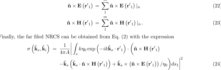
Finally, the far filed NRCS can be obtained from Eq. (2) with the expression
σ
ˆ
ks,kˆi = 1 4πA
skη0exp
−ikˆks·r1 ·
ˆ
n×Hr1
−ˆksˆks·nˆ×Hr
1 +ˆks×
ˆ
n×Er1
/η0
ds1
2 (24)
where m is the iterative steps. In our simulations we find that the total tangential fields on S1 are convergent after several steps, which in our simulation are set as 6. A is the projection area of rough surface on xoy plane in Descartes coordinate system.
3. NUMERICAL RESULTS
In the following numerical simulations, the EM scattering of two-layer rough surfaces is calculated and analyzed in detail by using the proposed POA method. All the simulations are obtained on a computer with a 3.4 GHz processor (Intel(R) Core(TM) i3-4130 CPU), 8 GB memory, and Intel Fortran compiler XE 13.0.
Numerical scattering results in incident plane under HH and V V polarizations are compared in Fig. 2. The relative permittivities of upper and lower layers are εr1 = 3.0 and εr2 =i∞ (PEC). The sizes of generated rough surfaces are 24λ×24λ. The root mean square (RMS) height and the correlation length in the numerical implementation are set toδ1=δ2= 0.1875λandl1 =l2 = 1.768λ, respectively. The average thickness of the upper layer rough surface is d = 2.41λ. The incident angles are set as
θi = 0◦ and ϕi = 0◦ for comparison to a numerical reference method based on MoM [25]. It is easily observed that the NRCS calculated by our POA method is in good agreement with that obtained by using the numerical reference method over the most angular range.
The model to be simulated below is described as follows. The relative permittivities of upper and lower layers are εr1= 3.0 and εr2 =i∞ (PEC). The average thickness of the upper layer rough surface is d = 5λ. Surface sizes of 24λ×24λ are simulated. The profiles of rough surface are generated as realizations of a Gaussian stochastic process with an isotropic Gaussian correlation function, and the correlation lengthsl=lx=ly are the same inxandydirections. The results are averaged by 50 Monte
Carlo realizations and observed in the scattering plane withθs=−90◦ ∼0◦ and ϕs = 15◦.
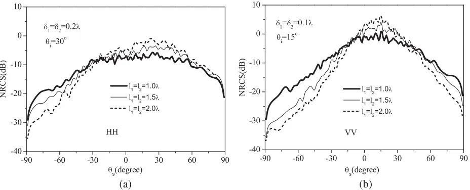
The effects of the correlation lengths on the NRCS of two-layer rough surfaces are depicted in Fig. 3. The incident angles are θi = 30◦ and ϕi = 0◦ for the HH polarization (Fig. 3(a)),θi= 15◦ and ϕi = 0◦
-90 -60 -30 0 30 60 90 -40
-30 -20 -10 0 10
l1=l2=1.768λ
NR
CS
(d
B
)
θs(degree) POA
HH
δ1=δ2=0.1875λ
Numerical Reference Method
-90 -60 -30 0 30 60 90
-40 -30 -20 -10 0 10
-90 -60 -30 0 30 60 90
-40 -30 -20 -10 0 10
l1=l2=1.768λ δ1=δ2=0.1875λ
NR
CS
(d
B
)
θs(degree) POA
VV
NR
CS
(d
B
)
θs(degree)
Numerical Reference Method
(a) (b)
Figure 2. Comparison of NRCS of two-layer rough surfaces under different polarizations (a) HH, (b)
V V.
-90 -60 -30 0 30 60 90
-40 -30 -20 -10 0 10
NR
CS(dB
)
θs(degree)
l1=l2=1.0λ
l1=l2=1.5λ
l
1=l2=2.0λ δ1=δ2=0.2λ
HH
θi=30 o
-90 -60 -30 0 30 60 90
-40 -30 -20 -10 0 10
θi=15 o
VV
δ1=δ2=0.1λ
N
RCS(
d
B
)
θs(degree)
l
1=l2=1.0λ
l1=l2=1.5λ
l1=l2=2.0λ
(a) (b)
Figure 3. NRCS of two-layer rough surfaces for different correlation lengths under different polarizations (a)HH, (b)V V.
δ1 =δ2 = 0.1λin Fig. 3(b) for both layers. The correlation lengths are set asl1 =l2 = 1.0λ,1.5λ,2.0λ. It can be seen that the NRCS increases with the increase of correlation lengths for different polarizations in the specular directions. The reason is that a large correlation length results in small RMS slope with the same RMS height. Thus, strong incoherent scattering can be observed as shown by the short dot line in Fig. 3. The scattering result in Fig. 3(b) varies more obvious than that in Fig. 3(b) in the directions far away from the specular directions, which indicates that the values of the scattering peaks are more sensitive to the variation in RMS length.
The effects of the RMS heights on the NRCS of two-layer rough surfaces are depicted in Fig. 4. The incident wave is the same as in Fig. 3. The correlation lengths are l1 =l2 = 1.5λin Fig. 4(a) and
-90 -60 -30 0 30 60 90 -50
-40 -30 -20 -10 0 10
NR
CS(dB
)
θs(degree)
δ1=δ2=0.05λ δ1=δ2=0.1λ δ1=δ2=0.2λ
HH
1
1=l2=1.5λ
θi=30 o
-90 -60 -30 0 30 60 90
-50 -40 -30 -20 -10 0 10
θi=15 o
NR
CS(dB
)
θs(degree)
δ1=δ2=0.05λ δ1=δ2=0.1λ δ1=δ2=0.2λ
11=l2=2.0λ
VV
(a) (b)
Figure 4. NRCS of two-layer rough surfaces for different RMS heights under different polarizations (a)HH, (b)V V.
Thread0
Thread0 Do i=1,18240
Thread1 Do i=18241,36480
Thread2 Do i=36481,54720
Thread3 Do i=54721,72692
Thread0 Serial region
!$OMP DO
Parallel region
Serial region
E X E C U T I O N
Figure 5. Graphical representation of the example explaining the general working principle of OpenMP.
Being an approximate method in evaluating EM scattering, the POA algorithm is valuable in actual applications, mainly benefited from its simple physical model, convenient mathematical formulation and computational efficiency, especially with the scenes of scattering from complex model. However, in this study POA is characterized by an iterative process for the two-layer rough surface, and the time-consuming computation effort still needs to be reduced. In order to obtain numerical results rapidly, a parallel technique based on the OpenMP [33] is adopted to accelerate the coupling iterative calculation. OpenMP is a new industry standard that has been created with the aim to serve as a good basis for the development of parallel programs on shared-memory machines. In our simulations, the graphical representation of the execution of OpenMP is represented in Fig. 5. The discretized unit dimension is
Table 1. The time-consuming of a two-layer rough surface for different CPU thread by the POA method for one realization in Fig. 3.
1 thread 2 threads 3 threads 4 threads
HH 1837.6 s 1120.8 s 848.2 s 727.9 s
V V 1855.2 s 1266.1 s 865.7 s 733.5 s
4. CONCLUSIONS
In this study, we extend POA to the case of a rough layer with two rough interfaces. The multiple coupling interactions between the upper and lower layers are considered based on an iterative strategy. The validation with a numerical reference method based on MoM shows that our method is effective. In numerical results, the EM scattering of two-layer rough surfaces model under different polarizations is calculated for different roughnesses of rough surface. The results indicate that the roughness of rough surface affects the scattering of two-layer rough surfaces remarkably. The study of 3D two-layer rough surface has engineering significance and practical value, and our method is effective for 3D problems; therefore, our method can provide theoretical reference for engineering applications.
ACKNOWLEDGMENT
This work was supported in part by the National Natural Science Foundation of China (Grant No. 61871457, Grant No. 61501360, Grant No. 61431010, Grant No. 41806210), and in part by the Foundation for Innovative Research Groups of the National Natural Science Foundation of China (Grant No. 61621005). The authors thank the reviewers for their helpful and constructive suggestions.
REFERENCES
1. Garcia, N. and E. Stoll, “Monte Carlo calculation for electromagnetic-wave scattering from random rough surfaces,” Physical Review Letters, Vol. 52, No. 20, 1798, 1984.
2. Kuga, Y. and P. Phu, “Experimental studies of millimeter-wave scattering in discrete random media and from rough surfaces,”Progress In Electromagnetics Research, Vol. 14, 37–88, 1996.
3. Ogilvy, J. A.,Theory of Wave Scattering from Random Rough Surfaces, Adam Hilger, Philadelphia, 1991.
4. Nieto-Vesperinas, M. and N. Garc´ıa, “A detailed study of the scattering of scalar waves from random rough surfaces,” Journal of Modern Optics, Vol. 28, No. 12, 1651–1672, 1981.
5. Garc´ıa, N. and A. A. Maradudin, “Exact calculations of the diffraction of S-polarized electromagnetic radiation from large-amplitude dielectric gratings,” Optics Communications, Vol. 45, No. 5, 301–306, 1983.
6. Nieto-Vesperinas, M. and J. M. Soto-Crespo, “Light-diffracted intensities from very deep gratings,”
Physical Review B: Condensed Matter, Vol. 38, No. 11, 7250, 1988.
7. Maystre, D. and M. Saillard, “Scattering from metallic and dielectric rough surfaces,” Journal of
the Optical Society of America A, Vol. 7, No. 6, 982–990, 1990.
8. Beckmann, P. and A. Spizzichino, The Scattering of Electromagnetic Waves from Rough Surfaces, Pergamon Press, 1963.
9. Thorsos, E. I., “The validity of the Kirchhoff approximation for rough surface scattering using a Gaussian roughness spectrum,”Journal of the Acoustical Society of America, Vol. 83, No. 1, 78–92, 1988.
11. Li, Z. and Y. Q. Jin, “Bistatic scattering and transmitting through a fractal rough surface with high permittivity using the physics-based two-grid method in conjunction with the forward-backward method and spectrum acceleration algorithm,” IEEE Transactions on Antennas & Propagation, Vol. 50, No. 9, 1323–1327, 2002.
12. Ishimaru and J. S. Chen, “Scattering from very rough surfaces based on the modified second-order Kirchhoff approximation with angular and propagation shadowing,”J. Acoust. Soc. Am., Vol. 88, No. 4, 1877–1883, 1990.
13. Chen, J. S. and A. Ishimaru, “Numerical simulation of the second-order Kirchhoff approximation from very rough surfaces and a study of backscattering enhancement,”J. Acoust. Soc. Am., Vol. 88, No. 4, 1846–1850, 1990.
14. Bruce, N. C. and J. C. Dainty, “Multiple scattering from rough dielectric and metal surfaces using the Kirchhoff approximation,” Optica Acta International Journal of Optics, Vol. 38, No. 8, 1471– 1481, 1991.
15. Bruce, N. C., A. J. Sant, and J. C. Dainty, “The Mueller matrix for rough surface scattering using the Kirchhoff approximation,” Optics Communications, Vol. 88, Nos. 4–6, 471–484, 1992.
16. Bruce, N. C., “Double scatter vector-wave Kirchhoff scattering from perfectly conducting surfaces with infinite slopes,”Journal of Optics, Vol. 12, No. 8, 526–526, 2010.
17. Bruce, N. C., “Multiple scatter of vector electromagnetic waves from rough metal surfaces with infinite slopes using the Kirchhoff approximation,” Waves in Random & Complex Media, Vol. 21, No. 2, 362–377, 2011.
18. Yang, W., C. Y. Kee, and C. F. Wang, “Novel extension of SBR-PO method for solving electrically large and complex electromagnetic scattering problemshould be a spacein half-space,” IEEE
Transactions on Geoscience & Remote Sensing, Vol. 55, No. 99, 1–10, 2017.
19. Ye, H. and Y. Q. Jin, “A hybrid KA-MoM algorithm for computation of scattering from a 3-D PEC target above a dielectric rough surface,”Radio Science, Vol. 43, No. 3, 2008.
20. Duan, X. and M. Moghaddam, “3-D vector electromagnetic scattering from arbitrary random rough surfaces using stabilized extended boundary condition method for remote sensing of soil moisture,”
IEEE Transactions on Geoscience &Remote Sensing, Vol. 50, No. 1, 87–103, 2012.
21. Gutierrez-Meana, J., J. A. Marti Nez-Lorenzo, and F. Las-Heras, “High frequency techniques: The physical optics approximation and the modified equivalent current approximation (MECA),”
Electromagnetic Waves Propagation in Complex Matter, 2011.
22. Qi, C. H. and Z. Q. Zhao, “Electromagnetic scattering and statistic analysis of clutter from oil contaminated sea surface,”Radioengineering, Vol. 24, No. 1, 87–92, 2015.
23. Tabatabaeenejad, A., X. Duan, and M. Moghaddam, “Coherent scattering of electromagnetic waves from two-layer rough surfaces within the Kirchhoff regime,” IEEE Transactions on Geoscience &
Remote Sensing, Vol. 51, No. 7, 3943–3953, 2013.
24. El-Shenawee, M., “Polarimetric scattering from two-layered two-dimensional random rough surfaces with and without buried objects,” IEEE Transactions on Geoscience & Remote Sensing, Vol. 42, No. 1, 67–76, 2004.
25. Pinel, N., J. T. Johnson, and C. Bourlier, “A geometrical optics model of three dimensional scattering from a rough layer with two rough surfaces,” IEEE Transactions on Antennas &
Propagation, Vol. 57, No. 2, 546–554, 2009.
26. Pinel, N., J. T. Johnson, and C. Bourlier, “A geometrical optics model of three dimensional scattering from a rough surface over a planar surface,” IEEE Transactions on Antennas &
Propagation, Vol. 57, No. 2, 546–554, 2009.
27. Li, J., L. Guo, and S. Chai, “Composite electromagnetic scattering from an object situated above rough surface,”Applied Optics, Vol. 53, No. 35, 8189, 2014.
29. Ji, W.-J. and C.-M. Tong, “The E-Pile+Smcg for scattering from an object below 2D soil rough surface,” Progress In Electromagnetics Research B, Vol. 33, 317–337, 2011.
30. Ulaby, F. T., et al., Microwave Remote Sensing: Active and Passive, Volume II: Radar Remote
Sensing and Surface Scattering and Emission Theory, Addison-Wesley Pub. Co., 1982.
31. Kouali, M., G. Kubicke, and C. Bourlier, “Electromagnetic interactions analysis between two 3-D scatterers using the E-PILE method combined with the PO approximation,” Progress in
Electromagnetics Research B, Vol. 58, 123–138, 2014.
32. Tsang, L. and J. A. Kong, Scattering of Electromagnetic Waves, Advanced Topics, Wiley Interscience, New York, 2001.
33. Chandra, R., L. Dagum, D. Kohr, D. Maydan, J. Mcdonald, and R. Menon, Parallel programming