R E S E A R C H
Open Access
Cross layer resource allocation for
fault-tolerant topology control in wireless mesh
networks based on genetic algorithm
Esmaeil Nik Maleki and Ghasem Mirjalily
*Abstract
Optimal topology control is an essential factor for efficient development of wireless mesh networks. For this purpose, a set of available tools can be exploited including power control, rate adaptation, channel assignment, channel selection, scheduling and routing. In most recent studies, only some of these tools are applied for throughput maximization. In this paper, we first propose a comprehensive cross-layer resource allocation model for topology control in which a complete set of available tools are exploited in order to guarantee the fairness, balancing and robustness, in addition to throughput maximization. This leads to an NP-complete problem; therefore, we propose a four steps heuristic method based on problem decomposition to reduce the computational complexity. In first step, the bestKpotential paths with disjoint vertices are extracted between each pair of nodes. In second step, a method based on the genetic algorithm is proposed in order to assign frequency channels to the links of these paths. This assignment procedure must preserve the essential links and must reduce the potential interference of the network. In third step, best compatible configurations are extracted on each frequency channel using power control and rate adaptation. It must be performed such that minimizes the power consumption, maximizes the transmission rate and provides the transmission rate balancing on the links. In last step, a cross-layer method is proposed for selecting the best path between each pair of nodes such that throughput maximization, fairness, and balancing on nodes and frequency channels are met. Validation in terms of numerical results demonstrates the efficiency of our proposed method for topology control in wireless mesh networks.
Keywords:Multi-radio multi-channel wireless mesh network, Resource allocation, Topology control, Genetic algorithm, Robustness against failures, Fairness, Balancing
1 Introduction
Recently, there is a growing interest in providing multi-media and wideband services on wireless networks. In this regard, wireless mesh networks have attracted much attention. These networks are classified as multi-hop networks and provide significant benefits including low-cost deployment, robustness and simple configur-ation [1–3]. In order to guarantee the quality of service in wireless mesh networks, the optimal resource alloca-tion and topology control is essential [4,5]. To this end, extensive research has been performed to modify the existing algorithms and to develop the novel algorithms.
1.1 Motivation
A wireless mesh network is composed of wireless mesh routers connected to each other by wideband connec-tions. Mesh routers are fixed nodes that play both the role of data routing and providing access points for net-work clients. With the development of technology, wire-less mesh routers are equipped with several radio interfaces capable of rate and power adjustment. Al-though, increasing the transmission power leads to the increasing transmission rate, it increases the interference and therefore, reduces the number of simultaneous
transmissions [3]. Moreover, several non-overlapping
channels are available in these networks where the effi-cient assignment of these channels to the radio
inter-faces results in throughput improvement [6, 7].
Consequently, the problem of trade-off between power
* Correspondence:[email protected]
Department of Electrical Engineering, Yazd University, Yazd, Iran
control and rate adaptation and efficient channel assign-ment must be addressed in wireless mesh networks. This procedure may result in more than one common chan-nel between two nodes producing a multi-graph top-ology for the network. Therefore, the proper selection of frequency channels is essential for increasing the net-work performance [8].
Since the number of frequency channels is limited, the simultaneous transmission on some links with the same channel is impossible. In order to reduce the co-channel interference, the power control and rate adjustment must be used. Moreover, the interfering transmissions can be scheduled on different time slots using a time-based scheduling algorithm. As a result, the optimal allocation of transmissions to the time slots along with the power control and rate adaptation is another problem that should be considered. Finally, the cross-layer routing to-gether with the layer-2 tools including channel assignment and selection, scheduling, power control and rate adapta-tion are essential for performance improvement. In most studies [4, 5, 9–17], only some of the available tools are exploited for efficient allocation of resources. Our pro-posed method includes a comprehensive set of tools to improve the network operation.
Based on the application of wireless mesh network, the objectives like throughput maximization, fairness between
traffic demands, balancing of frequency channels
utilization, and node utilization balancing must be consid-ered. However, only throughput maximization has been investigated in most researches [9–17]. This can result in some serious problems in the network. Firstly, because of the imbalance in resource utilization, the network con-gestion is occurred in some areas while the other areas carry low volume of traffic. Secondly, the fairness between traffic demands is not established and therefore, some traffic demands are not satisfied. Thirdly, the density of mesh routers is usually low and the traffic volumes are high; therefore, the failure of a router, even for a moment, greatly increases the packet losses. For this reason, in addition to the above-mentioned objectives, the robust-ness of the network against failures should also be consid-ered. According to the definition provided in [18], if the
network graph is K-Connected, the network will remain
connected even after the failure of fewer than K nodes.
Therefore, wireless mesh networks must be designed such that theK-Connectivity feature of the graph is guaranteed.
1.2 Methods
In this paper, we first introduce the problem of
Fault-Tolerant Topology Control with Throughput
Maximization, Balancing and Fairness (FTTC-TMBF) in which a comprehensive cross-layer resource allocation problem is modeled for topology control. In this model, a complete set of topology control tools are used
including power control, rate adaptation, channel assign-ment, channel selection, scheduling and routing. Here, we define the objective function with the aims of throughput maximization, frequency channel utilization balancing, node utilization balancing, fairness and ro-bustness against failures.
As it has been pointed out in [13, 14], the power
control in wireless mesh network is NP-complete. This issue is a subset of the topology control problem that has been studied in this paper; therefore, FTTC-TMBF is NP-complete and the computational complexity of FTTC-TMBF increases exponentially with any increase in the network size. In this paper, we propose the Heur-istic FTTC-TMBF (HFTTC-TMBF) method that is composed of four steps. In first step, we suggest an ap-propriate objective function to select the bestKdisjoint paths between each pair of nodes. This function mini-mizes the number of hops and the consumed power and also takes into account the node utilization balancing. In next step, the Genetic-Based Link Channel Assignment (GB-LCA) algorithm is proposed for assigning channels to links such that potential interference is minimized. In third step, we use the Genetic-Based Compatible Set Formation (GB-CSF) al-gorithm for extracting the set of common-channel links with minimum interference. For this purpose, power control and rate adaptation tools are employed and the cost function is minimized by using the genetic algo-rithm for each compatible set of links. Finally, we intro-duce the Genetic Based Cross Layer Paths Selection (GB-CLPS) algorithm, in which the best paths between each pair of nodes are selected by considering through-put maximization, fairness and balancing on frequency channels and nodes. The proposed algorithms of this paper is implemented in a centralized manner. Since the topology of wireless mesh networks are nearly fixed, the centralized implementation is a proper choice.
The rest of the paper is organized as follows.
Re-lated studies are reviewed in section 2. Section 3
de-fines the model and assumptions of the study. The cross-layer topology optimization problem is
formu-lated in section 4. The details of HFTTC-TMBF
solu-tion are provided in secsolu-tion 5. The simulation results
are analyzed in section 6. Finally, the paper is
con-cluded in Section 7.
2 Related work
In recent years, extensive research has been per-formed on cross-layer design of wireless mesh
net-works. In [9], the authors exploited the Mixed-Integer
it is a suitable choice to be compared with our
pro-posed approach. In [9], the optimization process is
di-vided in two phases. In the first phase, the authors find an optimum time-slot assignment for a scenario with a single shared channel, taking into consider-ation the routing. In the second one, starting from the first phase solution, a complete solution is built up for the multi-channel multi-radio scenario. Since this problem is NP-complete, a heuristic method based on the compatible configurations is proposed in which all the links that are feasible to transmit on the same channel at the same time are extracted. The
advantage of the model presented in [9] is its
com-pleteness because it considers all available tools and is the first complete model introduced in this field. However, its disadvantage is that its objective is only throughput maximization and it does not consider the balancing, fairness and robustness against failures that are very important in WMNs. In our proposed model FTTC-TMBF, we have added the balancing, fairness and K-connectivity feature to themodel intro-duced in [9]. In addition, we presented a four-step solu-tion where in first step, a heuristic method and in second to forth ones, a solution based on the genetic algorithm are used. In summary, we have proposed a comprehensive model in FTTC-TMBF to optimize the wireless mesh
networks in which the objectives of throughput
maximization, balancing, fairness and K-connectivity is considered, in addition to using all available tools; while, the model introduced in [9], only have considered the ob-jective of throughput maximization. Moreover, in
com-parison to [9], we have proposed HFTTC-TMBF in which
a heuristic method and genetic algorithm is used for solv-ing the problem.
In 2010, Luo et al. [10] developed two computational
tools for joint optimization of rate control, power con-trol, scheduling and routing. Moreover, they studied the relationship between frequency reuse and network per-formance as well as the benefits of multi-hop against single-hop. The tools developed by Luo et al. are based on the column generation and series solution of the problem, which produces the suboptimal solution in an acceptable time. In [9, 10], objectives such as fairness, balancing and robustness against failures are not considered.
In [11, 12], the authors exploited the MILP and
for-mulated the problem of gateway nodes selection along with the power control, routing and time slot assign-ment to maximize the service level of the nodes. They proposed a heuristic method to solve the prob-lem in a serial manner, which is composed of several steps. The issues of rate adaptation and channel
as-signment/selection are not considered in these
references.
Hedayati et al. [13], proposed a centralized
ap-proach to optimize the power consumption and rate adaptation with the aim of throughput maximization. They proposed a distributed version of their
algo-rithm in [14] where useful tools such as channel
as-signment and routing are not used. In [15], the
problem of robust topology control in multi-channel multi-radio wireless mesh networks is investigated. The authors formulated the problem in the form of a
Mixed-Integer Non-Linear Program (MINLP) to
maximize the end-to-end rate by considering the con-straints of routing, co-channel interference and fre-quency channel switching. In order to reduce the computational complexity of the problem, the authors proposed a heuristic method, which decomposes the problem, and then a binary search algorithm is used to find the sub-problem solution. However, some ob-jectives like fairness and balancing are not considered in any of the discussed references.
In [16, 17], the fairness objective is investigated in addition to the throughput maximization. The authors
in [16], developed a model and then solved it by using
the serialization method. In this reference, the network is assumed to be single-radio single-channel and single-rate; hence, the channel assignment and rate adaptation problems are ignored. In [17], differentiation among traffic flows is investigated such that the mini-mum fairness among different flows is guaranteed. This leads to the efficient distribution of bandwidth between clients. However, the effect of power control, rate adap-tation and channel assignment are not considered in this work.
In [19], we proposed a cross layer framework for the
optimal topology control where different tools such as power control, rate adaptation, scheduling, channel as-signment and routing tools have been used to achieve the goals such as throughput improvement and balan-cing. In this paper, robustness against failure and node utilization have not been modeled appropriately. More-over, the issue of fairness is not considered. In [20], we have represented a heuristic method for topology con-trol. However, some objectives like fairness and balan-cing have not been considered implicitly in this reference.
In [21, 22], the throughput maximization and
bal-ancing objectives are investigated. The authors in
[21] proposed a heuristic method by using the
chan-nel selection and rate adaptation tools. In [22], the
Due to the computational complexity of the cross-layer optimization problem, various meta-heuristic
methods have been proposed in recent studies [23–25].
In [23], a new routing method named MNSGA-II is
pro-posed in which a Genetic Algorithm (GA) procedure is used to extract the best paths with the aims of minimiz-ing the number of transmissions and delay. However, the other objectives and tools are not considered. In
[24], we proposed a GA-based method for power and
rate control along with scheduling in the wireless mesh networks. The objective function of this method only in-cludes the minimization of the number of time slots. Moreover, the routing and channel assignment are not
considered. The authors in [25] investigated multicast
routing and channel assignment problems simultaneously using a GA-based method in which power control and rate adaptation tools are ignored. In this method, the multicast trees are determined at first using differential evolution technique and then the channel assignment is performed by using a GA-based method. While the throughput maximization and fairness are considered in this reference, the balancing factor is not considered.
In [26–28], various methods of topology modification have been proposed in order to preserve the network ro-bustness against failures. The authors in [26] proposed a new protocol for topology control in wireless mesh net-work of hand-held devices. They selected a dominant set of interconnected nodes where the routing function is active in these nodes. This protocol results in the reduc-tion of collision, overhead, interference and energy con-sumption. However, the network is assumed single-channel, in which each node has a simple radio interface
with no rate and power adjustment capability. In [27],
Peng et al. proposed a linear network coding based fault-tolerant routing, which can recover the lost packets by the source. This method, by using multi-path routing and random linear network coding improves the con-ventional node selection methods. Another topology control method is investigated in [28], where the authors
have created aK-Connected graph based on the channel
assignment and routing. In these references, the authors have studied only some of the objectives which does not include the fairness and balancing.
Reviewing the previous references, it seems that pro-posing a comprehensive model for optimum resource al-location and topology control is still an open issue in wireless mesh networks. In this paper, we investigate the problem of topology control in wireless mesh networks which includes the following contributions,
A comprehensive cross-layer model for topology control problem is developed in which tools includ-ing power control, rate adaptation, channel assign-ment and selection, scheduling and routing are used.
A complete set of objectives such as throughput maximization, balancing and fairness is considered.
A decomposition-based heuristic method is pro-posed in order to reduce the computational com-plexity of the problem.
A new routing metric is introduced to determine the bestKpotential individual paths between node pairs based on theK-Connectivity feature
A channel assignment method based on the genetic algorithm is proposed to reduce the potential interference while preserves theK-Connectivity feature of the network
Genetic algorithm is used for power control and rate adaptation in order to determine the compatible links.
A heuristic method based on genetic algorithm is introduced for selecting the best path in order to provide fairness and balancing.
3 Network model and assumptions
In this paper, we model the network with a directed graph G= (V,E) where V= {v1,v2,v3,…,vn}represents n
nodes (wireless mesh routers) placed in a given area and
Edenotes the set of links between the nodes. In order to
determine E, the interference model should be defined.
In [29], two different interference models are introduced including the protocol interference model and physical interference model. The first model is specified with transmission range and interference range parameters in which all nodes in the transmission range of a given node can receive its messages correctly. In this model, if all messages are transmitted on the same frequency channel, the transmission on a given link can lead to interference on all links placed in the interference range of the transmitting node. The sufficient condition for the existence of a link between nodesiandjin the phys-ical interference model can be written asSINRij≥γ(ρ) in
which γ(ρ) represents a threshold level dependent on
transmission rate andSINRthat is defined as,
SINRij¼
HereN0is the thermal noise power,pijis the
transmis-sion power from node i to j, and Gij is the propagation
gain, such that Gij= (1/dij)ε, where ε is a parameter
dependent on the shadowing and fading phenomena and dijis the geometric distance between two nodes i and j.
Moreover, eij represents the link between two nodes i
and j. The second term of the denominator represents
must be greater than or equal toγ(ρ). In order to
calcu-late the denominator of SINRij, we ignore the effect of
links that the receiverjis placed outside the interference range of their transmitters [20].
Here, we assume that node iis equipped withIniradio
interfaces each has an omnidirectional antenna. Each
node transmits with one of the available rates R
= {ρ1,ρ2,…,ρM|ρ1<ρ2<. …<ρM}, and selects its
trans-mission power continuously from [0,Pmax]. Moreover,
one of the available non-overlapping frequency channels
Ω= {ωi|1≤i≤H}is assigned to each radio interface. In
order to prevent the intra-node interference, different channels must be assigned to radio interfaces of each node; this means that each node can simultaneously transmit on all of its radio interfaces. In this paper, we assume a schedule-based MAC protocol according to the TDMA with the maximum number of time slots in a time frame is represented byTmax. IfQis the set of node pairs which have the traffic request for transmission, then each traffic flow associated to the source and des-tination pair (u,v)∈Q is assumed to be unicast, where
TDuvrepresents the amount of traffic demand.
As mentioned before, robustness against failures
re-quires the network graph to be K-Connected. In [30],
Penrose proved that if the minimum degree of a network
graph isK, the network isK-Connected with high
prob-ability. Therefore, the minimum transmission power of each nodeiwith degreedegiis,
Pimin¼ min P ∈½0;Pmax degi≥K ;∀i∈V ð2Þ
In this paper, it is assumed that the network graph is po-tentially K-Connected in the condition of minimum
trans-mission rate and single frequency channel. Menger’s
theory says that there should beKpaths with distinct ver-tices between each pair of the nodes to guarantee the K-Connectivity feature of the network [31].
4 Fault-tolerant topology control with throughput maximization, balancing and fairness (FTTC-TMBF)
In this section, a comprehensive cross-layer model for topology control named FTTC-TMBF is introduced. In order to model the problem, some variables are defined as follows:
Xωijkt is a binary variable which is equal to 1 if at least one packet in time slottand frequency channelωis transmitted from nodeito nodejwith rateρk. Ptijis a real number from [0,Pmax] which shows the
transmission power of linkeijin time slott.
fuvijtrepresents the amount of traffic on link eijthat
belongs to the traffic session (u,v)∈Q in time slot t.
Table 1 summarizes all notations that will be used in
this section. By defining these variables, problem is for-mulated as follows.
In FTTC-TMBF, the objectives are throughput
maximization, fairness, balancing and robustness against failures; therefore, the objective function is:
Minimize α1
In the objective function (3), throughput maximization, fairness, nodes utilization balancing and frequency chan-nel utilization balancing are represented by four terms.
A- Throughput maximization - Since the matrix of
traffic demands is specified, the throughput
maximization is equivalent to minimizing the number of time slots in which the links are transmitting the data and is considered in first term of (3). In this equation, TNmax
a is the maximum number of time slots in which the
links are transmitting data.
B- Fairness between traffic flows -If only
maximiz-ing the total throughput is considered in the objective function, some sessions may receive the maximum ser-vice rate while the others get much less. In this paper, to provide fairness between traffic sessions, a satisfaction factor for each traffic session(u,v)is defined as (4),
SFuv¼
In order to provide fairness, the variance of satisfac-tion factor should be minimized. In (4),Cuv is the
aver-age capacity per time slot for the flow fromutovthat is defined as (5),
when TNuv is the maximum number of time slots in
which the flow from u to v is active. In (3), parameter
σ2;max
SF is the maximum variance of satisfaction factor and
σ2
SF is the variance of satisfaction factor as defined by (6),
σ2
where, |Q| represents the number of traffic demands in
between different traffic demands resulting from
SF¼P∀ðu;vÞ∈QSFuv=jQj.
C- Channel utilization balancing -When the
object-ive function only includes the fairness and throughput factors, the balancing in frequency channel utilization is severely affected. In other words, congestion may occur in one frequency channel, while the others carry a low volume of traffic. Therefore, minimizing the variance of channel utilization (σ2c) must also be considered in the objective function. For this purpose, we first define the amount of channel utilization as follows,
Uωc ¼
D- Node utilization balancing -Similar to the
balan-cing of frequency channel utilization, minimizing the vari-ance of node utilization (σ2
n) is also considered in the
objective function. The purpose of node utilization balan-cing is distributing traffic eventually across different nodes, but channel balancing means distributing traffic on different frequency channels. By defining the node utilization as (9), its variance is calculated from (10),
Ui
utilization for all nodes in the network. To adjust the importance of each of the four objective factors in (3), we use the coefficientsαi;i= 1,…, 4, where∑i= 1,…, 4αi
= 1. It is important to note that all of these objective fac-tors must be normalized before summation.
The constraints of FTTC-TMBF are shown below in eqs. (11) to (23). These constraints can be categorized in three classes: second layer constraints, third layer con-straints and cross-layer concon-straints. The second layer constraints are provided in (11) to (14). Eq. (11) shows the constraint of SINR for transmission on linkeijin
fre-quency channelω and time slottgiven that some other
links are active at the same frequency channel and the same time slot. The lower bound of transmission power
on each link is shown in (12). This quantity should be
higher than the minimum power required for transmitter Table 1List of some notations used in this paper
Notation Description
Ini Number of radio interfaces of nodei
R Set ofMavailable transmission rates
Pmax Maximum transmission power
Ω Set of non-overlapping channels chi Set of channels assigned to nodei
G Directed network graph
V Set ofnmesh routers
E Set of directed links
eij Directed link from nodeito nodej
Gij Propagation gain
dij Geometric distance between two nodesiandj
SINRij Signal to Interference and Noise Ratio in the receiver of linkeij γ(ρ) SINR threshold corresponding to the rateρ
N0 Thermal noise power
Pmin
i Minimum transmission power of nodeito satisfyK-degree requirement
Tmax Maximum number of time slots in a time frame
Pij Transmission power from nodeito nodej
degi Degree of nodei
TDuv The amount of traffic demand from source nodeuto
destination nodev
Xωt
ijk A binary variable which is equal to 1 if the transmission from nodeito nodejis scheduled in time slottwith frequency channelωand transmission rateρk
Pt
ij Transmission power of linkeijscheduled in time slott
fuvijt The amount of traffic belongs to traffic session (u,v)∈Qpassed on linkeijin time slott
Zuv
ijt A binary parameter which is equal to 1 iff uv ijt≻0
υ(ρk) The amount of transmitted traffic in one time slot at rateρk
Cuv End-to-end average throughput of traffic session (u,v)∈Q
in each time slot
SFuv Satisfaction factor for each traffic session (u,v)∈Q
σ2
SF Variance of satisfaction factor
SF Average satisfaction factor of all sessions
σ2;max
SF Maximum variance of satisfaction factor Ui
n Utilization of nodei
σ2
n Variance ofU i n
Un Average utilization of all nodes
σ2;max
n Maximum variance of node utilization Uωc Utilization of channelω
σ2
c Variance ofUωc
Uc Average utilization of all channels
σ2;max
node to beK-degree. Moreover, it should be higher than the minimum power required for a successful reception assumed no other link is active with the same frequency channel. The half-duplex property of each radio interface is represented in (13). According to (14), the maximum number of concurrent connections in a node is restricted to the number of its radio interfaces.
PtijGij≥γ ρk Xω
For third layer, the constraints of packet delivery
in end-to-end traffic flows are considered by
(15)–(18). Constraint (15) represents that the total traffic flow exported from the source node (or imported to the destination node) in every session must be equal to the amount of traffic demand at that session. As mentioned before, there should be
K disjoint paths between each node pair of set Q to
guarantee the K-Connectivity feature of the
net-work. This constraint is showed in (16)–(18), where
Zuv
ijtis a binary parameter which is equal to 1 if f
uv ijt
>0. Constraint (16) shows that the output traffic of
each source node routes to the K individual paths.
Similarly, (17) shows that the input traffic to each
destination node is delivered from K distinct paths.
Finally, (18) describes that the traffic between u
and v passes from a middle node no more than
once. These constraints guarantee the distinction of paths of each traffic flow.
X
The cross-layer constraints between network and MAC layers are expressed in (19) and (20). Constraint (19) rep-resents the relationship between variables of second and third layers. It implies that the total traffic transmitted on a link cannot be more than the maximum capacity of that link regarding the transmission rate, where υ(ρk)
repre-sents the amount of transmitted traffic in one time slot at rate ρk. Constraint (20) indicates that if some traffic
de-mands pass through a link, it should be active on at least one time slot with the assigned frequency channel and transmission rate. Finally, the variations of decision vari-ables are given in (21)–(23).
5 The proposed heuristic solution for FTTC-TMBF problem
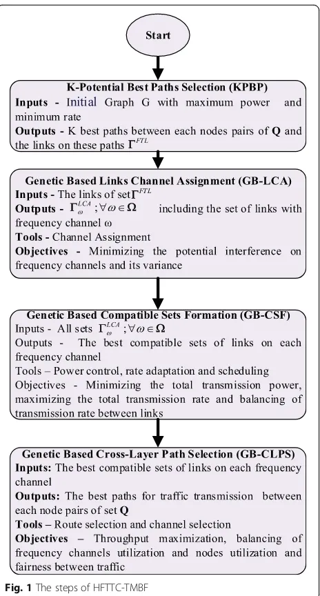
As mentioned before, the computational complexity of the proposed topology control problem is high. In order to reduce this complexity, we introduce HFTTC-TMBF which is based on decomposing the problem to four sub-problems including KPBP, GB-LCA, GB-CSF and GB-CLPS. The implementation of HFTTC-TMBF algo-rithm is shown in Fig.1. In this section, the
implementa-tion of these sub-problems is presented. Table 2
summarizes all notations that will be used in this section.
5.1 First step- K-potential best paths selection (KPBP)
With respect to the Menger theory, if a network graph is
K-Connected, then the graph should have Kpaths with
we have proposed KPBP in [20] which finds the best K
disjoint paths between each node pair of setQsuch that
the traffic delivery is guaranteed in the case ofK-1 fail-ures. In brief, the initial graph is formed based on the transmission with maximum power and minimum rate. Next, all of the vertices-disjoint paths between each
node pair of set Qare extracted. To this end, the
short-est path between the two nodes is obtained and all of the vertices and links of this path are removed. Then the second path is determined and removed from the graph. This procedure is continued until all paths are extracted. Finally using eq. (24) for each path, the best K paths be-tween nodes are obtained. Since in this step, no traffic demand is on the links, the proposed metric has poten-tially find K disjoint paths. This metric is a combination of the hop counts, power consumption for transmission on the links of the path and amount of usage from each
node in different paths. If the number of disjoint paths
and indices of nodes on thelth path between two nodes
u and v are shown by NoPuv and Pathuv, l ; l= 1, …,
NoPuv, respectively, then proposed cost function for
choosing the best K potential paths is formulated in
(24),
RCFuv;l¼α1H^uv;lþα2^Puv;lþα3B^uv;l ;α1þα2þα3¼1
;∀u;v∈Q;l¼1;2;…;NoPuv
ð24Þ
The first term of the cost function represents a generic routing measure which lead to the minimization of the number of hop counts. In (24), H^uv;l is the normalized
value of the number of hops on the lth path between
nodesuandvas defined in (25),
^
Huv;l¼ Path
uv;l
−1
Max∀10¼1;…;NoPuv Huv;l0
;∀u;v∈Q;l¼1;…;NoPuv
ð25Þ
Here,|Pathuv, l| indicates the dimension of the set
Pathuv, l, and the denominator shows the maximum
number of hops on different paths between two nodes used to normalize the number of hops.
If only the minimization of hop counts is considered, the paths with long hops are selected for data transmis-sion, which lead to increasing the power consumption of transmitters and consequently more interference. There-fore, power minimization must be considered in defining routing measure. If we show the total potential power
consumption of all links on thelthpath betweenuandv
withPsumuv;l, and the maximum potential power consump-tion of these links withPmax
uv;l, thenP^uv;lis defined
accord-ing to (26),
^ Puv;l¼
1 2
Psum uv;l
Max∀l0∈f1;2;…;NoPuvg P
sum uv;l0
þ1 2
Pmax uv;l
Max∀l0∈f1;2;…;NoPuvg P
max uv;l0
;∀u;v∈Q;l¼1;…;NoPuv
ð26Þ
In order to determine Psum
uv;l and Pmaxuv;l , the minimum
transmission power on each link must be calculated from (1), assuming no other link is active simultaneously and the transmission is performed using the minimum rate. In eq. (26), the denominators of the first and second terms show the maximum value of total power consumption for different available paths and the maximum power con-sumption of links for different paths, respectively.
In order to balance the node utilization, we prefer to use the paths that their vertices are less used on other paths. In this way, the normalized balance factor ^Buv;l is
Table 2List of notations used in HFTTC-TMBF
Notation Description
K-Potential Best Paths Selection (KPBP)
NoPuv Number of paths between two nodesuandv
Pathuv,l Indices of nodes on thelth path between two nodesuandv
^
Huv;l Normalized value of the number of hops on thelth path between two nodesuandv
Bnx
uv;l Number of usage of nodenxlocated on thelth path between nodesuandvon other paths
Psumuv;l Total power consumption of links on thelth path between two nodesuandv
Pmaxuv;l Maximum power consumption of links on thelth path between two nodesuandv ^
Puv;l Normalize power factor on thelth path between two nodesuandv
Bsumuv;l Total number of the usages of the nodes on thelth path between the two nodesuandvon other paths
Bmaxuv;l Maximum number of the usages of the nodes on thelth path between the two nodesuandvon other paths ^
Buv;l Normalized balance factor on thelth path between the two nodesuandv
RCFuv,ℓ Cost function of thelth path between nodesuandv ΓFTL
The set of required links to achieve aK-connected graph
|ΓFTL| Number of members in setΓFTL
Genetic Based Links Channel Assignment (GB-LCA)
Xgijωτ Gene in GB-LCA algorithm that is 1 if channelωis assigned to linkeijin generation g and chromosomeτ
Cgτ Chromosome in GB-LCA algorithm
Gg Generation population
PIgτ Potential interference on each chromosomeCgτbelonging to generationg
σ2;gτ
PI Variance of potential interference in each chromosome
PIgωτ Potential interference on each chromosomeCgτbelonging to generationgin frequency channelω
PIgmax Maximum potential interference among all chromosomes of generationg
σ2;gmax
PI Maximum variance of interference among all chromosomes of generationg COST(Cgτ) Cost function of chromosomeCgτ
Cgfa First parent (Father)
Cgma Second parent (Mother) Cgcτ Children chromosome
X
_gτ1
ijω Children gene
Cgmτ Mutation chromosome
μ Mutation rate
nm Number of chromosomes resulting from mutation
nμ Number of mutated genes
np Number of chromosomes in current generation
nc Number of children chromosomes
ΓLCA
ω Set of links with frequency channel ω∈Ω Genetic Based Compatible Sets Formation (GB-CSF)
Pgijτ Gene in GB-CSF that is the transmission power of each linkeijbelonging toΓLCAω
Sgτ Chromosome in GB-CSF algorithm
ρgτ
ij Transmission rate correspondent to geneP gτ ij
σ2;gτ
ρ Transmission rate variance of links in the chromosomeτ
ρgτ Transmission rate average of all links of the chromosomeτ Pgmax Maximum value of transmission power of the chromosomeτ
ρgmax
Maximum value of transmission rate of the chromosomeτ
σ2;gmax
^ Buv;l¼
1 2
Bmax uv;l
Max∀l0∈f1;2;…;NoPuvg B
max uv;l0
þ1 2
Bsum uv;l
Max∀l0∈f1;2;…;NoPuvg B
sum uv;l0
;∀u;v∈Q;l¼1;…;NoPuv
ð27Þ
For nodenxon the lth path between two nodesuand
v, if we show the number of its usage on other paths by
Bnx
uv;l, thenBmaxuv;l andBsumuv;l are defined as (28) and (29),
Bmaxuv;l ¼ Max∀nx∈pathuv;l B
nx
uv;l
;∀u;v∈Q;l¼1;…;NoPuv
ð28Þ
Bsum uv;l ¼
X
∀nx∈pathuv;l
Bnx
uv;l ;∀u;v∈Q;l¼1;…;NoPuv
ð29Þ
By applying the cost function (24) and extracting the
Kpaths between each pair of nodes, the set of required
links are achieved and stored inΓFTL.
Table 2List of notations used in HFTTC-TMBF(Continued)
Notation Description
COST(Sgτ) Cost function of chromosomeSgτ
Sgfa First parent (Father)
Sgma Second parent (Mother)
Sgcτ Children chromosome
P
_gτ1
ij Children gene
Sgmτ Mutation chromosome ~
Pgijτ Mutation gene
Genetic Based Cross Layer Path Selection (GB-CLPS)
Xguvkτ This gene is 1 ifkth path is selected for traffic flow of(u,v) Ρgτ Chromosome in GB-CLPS algorithm
LTτij Traffic on linkeijwhen all paths are selected based on chromosomeτ χij
uvl0 A binary parameter that is 1 if linkeijis onl’th path between nodesuandv
TNgωτm Number of time slots whenmth configuration set is active on frequency channelωin chromosomeτ
Γω
m Set of links belong tomth configuration set on frequency channelω
σ2;gτ
SF Variance of satisfaction factor of different traffic flows SFτuv Satisfaction factor of each traffic flow(u,v)
TNgsmax Maximum number of total time slots of all chromosomes
Cτuv Transmission rate of the link on the path fromutovwhich requires maximum number of time slots for transmission
pathτuv Set of links on the path selected between nodesuandvin chromosomeτ
σ2;gτ
n Variance of node utilization
σ2;gτ
c Variance of frequency channel utilization Vτa Set of active nodes in chromosomeτ
nτa Number of active nodes in chromosomeτ
Uτi Utilization of nodeiin chromosomeτ
Uτn Average of node utilization in chromosomeτ
Ωτ
a Set of active frequency channels in chromosomeτ
jΩτ
aj Number of active frequency channels in chromosomeτ Uτω Utilization of frequency channelωin chromosomeτ
Uτc Average of frequency channel utilization in chromosomeτ
Pgfa First parent (Father)
Pgma Second parent (Mother)
Pgcτ Children chromosome
X
_gτ
uvk Children gene
5.2 Second step- genetic based links channel assignment (GB-LCA)
In section 5–1, the set of essential links for preserving
the K-connectivity feature of the graph is extracted and
stored inΓFTL. In order to establish the
transmission/re-ception on each link of the set ΓFTL, there should be a
common channel between two end nodes of the link. In this section, the genetic algorithm is used for assigning a channel to these links considering the limited number of radio interfaces in each node. In other words, if the end
node i belongs to several links from set ΓFTLand the
number of radio interfaces ofiareIni, the total number
of frequency channels assigned to this node cannot be greater than Ini. In the following, required elements for
implementing GB-LCA are presented.
5.2.1 Genes, chromosome and population
In GB-LCA, the genes are assumed to be binary and rep-resented byXgτijω. In each chromosomeτfrom generationg, a gene takes the value of 1 if channelωis assigned to the linkeij. Chromosome is a set of genes that is defined asCgτ ¼ fXgτijωj∀eij∈ΓFTL;∀ω∈Ωg . Each chromosome has nv
= |ΓFTL| × |Ω| genes in which |ΓFTL| and |Ω| are
dimen-sion of setΓFTLand number of available frequency
chan-nels, respectively. Moreover, population is the set of np
chromosomes that are produced in each generation of the
algorithm implementation. The population of generationg
is shown byGg=〈Cgτ|τ= 1,…,np〉.
5.2.2 Cost function of GB-LCA
For each chromosome, the fitness functionF(Cgτ) is,
FðCgτÞ ¼α1
where,PIgτis the potential interference on each chromo-someτfrom generationg, which is defined as,
PIgτ¼ X
This function is the total potential interference on re-ceivers of all links inΓFTL. Moreover, σ2PI;gτ in (30) repre-sents the variance of potential interference on frequency channels in each chromosome. If potential interference on each frequency channel is defined as (32),
PIgωτ¼ X
then the variance of potential interference would be,
σ2;gτ
interference on all frequency channels. In (30), the
terms are normalized by using appropriate maximum values. In other words, denominators of first and sec-ond terms show maximum potential interference and maximum variance of interference between all chromo-somes of a generation, which can be obtained using (34) and (35), respectively.
To adjust the effect of each of the two objectives, we use the coefficientsαi;i= 1, 2 where∑i= 1, 2αi= 1.
The constraints of GB_LCA are defined in (36) and
(37). Equation (36) shows that a channel should be
assigned to each link of set.∀eij∈ΓFTL. Limitation on the
number of radio interfaces are given in (37). X
According to the definition of objective function (30) and constraints (36), (37), the cost function is defined as (38),
If the constraints (36) and (37) are established for each chromosome, COST(Cgτ)becomes equal toF(Cgτ); otherwise the cost of the assumed chromosome be-comes infinity. After introducing the concept of gene, population and generation, now the implementation steps of GB-LCA are described below. These steps in-clude the production of initial population, production and selection of next generation population, and the termination condition.
5.2.3 Production of the initial population
In order to produce the first-generation population G1,
common channel is assigned to one of the radio inter-faces of each node. We assign channels randomly to the remaining radio interfaces such that different radios on each node have different channels. By assigning fre-quency channels to the end nodes of each link of set
ΓFTL
, the genes of all chromosomes belonging to the first generation are initialized.
5.2.4 Next generation population
The potential population is produced by combining the chromosomes of the current generation, the children chromosomes, and the mutated chromosomes.
5.2.4.1 Children chromosomes An important part of
the genetic algorithm is to create a new solution called children. In order to produce the children chromo-somes, the chromosomes of the parents are extracted through tournament selection mechanism. In this
method, a set ofnfachromosomes from the current
gen-eration are chosen and the best one is selected as the first parent [32]. This parent is called father and denoted by Cgfa. The second parent (Cgma) is called mother and is obtained similarly. If we show the two chromosomes of ensuing children with Cgτ1
c and Cgτc 2, then each gene
of these chromosomes is produced using crossover oper-ator according to (39),
X _gτ1
ijω ¼ 1−ϑij
XgfaijωþϑijXgmaijω
;∀eij∈ΓFTL;∀ω∈Ω
X _gτ2
ijω ¼ϑijXgfaijωþ 1−ϑij
Xgmaijω
ð39Þ
The coefficientϑijis randomly selected as zero or one. In
addition, Xgfaijω and Xgmaijω are genes of the selected parents CgfaandCgma, respectively. This equation describes that the
channel assigned to linkeij(geneX _gτ1
ijω) is selected randomly
among channels assigned to this link in parent chromo-somes. Each time the crossover operator is run, two chro-mosomes are produced. In this problem, the number of children chromosomes is considered equal tonc.
5.2.4.2 Chromosomes resulting from mutation
Ran-dom variations of the chromosomes can decrease the time for achieving optimal solution. The mutation
op-erator implements these random variations in
GB-LCA. The resulting chromosome from the
muta-tion is shown by Cgτm. If the number of given
chromo-somes for mutation is denoted by nm, these
chromosomes are selected randomly among the chro-mosomes of the current generation.
In order to implement the mutation operator in each selected chromosome, the genes are first catego-rized based on the corresponding links. The set of genes related to link eijare denoted as Xgτijω ;∀ω∈Ω.
Therefore, the number of sets of genes is equal to
|ΓFTL| . If we denote the required mutation rate with
μ, nμ=⌈μ× |ΓFTL|⌉ sets must be selected randomly.
Then in each set and for each link eij, one of the
genes Xgτijω ;∀ω∈Ω is randomly set to 1 such that
constraint (37) is satisfied.
5.2.4.3 Choosing the population of next generation The next generation population includes three sets of current generation, the children chromosomes and the
mutated chromosomes. Figure 2 shows how population
of next generation is selected. If np, nc and nmrepresent
the number of current generation, children and mutants, respectively, then the number of potential members of the next generation population is equal tonp+nc+nm.
The number of chromosomes in each generation is equal tonp; therefore, some parts of the potential
popu-lation should be removed. To select the popupopu-lation of
next generation, the described three sets of
chromosomes are merged, and then np members with
less cost are selected according to the cost function (38).
5.2.5 Termination condition
We propose the following condition to stop execution,
ð40Þ
According to this equation, if the absolute value of the difference between minimum costs of the current and
previous generations is less than , the algorithm is
stopped. Then, the chromosomes with lower costs are chosen as the solution of the channel assignment prob-lem. Thus, by executing the GB-LCA algorithm,
fre-quency channels are assigned to the links of set ΓFTL .
This process can minimize the potential interference on each frequency channel, while at the same time satisfies the constraints (36) and (37).
5.3 Third step- genetic based compatible sets formation (GB-CSF)
In this section, we introduce the GB-CSF method for extracting all compatible sets. In each compatible set, the links can be active simultaneously without having interference on each other, such that minimizing the total transmission power and maximizing the total trans-mission rate is guaranteed. Moreover, the balancing of transmission rate between links is considered. GB-CSF algorithm is only implemented on the links with similar frequency channels; because other links with different frequency channels can be activated simultaneously without interfering with each other. If the links having
frequency channelω∈Ω are represented with ΓLCAω ,
GB-CSF is executed on each set of ΓLCAω iteratively. In
each execution on ΓLCAω , a set of links with lower cost are determined. Then these links are eliminated from
ΓLCA
ω and the algorithm is executed again on the
remained links. This procedure continues until no other link is remained in ΓLCAω . In the following, the execution procedure of GB-CSF for a specific set ΓLCAω is described. For other frequency channels, the same procedure is repeated.
5.3.1 Genes, chromosome and population
In this problem, genes are represented with Pgτij which
shows the transmission power of each linkeijbelonging to ΓLCA
ω . Therefore, gene is a continues variable that can take
a value in the interval [0,Pmax]. As mentioned before, a
chromosome is a set ofnv genes which is defined as Sgτ
¼ fPgτijj∀eij∈ΓLCAω g . The number of members of each
chromosome is equal to nv¼ jΓLCAω jwhere jΓLCAω jis the
dimension of set ΓLCA
ω . Moreover, the set of np
chromo-somes is produced in each generation g of the algorithm
implementation. This set is shown by Gg=〈Sgτ|τ= 1,…, np〉.
5.3.2 Cost function of GB-CSF
In this problem, the fitness functionF(Sgτ) is defined as (41),
In this equation, the first to third terms are related to the total transmission power, the total transmission rate on the links, and the transmission rate balancing in a chromosome, respectively. For every gene of a chromo-some, the corresponding transmission rate is deter-mined using (42),
which is the maximum rate of each link eijto satisfy the
SINR constraint. If this constraint is not satisfied for
minimum transmission rate ρ1, the given link cannot be
activated simultaneously along with other links. If the only objective is to maximize the transmission rate, some links might have the maximum transmission rate, while the others receive the minimum rate. For provid-ing the balancprovid-ing, variance of transmission rate should be as small as possible. In (41), σ2;gτ
ρ is the transmission
rate variance of links in the chromosome Sgτ of
gener-ationgdefined as,
σ2;gτ
mission rate for all links of the chromosomeτ. All terms
of (41) are normalized and then linearly combined using
appropriate coefficientsαi ; i= 1,…, 3such that∑i= 1,…,
3αi= 1 . The valuesPgmax,ρgmaxandσ2ρ;gmax represent the
maximum values of transmission power, transmission rate and variance of transmission rate, respectively.
These values are obtained using (44) and (45),
Pgmax¼ max∀τ′¼1;…;npðmax∀ei j∈ΓLCAω ðP
gτ′
i j ÞÞ
ρgmax¼ max
∀τ′¼1;…;npðmax∀ei j∈ΓLCAω ðρ
gτ′ i j ÞÞ
ð44Þ
σ2;gmax
ρ ¼ max∀τ′¼1;…;npðσ
2;gτ′
ρ Þ ð45Þ
According to the definition ofF(Sgτ), the cost function is defined in (46),
COSTðSgτÞ ¼ 1
FðSgτÞ ð46Þ
The implementation steps of GB-CSF include the pro-duction of initial population, propro-duction and selection of
next generation population, and the termination
condition.
5.3.3 Production of the initial population
In order to initialize the first generation, the transmis-sion power of genes that are available in all chromo-somes of the first generation should be determined. This power is selected randomly in the range ½Pgτij;min;Pmax,
where Pgτij;minrepresents the minimum power required for transmission with the minimum possible rate on linkeij
as-sumed no other link is active. This value is obtained as (47),
Pgijτ;min¼
N0γ ρð Þ1
Gij ;∀
eij∈ΓLCAω ;∀τ¼1;…;np
ð47Þ
5.3.4 Next generation population
As mentioned before, the potential population is pro-duced by combining the chromosomes of the current generation, the children chromosomes, and the mutated chromosomes. In the following, production of children chromosomes and mutated chromosomes are presented which are represented bySgτc andSgτm, respectively.
5.3.4.1 Children chromosomesIn order to produce the
children chromosomes, parent chromosomes Sgfa and
Sgmashould be selected first. To have a better search in the solution space, the parent chromosomes must be selected
randomly [33]. For this purpose, we use a roulette wheel mechanism based on the normalized fitness function,
PðSgτÞ ¼ F S
gτ ð Þ
Xnp
τ¼1
FðSgτÞ
;∀τ¼1;2;…;np
ð48Þ
In this method, a line with unit length is considered, and each segment of this line is assigned to each current
chromosome according to the value of P(Sgτ). In order
to select each parent chromosome, a random number with uniform distribution is produced in the range [0, 1]. Then the chromosome corresponding to the gener-ated random number is selected as the parent
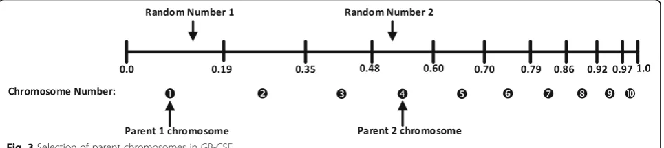
chromo-some. For instance, Fig. 3 shows how parent
chromosome is selected. In this figure, the values of
P(Sgτ) for chromosomes 1 to 10 is considered as 0.19,
0.16, 0.13, 0.12, 0.10, 0.09, 0.07, 0.06, 0.05, and 0.03, re-spectively. Based on these values, the length occupied by each chromosome is determined on the line. For select-ing a chromosome as a parent, the generated random number should be located in the region that is occupied by the corresponding chromosome. It is observed that in this method, a chromosome with higher fitness is more probable to be selected as a parent chromosome. More-over, the chromosomes with negligible probability are still possible to be selected; therefore, the variety of solu-tions is preserved.
If we show the two chromosomes of the ensuing chil-dren with Sgτ1
c and Sgτc 2; then, each gene of these
chro-mosomes is calculated according to (49),
P _gτ1
ij ¼ð1−ηÞP gfa ij þηP
gma ij
P _gτ2
ij ¼ηP gma
ij þð1−ηÞP gfa ij
: ð49Þ
in which Pgfaij and Pgmaij are the genes of the parents. According to (49), ifηis randomly selected in the range [0, 1], the children gens (transmission power levels) can never be outside the range of their parents. Therefore,
we define η in the interval −δ≤η≤1 +δ in which δ is
selected randomly using the uniform distribution in the interval [0, 1].
5.3.4.2 Chromosomes resulting from mutation If the resulting chromosome from the mutation is shown by Sgτm, the number of mutated genes in this chromosome is
determined based on the mutation rateμ which reflects
the percentage of variation in the genes. In order to pre-serve the historical memory of the algorithm, the new power levels (mutated genes) must be produced in a way that they are placed in the neighborhood of the selected chromosomes for mutation. Therefore, we use the nor-mal distribution for the mutation operator. There are a
lot of references such as [34–36] in which the normal
distribution is used for mutation operator. Without loss of generality, we assume that the genePgτij from
chromo-someSgτis randomly selected for mutation. The mutated
gene is defined according to (50),
~
Pgijτ¼PgijτþεNð0;1Þ ð50Þ
in whichN(0,1)is the normal distribution function with
zero mean and unit variance. At the beginning, εis
con-sidered in the range[0,Pmax]. After applying the mutation operator, this parameter is modified according to (51),
εnew¼ minP
The successful percentage of mutation is the number of mutant chromosomes that their cost is reduced com-pared to the original chromosome. In the above equa-tion,℘is an arbitrary threshold.
5.3.4.3 Choosing the population of next generation
Similar to the proposed method in 5–2-4 for GB-LCA,
at first all chromosomes of current population, children chromosomes and mutation chromosomes must be
merged and then npmembers with lower cost are
se-lected as population of the next generation. Therefore, in this method, the best chromosomes of each gener-ation are transferred to the next genergener-ation and the his-torical memory of the algorithm is preserved.
5.3.5 Termination condition
In order to stop the algorithm, the absolute value of the difference between minimum costs of the current and
previous generations should not be higher
than the threshold. In other words, the termination
con-dition is similar to (40) in which the name of current
generation chromosomes and previous chromosomes are replaced with Sgτand S(g−1)τ, respectively. Here, the chromosomes with lower costs are chosen among the current generation chromosomes. Then, the links of this
chromosome are eliminated from the set ΓLCAω and the
procedure of extracting the compatible sets continues
until set ΓLCA
ω is emptied. The algorithm is repeated for
other sets.
5.4 Fourth step- genetic based cross-layer path selection (GB-CLPS)
In this section, we introduce a Genetic Based
Cross-Layer Path Selection (GB-CLPS) algorithm that uses path and channel selection tools to fulfill the goals such as balancing and fairness. As explained earlier in sections 5–1 to 5–3, first, theKbest potential paths be-tween node pairs were extracted in step 1 using KPBP; then in step 2, the best channels were assigned to links of these paths using GB-LCA. In step 3, the best com-patible sets of links on each frequency channel were ob-tained using GB-CSF. GB-CLPS algorithm selects the best
path for transmission among K selected paths between
each node pair such that not only throughput is maxi-mized, but also balancing of frequency channels utilization and nodes utilization and fairness between traffic flows are provided. For this purpose, path and channel selection tools based on genetic algorithm are used.
5.4.1 Genes, chromosome and population
A gene is a binary value denoted byXgτuvk that is equal to 1 if the kth path is selected for traffic flow (u,v). A chromosome is the set of genes that can be defined as
Ρgτ¼ fXgτ
uvkjðu;vÞ∈Q;k¼1;2;…;Kg, where the number
of genes in the chromosome is equal to nv= |Q| ×K.
Population is the set ofnpchromosomes of the problem.
5.4.2 Cost function of GB-CLPS
By determining each chromosome, paths between each
node pairuandvbelong to setQare determined. Traffic
on each linkeijof the network is calculated as (52),
where,χijuvl0is a binary parameter that is equal to 1 if link eij is on the l′th path between nodesu and v. For each
chromosome, the cost function COST(Pgτ) is defined
with (53),
objective, coefficientsαi ;i= 1, .., 4 are used, where∑i= 1,
.., 4αi= 1. The first term of the cost function shows the
total time slots required for traffic transmission. Since the transmission rate of each link is obtained using GB-CSF, the maximum throughput is achieved by minimizing the number of time slots required for traffic transmission. In (53),NoSωis the number of available configuration sets for
frequency channelω, which is obtained from GB-CSF. In
addition,TNgτωmthat is the maximum number of used time
slots when the mth configuration set is active on
fre-quency channelω, is obtained using (54),
TNgωτm¼ max∀eij∈Γω frequency channelω. In addition, ρijis the transmission
rate of link eijthat is obtained from GB-CSF, and T
rep-resents the length of each time slot. In order to calculate
TNgτωm, the maximum number of time slots required for
transmitting traffic flows on each link of a configuration set should be obtained.
For fairness, the variance of satisfaction factors of dif-ferent traffic flows (σ2SF;gτ) defined in (55) should be
factor of service for each traffic flow (u,v) where Cτuv is the transmission rate of the link on the path that re-quires the maximum number of time slots for transmis-sion. The amount ofCτuvis calculated from (56),
in which pathτuvis the set of links on the selected path
between nodesuandvin chromosomeτ. In addition, in
(55), SFτ ¼P∀ðu;vÞ∈QSFτuv=jQjis the average of
satis-faction factors of all traffic flows.
In order to provide balancing, variances of node utilization (σ2n;gτ) and frequency channel utilization (σ2c;gτ) should be minimized.σ2;gτ
n is defined as follows,
σ2;gτ ber of active nodes in chromosomeτth. An active node is a
node with non-zero traffic. Uτi and Uτnare the amount of
node i utilization and average of node utilization in
chromosomeτwhich are defined in (58) and (59),
Similarly, the variance of channel utilization (σ2;gτ c ) is
obtained using (60),
σ2;gτ channels and the number of active frequency channels
in chromosome τ. An active channel is a channel in
which its traffic load is not zero. In addition, the utilization and average utilization of each frequency channelωare defined in (61) and (62),
the maximum values of total numbers of time slots, variance of satisfaction factor, variance of node utilization and vari-ance of channel utilization between all chromosomes, re-spectively. These values can be obtained using (63) to (66), respectively,
5.4.3 Implementation of GB-CLPS
GB-CLPS is based on the implementation of a binary
implementation steps: production of the initial popula-tion, production and selection of next generation popu-lation, and the termination condition. In order to produce the first-generation population, we randomly assign 0 or 1 to each gene in a chromosome. In each chromosome, one path between∀(u,v)∈Qshould be se-lected. The potential population of the next generation is formed from the population of chromosomes in the current generation i.e.Pgτ ;τ= 1,…,np, mutation
chro-mosomes and children chrochro-mosomes.
In order to produce the children chromosomes, the chro-mosomes of the parents are extracted through tournament
selection mechanism. In this method,nfachromosomes are
selected from the current generation for the first parent (father). These chromosomes are selected among current generation chromosomes according to the cost function. The second parent (Pgma) is obtained similarly. Each of the genes in the two children chromosomes obtained from the crossover operator by using eq. (67),
X_guvkτ1¼ð1−ϑuvÞXgfauvkþϑuvXgmauvk ;∀ðu;vÞ∈Q;∀k¼1;…;K
X_guvkτ2 ¼ϑuvXuvkgfa þð1−ϑuvÞXgmauvk
ð67Þ
where the coefficientsϑuvare randomly selected as zero
or one. Therefore, each time the crossover operator is
run, two chromosomes (Pgτ1
c and Pgτc 2) are produced. In
this problem, the number of children chromosomes is
considered equal to nc. As mentioned before, random
variations of chromosomes are performed by using mu-tation operator. A chromosome produced by mumu-tation is
shown byPgτm. The number of chromosomes selected for
mutation is denoted by nm. In order to implement the
mutation operator, we define the set of gens correspond-ing to each traffic flow (u,v)as Xgτuvk ;∀k¼1;…;K. If
the required mutation rate is equal to μ, nμ=
⌈μ× |Q|⌉set of gens is randomly selected at first. Then in each selected set and for every traffic flow(u,v), one of the genesXgτuvk ;∀k¼1;…;Kis randomly set to 1.
In order to select the next generation population, the three sets of chromosomes including current population, children chromosomes and mutation chromosomes are
combined and np members are selected according to
their costs. The termination condition is similar to the
(40) where the chromosomes are replaced by Pgτ, and
the cost function is similar to (53). After the termination condition is met, the chromosomes with lower cost will be selected among the current generation of chromo-somes. Thus, the best paths for traffic transmission are selected by considering throughput, balancing and fair-ness factors.
6 Experimental results and discussion
In this section, we evaluate the performance of FTTC-TMBF and HFFTC-TMBF methods using some different scenarios. In each scenario, a number of wire-less mesh routers is randomly distributed in a given area. Each router is equipped with at most three advanced radio interfaces that can adjust the transmission power
in the range [0,Pmax] with Pmax equal to 20dbm. They
also can use different transmission rates using different coding and modulation schemes. In order to have a suc-cessful reception, the SINR level of the receiver must be higher than the threshold value. According to IEEE 802.11a standard, different values of transmission rates including 6, 9, 12, 18, 24, 36, 48 and 54 Mbps are avail-able for each interface and the SINR threshold corre-sponding to these values are 6.02, 7.78, 9.03, 10.79, 17.04, 18.8, 24.05 and 24.56 dB, respectively [37].
It is assumed that the maximum number of available non-overlapping frequency channels that can be assigned to radio interfaces is 12. Moreover, according to [13, 14], the interference range and the parameterεof the propaga-tion gain are set to 350 m and 2.5 respectively, unless other-wise specified. Here, the noise power is set to N0=−90
dBm, and the connectivity number K is set to 2. In
addition, the weight coefficientsαiof the objective and cost
functions are assumed equal, unless otherwise specified. Each point on the result graphs is the average obtained from 100 simulation runs. In this paper, we used MATLAB as simulation tool and GAMS as optimization solver.
6.1 Simulation and analysis of FTTC-TMBF
In this section, we compare the solution of the FTTC-TMBF model with the algorithm introduced in
[9]. We assume that the nodes are randomly distributed
in a square area of 1km2. Also, ten traffic demands is
considered for the network where the volume of each traffic flow is randomly selected between 15 and 30 MB.
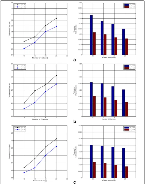
In Fig.4, the performance of the FTTC-TMBF solution
with objective function (3) and coefficientsα1= 2/5,αi=
1/5; i= 2, 3, 4 is compared with the solution introduced
in [9]. As seen from Fig.4a, the network throughput of
FTTC-TMBF is lower as compared to the [9]. This is
be-cause in [9], the fairness and balancing are not consid-ered in the objective function and the optimization is done only with the aim of throughput maximization; while, our proposed model considers a complete set of objectives including throughput maximization, fairness, balancing and robustness against failures. Moreover, by increasing the number of nodes, throughput is increased. This is because the links length is decreased and accord-ing to the power control ability of the algorithms, less power is required for successful transmission; therefore, the interference is decreased and throughput is
10–20 for the algorithm in [9] and in interval n = 10–15 for FTTC-TMBF. With further increase in the number of nodes, the throughput continues increasing as ex-plained above, but because the nodes become very close to each other, we reach the minimum transmission power and from this point, the power control stops re-ducing the transmission power. As a result, by increasing the number of nodes beyond a threshold, the interfer-ence is increased significantly. In this case, although the received power is also increased, because of the dense nodes and high interference, the throughput increase slope is reduced.
Figure 4b represents the variance of node utilization
in FTTC-TMBF, which is decreased compared to [9].
This parameter is decreased as the number of nodes is increased, because the fair distribution of traffic is more possible by having more nodes in the network.
The comparison between the variance of channel
utilization is depicted in Fig. 4c when the number of
nodes is set to 20. It shows that the frequency chan-nels are used more uniformly in FTTC-TMBF. More-over, the utilization of the channels is more uniformly as the number of frequency channels is increased, which is due to the better traffic distribution among different channels. Finally, Fig. 4d shows that the
vari-ance of satisfaction factor is decreased in
FTTC-TMBF, which means the fairness between dif-ferent traffic flows is improved.
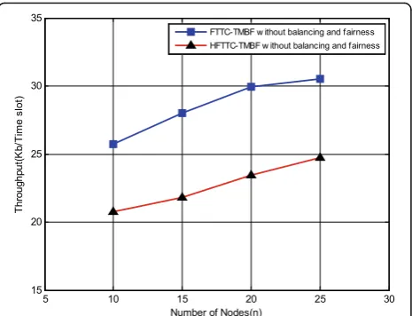
The impact of balancing and fairness factors on the
throughput has been investigated in Fig. 5. It is
shown that the variance of node utilization is de-creased by increasing the effect of this factor in ob-jective function (increasing coefficient α3 in (3)). Also, by increasing the number of nodes, the throughput is
a
b
c
d
a
b
c
increased because due to the reduced length of links and lower transmission power for data transmission, more links are active simultaneously. It is also evident
from Fig. 5a that by increasing the number of nodes,
traffic is more uniformly distributed on the nodes that results in better balancing on nodes utilization.
Figure5b shows that with any increase in the number of
channels, the variance of channel utilization is decreased while the throughput is increased. This is because any in-crease in the number of channels results in better distribu-tion of traffic between different channels and therefore the possibility of simultaneous transmissions is increased. This figure also clarifies that by increasing the coefficient α4in
(3), a better balancing on the frequency channels
utilization is provided. However, the throughput is de-creased slightly that is due to the reduced effect of the throughput factor in the objective function. In Fig.5c, the impact of the fairness coefficient is analyzed. By any in-crease in the amount ofα2in (3), the fairness among traffic flows is increased. However as mentioned before, the throughput is slightly decreased that is due to the reduced effect of the throughput factor in the objective function.
6.1.1 Remark
In addition to our proposed method, some other cross-layer solutions are suggested in the literature that consider throughput, balancing and fairness jointly (for example [10,11]). However, these solutions consider only some of the available tools of power control, rate adaptation, channel assignment, schedul-ing and routschedul-ing. Moreover, although references such as [17,19] consider theK-Connectivity of the network graph, they do not consider other important objectives such as fairness and balancing. Therefore, the men-tioned references are not comparable with our pro-posed methods that consider all available tools and a complete set of metrics including throughput, balan-cing, fairness, andK-Connectivity.
6.2 Simulation and analysis of HFTTC-TMBF
In this section, the performance of HFTTC-TMBF is studied. Here, it is assumed that the nodes have been distributed in a square area of 2km2. At first, the net-work graph is specified using KPBP algorithm. In this algorithm, the three best paths between each two
nodes u and v are selected using RCFuv, lcriteria with
αi= 1/3, i= 1, …, 3in (24).
As mentioned before, the implementation of steps 2 to 4 of HFTTC-TMBF are based on the genetic algorithm.
In [32,33], some recommendations are provided
regard-ing the selection of proper parameters of genetic algo-rithm. Considering these recommendations, we adjust the population parameters of each generation on
. In
second step, the channel assignment is performed using GB-LCA algorithm. In third step, we use GB-CSF algo-rithm to extract the compatible sets based on the
par-ameter ε= 0.1dBm. Finally, we exploit the GB-CLPS
algorithm for path selection.
For comparing HFTTC-TMBF with FTTC-TMBF, it is
assumed that balancing and fairness factors are
neglected. In other words, the coefficientsαi ;i= 2, …,
4 in objective function (3),α2in (30),α3in (41) and αi ; i= 2,…, 4in (53) are considered zero.
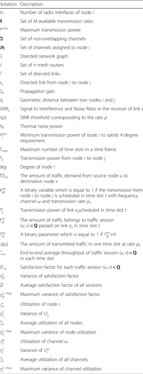
Figure 6 shows that the amount of throughput is
re-duced by about 5 kb/slot, i.e., about 20%, in
HFTTC-TMBF in comparison to the FTTC-TMBF. Due
to the computational complexity reduction in
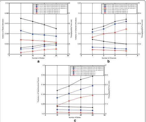
HFTTC-TMBF, this throughput reduction is acceptable. Moreover, Fig. 7a represents the effect of increasing α3 in (41) andα3in (53) on node utilization balancing. It is seen from this figure that by increasing these coeffi-cients, the variance of node utilization and throughput is decreased. Throughput reduction is the result of redu-cing the throughput coefficient in the objective function. Moreover, by increasing the number of nodes, the links length is decreased which is due to the fixed network area. This reduces the interference according to the power control and rate adaptation and therefore, throughput is increased. However, with further increase in the number of nodes, they become closer to each other that increase the interference and therefore, the throughput-increasing slope is decreased. In addition, in-creasing the number of nodes leads to better distribution of traffic among nodes such that it improves the amount of node utilization balancing.


![Fig. 4 The comparison of FTTC-TMBF performance and [9] (a) throughput (b) variance of node utilization (c) variance of channel utilization (d)variance of satisfaction factor](https://thumb-us.123doks.com/thumbv2/123dok_us/912511.1110317/18.595.58.540.86.475/comparison-performance-throughput-utilization-variance-utilization-variance-satisfaction.webp)