Earth Planets Space,56, 893–902, 2004
Three-dimensional inversion for Network-Magnetotelluric data
Weerachai Siripunvaraporn1,2, Makoto Uyeshima2, and Gary Egbert3
1Department of Physics, Faculty of Science, Mahidol University, Rama VI Rd., Rachatawee, Bangkok, 10400, Thailand 2Earthquake Research Institute, University of Tokyo, 1-1-1 Yayoi, Bunkyo-ku, Tokyo 113-0032, Japan
3College of Oceanic and Atmospheric Sciences, Oregon State University, Corvallis, OR 97331, USA (Received May 27, 2004; Revised July 23, 2004; Accepted July 26, 2004)
Three-dimensional inversion of Network-Magnetotelluric (MT) data has been implemented. The program is based on a conventional 3-D MT inversion code (Siripunvarapornet al., 2004), which is a data space variant of the OCCAM approach. In addition to modifications required for computing Network-MT responses and sensitivities, the program makes use of Massage Passing Interface (MPI) software, with allowing computations for each period to be run on separate CPU nodes. Here, we consider inversion of synthetic data generated from simple models consisting of a 1-m conductive block buried at varying depths in a 100-m background. We focus in particular on inversion of long period (320–40,960 seconds) data, because Network-MT data usually have high coherency in these period ranges. Even with only long period data the inversion recovers shallow and deep structures, as long as these are large enough to affect the data significantly. However, resolution of the inversion depends greatly on the geometry of the dipole network, the range of periods used, and the horizontal size of the conductive anomaly.
Key words:Network-Magnetotelluric, data space method, 3-D inversion, Occam’s inversion.
1.
Introduction
The Network-Magnetotelluric (MT) method was first used in central and eastern Hokkaido, in northeastern Japan, in 1989 (Uyeshima et al., 2001). Networks are now widely operated throughout Japan (Uyeshima et al., 2002; Satoh
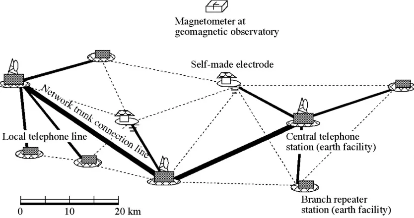
et al., 2001; Yamaguchi et al., 1999), and at some loca-tions in China (Ichikiet al., 2001; Tang et al., 2003a, b). The goal of these observations is to determine the deep and large-scale 3-D electrical conductivity structure of the Earth, and also to monitor electric field variations that may coin-cide with volcanic activities (e.g., at Miyake-jima volcanic island; Sasaiet al., 2002). The method employs a commer-cial telephone network to measure voltage differences over long dipole lengths, ranging from ten to several tens of kilo-meters. Three-component reference magnetic fields are usu-ally obtained from a nearby geomagnetic observatory. A typical Network-MT configuration is shown in Fig. 1. As in conventional MT, Network-MT response functions,Yx(ω)
andYy(ω), can be estimated in the frequency domain using the voltage differenceV(ω)for each dipole and the reference magnetic field,Hrx(ω)andH
Because the electrode spacing between each dipole is quite large, signal-to-noise ratios are generally high. In addition, Network-MT response functions are much less affected by galvanic effects due to small-scale near-surface lateral het-erogeneity of electrical conductivity (Uyeshimaet al., 2001). Network-MT response functions can be related to the con-ventional MT impedance tensor elements, Zx x(ω), Zx y(ω),
Copy right cThe Society of Geomagnetism and Earth, Planetary and Space Sciences (SGEPSS); The Seismological Society of Japan; The Volcanological Society of Japan; The Geodetic Society of Japan; The Japanese Society for Planetary Sciences; TERRA-PUB.
Zyx(ω)andZyy(ω), as described in Uyeshimaet al.(2001).
Forward modeling for both methods is basically identical, except for computation of predicted responses from the mod-eled electric and magnetic fields. Previous efforts to directly interpret Network-MT response data sets have been limited to 2-D and 3-D forward modeling (Uyeshimaet al., 2001, 2002). An indirect interpretation approach is to transform the Network-MT data into conventional MT tensor and then use the available 2-D or 3-D MT inversion schemes to solve for the conductivity distribution (Yamaguchi et al., 1999). The transformation (Uyeshimaet al., 2001) is accomplished by dividing the target region into a set of triangular sections (e.g., as shown by the dashed lines of Fig. 1), and then esti-mating the average impedance tensor at the center of each triangle by fitting the transfer functions for the bounding dipoles. The transformed data itself can be used alone, or together with conventional MT data sets from separate sur-veys (Satohet al., 2001).
Transformation of Network-MT responses into conven-tional MT impedance responses inevitably introduces some errors. For example, for conventional MT the magnetic fields are assumed co-located with the electric fields, while in re-ality for Network-MT, the magnetic fields are obtained from the regional geomagnetic observatory. Thus one implicitly assumes no regional variation in induced magnetic fields.
Here, we describe tests with a 3-D inversion scheme that works directly with the Network-MT response functions, taking account of the actual geometry of the observing sys-tem. The inversion scheme is a straightforward generaliza-tion of the MT inversion scheme described by Siripunvara-porn et al.(2004) and Siripunvaraporn and Egbert (2000). The goal of the inversion is to find the smoothest model sub-ject to an appropriate fit to the data. The inversion algorithm is based on the Occam scheme introduced by Constableet al.
Fig. 1. A sketch of field experiment for Network-MT method (after Uyeshimaet al., 2001). Each dipole is connecting via telephone lines (dashed lines for local lines and thick lines for the Network trunk connection line). The base sites are indicated by the telemetry tower. Usually, magnetic fields are obtained from a geomagnetic observatory in the region.
(1987), but with all computations transformed into the data space. With this data space approach, the size of the system of equations that must be solved is reduced to the number of independent data, N, instead of the number of model pa-rameters,M. With this scheme it is possible to invert modest 3-D MT data sets on a personal computer in a relatively short time (Siripunvarapornet al., 2004). Here, we apply this in-version to synthetic 3-D Network-MT data, to test sensitivity and resolution of these data. In addition, the inversion is cur-rently applied to investigate the 3-D conductivity structure beneath the Hokkaido area and the Miyake-jima volcanic is-land, Japan, and will appear in separated papers.
2.
Data Space Inversion Algorithm
For completeness we briefly summarize the data space inversion algorithm, and then give some details peculiar to inversion of Network-MT data. Further details about the general inversion approach can be found in Siripunvaraporn
et al.(2004) and Siripunvaraporn and Egbert (2000). The goal of the inversion is to find the “smoothest”, or minimum norm, model subject to an appropriate fit to the data. Mathematically this is expressed as:
minimize: (m−m0)TCm−1(m−m0)
subject to: (d−F[m])TCd−1(d−F[m])−X∗2. (2)
In (2),m is the resistivity model,m0 the prior model, Cm the model covariance matrix, d the observed data, F[m] the model response,Cdthe data covariance matrix, and X∗ the desired level of misfit. The Occam approach to this constrained minimization (Constable et al., 1987; see also Parker, 1994) involves linearizing the model responseF[mk]
to find a series of approximate solutions
mk+1(λ)=[λC−m1+
positive semi-definite symmetric matrix. The subscript k
denotes iteration number, andJk=(∂F/∂m)kis theN×M
sensitivity matrix calculated atmk. This approach is a model
space method, since the system of Eqs. (3) is solved in the model space, of dimensionM.
It is not difficult to show that for iterationkthe solution (3) can be expressed as a linear combination of rows of the smoothed sensitivity matrix CmJT (Parker, 1994; Siripun-varapornet al., 2004), i.e.,
mk+1−m0=CmJTkβk+1, (4)
with the coefficient vectorβk+1given by
βk+1=[λCd+JkCmJTk]−
1d¯
k. (5)
This variant of Occam is a data space method, since the sys-tem of Eq. (5) is now solved in the data space, of dimension
N. The main difference between (3) and (5) is that the size of the system of equations to be solved can be dramatically reduced, fromM ×M in the model space, toN×N in the data space. Since in general N will be much less than M, especially for the 3-D MT case, this reorganization of the computations can lead to a great saving on computational costs, both in terms of memory and CPU time.
Whether in the data or model space, a key to the Occam approach (Parker, 1994) is to solve for the updated model
mk+1 for a series of trial values of the damping parameter (or Lagrange multiplier)λ, and compare predictions of the resulting model solution to the data. Initiallyλis adjusted to find the minimum misfit (Phase I). Then, when the misfit has achieved the desired level, λis varied to seek the model of smallest norm with misfit equal the target misfit (Phase II).
2.1 Three-Dimensional Network-MT Forward Model-ing
W. SIRIPUNVARAPORNet al.: THREE-DIMENSIONAL INVERSION FOR NETWORK-MAGNETOTELLURIC DATA 895
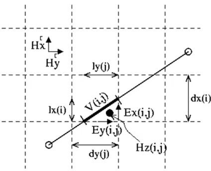
Fig. 2. Sketch showing how to compute Network-MT responses from a staggered-grid numerical solution for electric fields. In this figure, the voltageV(i,j), is computed as a sum over electric components defined on cell edges and vertical magnetic fields. Notation: dx(i)anddy(j) are grid cell dimensions, whilelx(i)andly(j) are distance projected from sub-dipole (thick line) onto thex- andy-directions.ExandEyare electric fields inx- andy-directions on the cell edge andHzis the vertical magnetic field. Hr
xandHyrare horizontal magnetic field components at the remote observatory.
Maxwell’s equation, defined in terms of the electric fields, with a staggered grid finite difference approximation (Smith, 1996; Siripunvarapornet al., 2002). This scheme has proven to be accurate and robust.
In order to obtain Network-MT responses, Yx(ω) and
Yy(ω), from (1), we must compute voltage differencesV(ω)
between the ends of the dipoles, i.e., the integral of electric fields along the dipole lines at the surface. Together with the magnetic fields computed at the actual observatory lo-cation, we can then obtain the predicted Network-MT re-sponses for any given model solutions. Computation of the required dipole line integrals is outlined in Fig. 2. First, the Network-MT dipole line is subdivided into many seg-ments, where each segment lies within a single grid cell (de-noted by the dashed lines in Fig. 2). The voltage difference along each dipole segment (the thicker line in Fig. 2) can be estimated using the horizontal electric fieldsEx(i,j)and
Ey(i,j)defined on the edges of the staggered grid cells, and the vertical magnetic field Hz(i,j) computed in the usual way from the electric field solution. According to Faraday’s law, the induced EMF around the closed triangular loop is
Vz(i,j)= 12iωμHz(i,j)lxly. Hence, the voltage difference
V(i,j)along the diagonal segment can be estimated as:
V(i,j)=Vx(i,j)+Vy(i,j)−Vz(i,j)
=Ex(i,j)lx+Ey(i,j)ly−
1
2iωμHz(i,j)lxly. (6)
The total voltage difference can then be computed as the sum of the voltage differencesV(i,j)of all segments along the full dipole.
For forward computations the problem must be solved for external magnetic sources in both the x and y direc-tions (x-polarization or y-polarization). Each polarization results in magnetic field vectors, (Hr
x,x−pol,H
also voltage differences, Vx−pol andVy−pol. The
Network-MT response (Yx,Yy) of each frequency in (1) can then be
and then directly compared to the observed Network-MT responses to invert for conductivity (Uyeshimaet al., 2001).
2.2 Sensitivity Matrix for Network-MT responses
To compute the gradient of the model responses with re-spect to the model,Jk=(∂F/∂m), we use the reciprocity
ap-proach described in Rodi (1976), which we summarize here. From (7) the responses are Y = [YxYy]T = H−1V. To simplify the sensitivity calculations, we assume that the mag-netic fields are only weakly affected by changes in the model relatively to the perturbation of electric fields. Note that we only make this approximation for sensitivity calculations, not for comparison of predicted and observed data. This small approximation should not cause any problems for the convergence of the inversion. Many studies have confirmed that approximate sensitivities can be effectively used in the inversion (Smith and Booker, 1988; Farquharson and Old-enburg, 1996; Siripunvaraporn and Egbert, 2000). This ap-proximation leads to∂Y/∂m=H−1∂V/∂m. From (6),Vin turn can be written as a linear function of the electric fields
edefined on the staggered grid, i.e.,V=gTe, whereg con-tains all coefficients used to estimate Vas outlined above. Sincegdoes not depend uponm
∂V/∂m=gT∂e/∂m. (8)
With the staggered grid finite difference approximation,eis obtained by solving the system of equationAe =b, where
A is the coefficient matrix of the second order Maxwell equations, andbdefines boundary conditions. Perturbations to the model parameters δm result in perturbations to the coefficient matrix, and to the electric field solution satisfying (A+δA)(e+δe) = b. Using Ae = b and dropping second order terms we thus have δe = −A−1δAe. It is straightforward to write the vectorδAe =Eδm, where the matrixEdepends on the unperturbed electric field solution
e, and the details of the model parameterization. Thus we have for the perturbation to the computed potentials: δV =
−gTA−1Eδm, so that
∂V/∂m= −gTA−1E. (9)
Rather than compute the derivative terms in (9) by solving
Mforward problems, the reciprocity approach computes the derivatives as
∂V/∂mT =ET(AT)−1g=ETA−1g. (10)
The last equality holds because for the frequency domain Maxwell’s equations, the coefficient matrix can be scaled to be symmetric. Calculation of sensitivities for all data can thus be reduced to solvingNd(=number of dipoles) forward problems, rather than theMforward problems suggested by a direct implementation of (9)
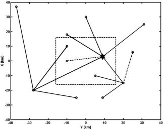
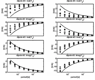
Fig. 3. Dipole configuration used to generate synthetic data sets used to test the inversion code. The data were generated for 12 dipole lines from 3 base sites. The site for the magnetic field is located at the base site marked with the star. The dashed line indicates the boundary of the buried 1-m conductor buried. Network-MT responses for the dipoles denoted by the dashed line (dipole #3) and dash-dot line (dipole #11) are shown in Fig. 9.
the iterative solver is terminated when the normalized resid-ual reaches 10−4, instead of 10−8 as is used when comput-ing responses for comparison with data. Siripunvaraporn
et al. (2004) show that this early termination strategy re-duces computational time by more than 70 percent, with-out affecting inversion results. Curiously, however we have found that Network-MT sensitivity calculations require sig-nificantly more iterations than MT sensitivities to achieve the same level of misfit. The program therefore requires a lot more computational time than for the conventional MT case. The reason for this slower convergence is not com-pletely clear, but this may result from the more complicated form for the vectorg, with many more non-zero components than in the MT case.
Other parts of the inversion, such as implementation of the model covariance and the optimization algorithm are ba-sically the same as in Siripunvarapornet al.(2004).
2.3 Computational Details: MPI Implementation
All inversions are performed on SGI LX3700 parallel computers with MPI (Massage Passing Interface) implemen-tation. With MPI, the forward modeling and the sensitivity calculation for each period are assigned to run separately on each CPU node. The results are then combined to solve (5) on one CPU node. In theory, the CPU time per iteration is equal to the computational time of just one period, plus some overhead time when solving (5).
3.
Synthetic Data Examples and Discussions
To test the algorithm and explore the sensitivity and reso-lution of network MT data, we ran the inversion program on a series of synthetic data sets generated from simple models of buried conductive prisms. The model consists of a 1-m conductive block with a dimension of 32 km×32 km×10km in a 100 -m homogeneous background (Fig. 3). The conductor is buried at three different depths: 6, 10 and 20 km, referred to respectively as cases I, II and III. The basic dipole configuration used for initial tests is shown on top of Fig. 3. These 12 dipoles mimic data collected in field ex-periments (Uyeshimaet al., 2001). There are 3 main base stations, with a single magnetic station located at the base station near the middle (shown as a star in Fig. 3). In general, Network-MT data have been collected at low sampling rates, typically 1 Hz or less. However, in practice, real field data sets often exhibit high coherency for periods between 300 and 40,000 seconds, with significantly reduced coherency at shorter (and longer) periods, due primarily to cultural noise and other factors, such as telephone line noise. To maintain relevance to real Network-MT field data, we thus generated synthetic data at 8 periods, evenly spaced on a logarithmic scale from 320 to 40,960 seconds for our base case. To ex-plore the value of higher frequency data, some tests were also done with additional periods, between 3 and 100 sec-onds. The synthetic responses were then contaminated with Gaussian noise, with variance 5% of|YxYy|12. The total
num-ber of data for our base case isN =384 (4 real responses for each of 12 dipoles at 8 periods). The model mesh used for the inversion is 36×36×31 (plus 7 air layers) resulting in
M =40,176 model parameters. All inversions were started from a 30-m half space.
in-W. SIRIPUNVARAPORNet al.: THREE-DIMENSIONAL INVERSION FOR NETWORK-MAGNETOTELLURIC DATA 897
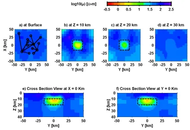
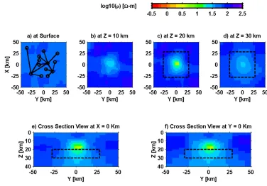
Fig. 4. Inverted model for synthetic data case I obtained with only 8 long periods. The conductor is buried at 6 km depth. Dashed lines indicate the boundary of the conductor. Panels a)–d) are horizontal slices at the 0, 10, 20 and 30 km depth, respectively. Panels e) and f) are cross section atX= 0 km, andY= 0 km, respectively.
Fig. 5. Inverted model for synthetic case I (conductor buried at 6 km depth), obtained using both short and long period data. Inverse solution sections are as in Fig. 4.
dicating the outline of the buried conductor. In this case, the inversion has no trouble in retrieving the conductor buried at 6 km depth. However, the conductivity contrast, lateral ex-tent, and depth of the conductor are not completely accurate. Including the additional 4 shorter period data (3–100 sec-onds) improves the result, with the conductivity contrast and depth now quite reasonable (Fig. 5). However, the conduc-tive anomaly in the inverse solution is still somewhat reduced in size.
struc-Fig. 6. Inverted model for synthetic case II (10 km deep conductor) with only 8 long periods. Inverse solution sections are as in struc-Fig. 4.
Fig. 7. Inverted model for synthetic case II (10 km deep conductor) with both short and long periods. Inverse solution sections are as in Fig. 4.
ture can be improved by addition of shorter period data. But many other factors must also be taken into account, includ-ing data noise levels, the configuration of dipoles, and the nature of the shallow anomaly itself.
As for case I, in both cases II and III the inversion requires only about 4–5 iterations for both Phases I and II. The result-ing inverse solutions are shown in Figs. 6 and 8 for cases II and III, respectively. Although in both cases the calculated responses fit the observed responses to within a RMS mis-fit of 1 (i.e., within 5% relative error), the inverse solution
W. SIRIPUNVARAPORNet al.: THREE-DIMENSIONAL INVERSION FOR NETWORK-MAGNETOTELLURIC DATA 899
Fig. 8. Inverted model for synthetic case III (20 km deep conductor) with only 8 long periods. Inverse solution sections are as in Fig. 4.
Fig. 9. Network-MT responses,YxandYy, both real and imaginary parts for dipole #3 (dashed line in Fig. 3) and dipole #11 (dash-dot line in Fig. 3). Stars are for case I, squares for case II, diamonds for case III, and solid lines give the response of a 100-m half-space. Crosses are for the deeply (20 km) buried conductor similar to case III, but with the root extended to 80 km depth. Circles are for a conductor buried at 20 km depth, but horizontally extended to cover a larger area. For clarity, no noise is added to this figure.
of the inversion (not shown) remains essentially as in Fig. 8. As case I demonstrates, long period data can be used to probe shallow structure, if the anomaly is presented in the data. However, if the conductor is buried more deeply, as in case III, the inversion does not recover the correct structure, but instead finds a simpler model that still fits the data at the target level. The failure in recovering the conductor
does not imply a failure of the inversion scheme, but rather reflects the fact that the Network-MT responses for the array configuration shown in Fig. 3 are only minimally affected by this deep conductor. Figure 9 shows selected network-MT responses for cases I-III. For case III (diamonds) bothYx
andYy deviate very little from the response of a 100-m
Fig. 10. Inverted model for synthetic case III, with the dipole configuration shown in a), obtained using only 8 long periods. The conductor is buried at 20 km. Inverse solution sections are as in Fig. 4.
Fig. 11. Inverted model using only 8 long periods. In this case, the conductor is buried at 20 km depth, but its size is increased horizontally to 56 km× 56 km. Labels are the same as in Fig. 4.
for shallower burial of the conductor as in cases I (stars) and II (squares). Because responses for a deep conductor differ little from those of a homogeneous model, the inversion can fit the data by making the middle part of the model slightly less resistive than the surrounding area.
One way to increase the sensitivity of the data to the con-ductor and thus improve resolution is to increase the number of dipoles to cover a larger area. We test the effect of this modification for the deep conductor of Case III, using an
W. SIRIPUNVARAPORNet al.: THREE-DIMENSIONAL INVERSION FOR NETWORK-MAGNETOTELLURIC DATA 901
data to the inversion may improve this situation somewhat. As the above experiment shows, resolution of model fea-tures may depend to some extent on the number and con-figuration of dipoles. The geometry of the target anomalies also plays a role. Two additional tests demonstrate that the dipole configuration of Fig. 3 can still be sensitive to a deep (20 km) conductor, if the anomaly is larger in size. For both cases we used only the 8 long periods, comparable to the real field data. Again 5% Gaussian noise was added to the syn-thetic responses before inversion. In both cases, the conduc-tor is buried at 20 km depth. First, we expand the thickness of the conductor from 10 km to 60 km, while keeping hori-zontal dimensions the same. The inversion again converges in 4 iterations to fit the data within a RMS misfit of 1. The resulting conductivity model is essentially the same as that shown in Fig. 8, with no evidence of the conductor. This is not surprising, since extending the root of the conductor deeper has little effect on the data. The Netwpork-MT re-sponses (crosses in Fig. 9) are almost identical to those for the standard array configuration for case III (diamonds).
As a second test, the 20 km deep conductor is expanded horizontally to 56 km×56 km, while keeping the same 10 km thickness. The inverted model is shown in Fig. 11 af-ter 5 iaf-terations required to reduce the RMS misfit to 1. Ex-tending the conductor horizontally increases the sensitivity of the data to deep conductive structure, as shown by the cir-cles in Fig. 9. However the effect is still less significant than in the case where the conductor is shallow. Similar to other cases, the depth and size of the conductor were still not well-estimated. Resolution of depth can be improved if shorter periods are included, but the horizontal scale of the conduc-tor is still underestimated as in Figs. 5 and 7.
4.
Conclusions
We have developed a 3-D inversion for Network-MT data, based on the data space Occam’s inversion for conventional MT data of Siripunvarapornet al.(2004). With the imple-mentation of MPI, computations for many periods can be done simultaneously, leading to significantly reduced run times. By running forward modeling and sensitivity calcula-tions for one period on one CPU, the total run time is compa-rable to that required for just one period, plus some overhead for solving Eq. (5).
As discussed by Uyeshimaet al.(2001), one important ad-vantage of the Network-MT method is that short scale near surface galvanic distortion in the data is reduced with long dipole lines. In addition, the quality of long period data can be much better than what is obtained from conventional MT, since the longer dipole line significantly reduce the effects of electrode noise. However, telephone line noise may re-duce data quality at shorter periods, and the lack of short period data may limit the ability of the inversion to constrain anomaly depth.
Our results show that the long period data by itself can be used to recover the anomaly whether it is shallow or deep, if it is adequately presented in the data. The sensitivity of the data to an anomaly will depend on the number and configuration of dipoles, which must be considered carefully in assessing whether a feature could in principal be resolved. One consistent feature in the examples above is that the
lateral extent of the conductor in the inverted model is always smaller than it should be. This can be explained by the sampling characteristics of the Network-MT method. Near the boundary of a conductor or resistor, electric fields are high on one side and low on the other. The Network-MT response of a dipole that crosses the anomaly boundary is essentially an average of the electric fields over both sides of the anomaly, resulting in loss of information about the location of the sharp horizontal boundary. This makes it difficult for the inversion to properly locate the edge of the buried conductive feature in these synthetic data examples.
Particularly if short period data is not available, the ability of Network MT to correctly image both depths and lateral boundaries of conductive features may be limited. In many cases higher quality short period data may be obtained with a conventional MT approach. This data would also allow better resolution of lateral boundaries of shallow conductive features. The methods described here can be easily extended to allow joint inversion of both data types, which may well provide the best resolution of both shallow and deep struc-tures. Another possibility is to run the inversion with prior information inm0. This will help improve the lateral and ver-tical resolution of the inverted model. This prior information can come from other geophysical studies, such as gravity or seismic methods, in real field data set.
Acknowledgments. This research has been supported a JSPS post-doctoral fellowships (P02053) and a grant from MEXT, Japan (02053) to W. S. and M. U, and by DOE-FG0302ER15318 to G. E., and partially supported by a grant from the Thailand Research Fund (TRF:PDF/37/2543) to W. S. The authors would like to thank Colin Farquharson and an anonymous reviewer for their comments to help improving the manuscript.
References
Constable, C. S., R. L. Parker, and C. G. Constable, Occam’s inversion: A practical algorithm for generating smooth models from electromagnetic sounding data,Geophys.,52, 289–300, 1987.
Farquharson, C. G. and D. W. Oldenburg, Approximate sensitivities for the electromagnetic inverse problem,Geophys. J. Inter.,126, 235–252, 1996. Ichiki, M., M. Uyeshima, H. Utada, G. Zhao, J. Tang, and M. Ma, Upper mantle conductivity structure of the back-arc region beneath northeastern China,Geophys. Res. Lett.,28, 3773–3776, 2001.
Parker, R. L.,Geophysical Inverse Theory,Princeton Univ. Press., 1994. Rodi, W. L., A technique for improving the accuracy of finite element
solutions for Magnetotelluric data,Geophys. J. Roy. Astr. Soc.,44, 483– 506, 1976.
Sasai, Y., M. Uyeshima, J. Zlotnicki, H. Utada, T. Kagiyama, T. Hashimoto, and Y. Takahashi, Magnetic and electric field observations during the 2000 activity of Miyake-jima volcano, Central Japan,Earth Planet. Sci. Lett.,203, 769–777, 2002.
Satoh, H., Y. Nishida, Y. Ogawa, M. Takada, and M. Uyeshima, Crust and upper mantle resistivity structure in the southeastern end of the Kuril Arc as revealed by the joint analysis of conventional MT and network MT data,Earth Planets Space,53, 829–842, 2001.
Siripunvaraporn, W. and G. Egbert, An efficient data-subspace inversion method for 2-D magnetotelluric data,Geophys.,65, 791–803, 2000. Siripunvaraporn, W., G. Egbert, and Y. Lenbury, Numerical accuracy of
magnetotelluric modeling: A comparison of finite difference approxima-tions,Earth Planets Space,54, 721–725, 2002.
Siripunvaraporn, W., G. Egbert, Y. Lenbury, and M. Uyeshima, Three-dimensional magnetotelluric inversion: Data space method,Phys. Earth Planet. Inter., 2004 (in press).
Smith, J. T., Conservative modeling of 3-D electromagnetic fields, Part II: Biconjugate gradient solution and an accelerator,Geophys.,61, 1319– 1324, 1996.
struc-ture,Geophysics,53, 1565–1576, 1988.
Tang, J., M. Uyeshima, H. Utada, G. Zhao, M. Ichiki, M. Ma, and Y. Liu, Preliminary results of long period MT and GDS in Liaoning Province, NE China, Proc. Conductivity Anomaly Meeting 2003, 66–73, 2003a. Tang, J., H. Utada, G. Zhao, M. Uyeshima, Y. Liu, X. Jiang, M. Ichiki, and
M. Ma, The Mantle Conductivity Structure Beneath Jilin And Liaoning Province, NE China,Annual of the Chinese Geophysics Society,575–576, 2003b.
Uyeshima, M., H. Utada, and Y. Nishida, Network-magnetotelluric method and its first results in central and eastern Hokkaido, NE Japan,Geophys. J. Int.,146, 1–19, 2001.
Uyeshima, M., M. Ichiki, I. Fujii, H. Utada, Y. Nishida, H. Satoh, M. Mishina, T. Nishitani, S. Yamaguchi, I. Shiozaki, H. Murakami, and N.
Oshiman, Network-MT survey in Japan to determine nation-wide deep electrical conductivity structure, inSeismotectonics in Convergent Plate Boundary,edited by Y. Fujinawa and A. Yoshida, pp. 107–121, Terrapub, 2002.
Yamaguchi, S., Y. Kobayashi, N. Oshiman, K. Tanimoto, H. Murakami, I. Shiozaki, M. Uyeshima, H. Utada, and N. Sumitomo, Preliminary report on regional resistivity variation inferred from the Network MT investigation in the Shikoku district, southwestern Japan,Earth Planets Space,51, 193–203, 1999.