R E S E A R C H
Open Access
Hyperspectral image classification with SVM
and guided filter
Yanhui Guo
1, Xijie Yin
1*, Xuechen Zhao
1, Dongxin Yang
2and Yu Bai
3*Abstract
Hyperspectral image (HSI) classification has been long envisioned in the remote sensing community. Many methods have been proposed for HSI classification. Among them, the method of fusing spatial features has been widely used and achieved good performance. Aiming at the problem of spatial feature extraction in spectral-spatial HSI classification, we proposed a guided filter-based method. We attempted two fusion methods for spectral and spatial features. In order to optimize the classification results, we also adopted a guided filter to obtain better results. We apply the support vector machine (SVM) to classify the HSI. Experiments show that our proposed methods can obtain very competitive results than compared methods on all the three popular datasets. More importantly, our methods are fast and easy to implement.
Keywords:Support vector machine, Guided filter, Hyperspectral image classification
1 Introduction
Hyperspectral imaging sensors have been widely used in
remote sensing, biology, chemometrics, and so on [1].
Hyperspectral imaging sensors can obtain spatial and spectral information of materials, which is called the hyperspectral image (HSI), for the same time. Due to abundant spectral information, HSI is widely applied to material recognition and classification, such as land cover [2], environmental protection [3], and agriculture [4]. Hence, HSI classification has attracted increasing atten-tion and became a hot topic in the remote sensing community.
The task of classification is to assign a unique label to each pixel vector of HSI. For this problem, many pixel-wise (spectral-based) methods were employed,
in-cluding k-nearest neighbors (KNN) [5], support vector
machine (SVM) [6], and sparse representation [7] in the last two decades. SVM has shown good performance for classifying high-dimensional data when a limited
number of training samples are available [8]. It can
effectively overcome the Hughes phenomenon [9] and
the problem of limited training samples in HSI classi-fication. Therefore, SVM and its improved algorithms
get better performance than other methods. However, they still have a wide gap for expectations. After all, it is a universal phenomenon that different materials have the same spectrum and the same material has different spectrum.
To overcome the above problem and improve the per-formance of classification, recent studies have suggested incorporating spatial information into a spectral-based classifier [10], which is called the spectral-spatial HSI classification. Because of the continuous improvement in spatial resolution, the spatial features of materials be-come more representative. Many papers show that spec-tral method is a very effective way for HSI classification. Various types of classification approaches have been
pro-posed, including morphology feature extraction [11],
kernel combination [3,12], and joint representation [13]. By using geodesic opening and closing operations with fixed shape structuring elements of different sizes, mor-phological profiles significantly improve the classification accuracy. The main idea of a joint representation model is to exploit both spectral and spatial features by treating the test sample as a collection of its neighboring pixels (including the test pixel itself ).
For SVM methods, the mainstream approaches of fusing spectral and spatial features are used by kernel combin-ation [14]. The paper [15] proposed a series of composite kernels to fuse spectral and spatial features directly in the
* Correspondence:[email protected];[email protected] 1Shandong Women’s University, Ji’nan 250300, Shandong, China 3California State University, Fullerton, CA 90831, USA
Full list of author information is available at the end of the article
to extract spatial features. Compared to the reference
[18], our contribution can be concluded as extracting
spatial features before classification. In more detail, the main contributions are listed as follows.
1) We adopt the guided filter to smooth HSI, which is similar to de-noising in image processing. By this method, a fusion which consists of a pixel and its neighboring pixel information is generated. It is proved to be simple and effective.
2) We attempt different spectral and spatial fusion methods, which makes sense for future work. 3) The proposed methods are applied to three widely
used hyperspectral datasets. We compare with two methods by three evaluation metrics.
2 Related methodology and work
2.1 SVM and HSI classification
SVM is a supervised machine learning method, proposed by Vapnik [19], which is based on the statistical learning theory. Essentially, SVM attempts to find a hyperplane in the multidimensional feature space to separate the two classes. And this hyperplane is the best decision surface which maximizes the distance between the hyperplane and two classes, called the margin. Generally, the larger the margin, the better the classifier is. From a given set of the training set, obtaining an SVM model is equivalent to an optimization problem for finding a hyperplane. For this optimization, SVM introduces a structural minimum principle that prevents over-fitting problems.
SVM is suitable for high-dimensional data with the limited training set. And a lot of researches have ad-dressed that SVM classifier presents superior per-formance on HSI classification [6, 20], compared with
other popular classifiers such as decision tree
classifier, k-nearest neighbor classifier, and neural net-works. The power of SVM is mainly due to its kernel function, especially radial basis function. However, the single kernel is not enough for all cases. Some
re-searchers proposed a composite kernel [21], which
in-tegrates both spectral and spatial features, to improve classification performance.
where ak and bk are a linear coefficient and bias, re-spectively. From the model, we can see that ∇q=a∇g, which means that the outputqwill have a similar
gradi-ent with guidance image g. The coefficient and bias,
which need to be known, are solved by a minimum cost function as follows:
Here,ϵis a regularization parameter. According to the paper [22], a solution can be derived from Eq. (2) as
pinωk. After obtaining the coefficient akand bk, we can
compute the filtering output qi. Through the above
process, we can get a linear transform imageq.
The guided filter was first used for HSI classifica-tion by Kang [18]. They considered the HSI classifica-tion as a probability optimizaclassifica-tion process. They firstly obtained the initial probability by SVM. Then, they applied a guided filter to optimize the initial probabil-ity maps. They got a state-of-the-art result.
Subse-quently, Wang [23] adopted a guided filter to extract
the spatial features from HSI. Then, a stacked
autoen-coder was used to classify each pixel. Guo [24]
3 HSI classification with SVM and guided filter
3.1 The proposed Guided Filter SVM Edge Preserving Filter (GF-SVM-EPF)
We propose a novel method for HSI classification with SVM and guided filter. First, we extract the spatial features of HSI by the guided filter, which is obtained from the original HSI by a principal compo-nent analysis (PCA) method. Then, we classify the spatial features by SVM. Finally, we employ a guided filter again to optimize the classification. The process is shown in Fig. 1.
3.1.1 Extracting spatial features by guided filter
First, we obtain a guidance image by PCA. We take the first three principal components as a color guidance image. Given a datasetD= {d1,d2,⋯,dS}, we adopt PCA to obtain the following result. Herediis the information of theith band, and S denotes the number of bands.
g1;g2;⋯;gS
½ ¼PCAð ÞD ð5Þ
So, the guidance image isG= [g1,g2,g3].Then, based on formula (1), using input imaged1and guidance imageG,
Fig. 1Framework of HSI classification by the proposed method. Original HSI was used to get the guidance image (filter) and decomposed HSI by
PCA firstly. Then, decomposed HSI was filtered by a guidance filter. Subsequently, a SVM classifier was adopted to get the classification map. Finally, edge preserving filter was applied to optimize the classification map
3.2 Other methods
In order to verify the effectiveness of our method, we also proposed another three methods with SVM and guided filter. We want to research the efficacy of spatial feature extraction and propose a GF-SVM method, which firstly extracts spatial features and then classifies them by SVM. The implementation is the same as the steps 1 and 2 in Section3.1.
If spatial features and spectral features are fused to-gether, can the increasement of information improve classification accuracy of the HSI? We proposed another method called Co-SVM (Connected SVM). We choose the top half of [g1,g2,⋯,gS] as the original feature. And we choose the top half ofUas the spatial features. Then we join the original and the spatial features together as a fusion feature to classify. After being classified by SVM, we get the final classification. By optimizing the result of
Co-SVM as step 3 in Section3.1, we got another method
called Co-SVM-EPF.
4 Results and discussion
4.1 Experimental setup 4.1.1 Datasets
Three hyperspectral data,2 including Indian Pines, Uni-versity of Pavia, and Salinas, are employed to draw a convincing conclusion. The Indian Pines dataset was gathered by an AVIRIS sensor. The image scene, with a spatial coverage of 145 × 145 pixels, is covering the
woods, grass-pasture, and so on. We choose 200 spectral channels from 220 bands in the 0.4- to 2.45-μm region of the visible and infrared spectrum.
The University of Pavia dataset was captured by the ROSIS (Reflective Optics System Imaging Spectrometer) sensor. The dataset contains 610 × 340 pixels with 115 spectral bands. After removing water absorption and low SNR bands, 103 bands were used for the analysis. And there are nine categories to be classified.
The third dataset was collected by the AVIRIS sensor, capturing an area over Salinas Valley, California, with a high spatial resolution of 3.7 m. Salinas comprises 512 × 217 pixels in all and contains vegetables, bare soils, and vineyard fields. We also selected 200 bands for experi-ments by discarding 20 water absorption.
4.1.2 Evaluation metrics
Three widely used indexes for HSI classification were adopted to evaluate the performance of experimental methods, including the overall accuracy (OA), the aver-age accuracy (AA), and the kappa coefficient (KA).
4.1.3 Parameter settings
In this experiment, we use libSVM designed by Lin [25].
The libSVM has two main parametersCandgto be set.
The Cand g are determined by cross validation. AndC
changes from 10−2to 104, andgranges from 2−1to 24.
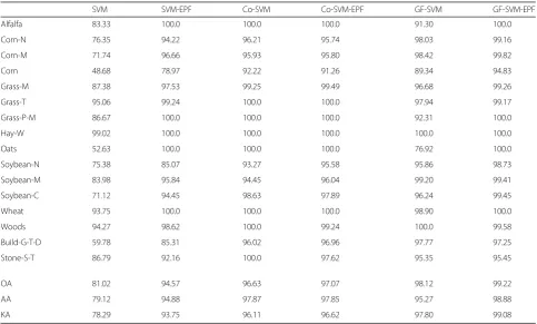
Table 1Classification accuracy on the Indian Pines dataset (10% samples for training)
SVM SVM-EPF Co-SVM Co-SVM-EPF GF-SVM GF-SVM-EPF
Alfalfa 83.33 100.0 100.0 100.0 91.30 100.0
Corn-N 76.35 94.22 96.21 95.74 98.03 99.16
Corn-M 71.74 96.66 95.93 95.80 98.42 99.82
Corn 48.68 78.97 92.22 91.26 89.34 94.83
Grass-M 87.38 97.53 99.25 99.49 96.68 99.26
Grass-T 95.06 99.24 100.0 100.0 97.94 99.17
Grass-P-M 86.67 100.0 100.0 100.0 92.31 100.0
Hay-W 99.02 100.0 100.0 100.0 100.0 100.0
Oats 52.63 100.0 100.0 100.0 76.92 100.0
Soybean-N 75.38 85.07 93.27 95.58 95.86 98.73
Soybean-M 83.98 95.84 94.45 96.04 99.20 99.41
Soybean-C 71.12 94.45 98.63 97.89 96.24 99.45
Wheat 93.75 100.0 100.0 100.0 98.90 100.0
Woods 94.27 98.62 100.0 99.24 100.0 99.58
Build-G-T-D 59.78 85.31 96.02 96.96 97.77 97.25
Stone-S-T 86.79 92.16 100.0 97.62 95.35 95.45
OA 81.02 94.57 96.63 97.07 98.12 99.22
AA 79.12 94.88 97.87 97.85 95.27 98.88
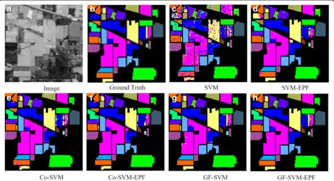
4.2.1 Experimental results and discussion on Indian Pines
The Indian Pines dataset is the most commonly used and the most difficult to classify. In this experiment, the classification accuracy for each class, OA, AA, and KA is adopted to evaluate the classification performance.
Figure 2 shows the classification maps obtained by
dif-ferent methods associated with the corresponding OA scores. From this figure, we can see that the classifica-tion accuracy obtained by SVM is the worst since lots of noisy estimations are visible. The best one is the classifi-cation accuracy obtained by GF-SVM-EPF, which is al-most the same as the ground truth.
Classification performance of each class is shown in
Table1. All our proposed methods outperform the SVM
and EPF significantly on all the indexes. They are higher than EPF by 2%, 2.5%, 3.5%, and 4.6%, respectively. Espe-cially, the proposed method GF-SVM-EPF achieves 99.22%, which is the best result we have seen so far. In 16 categories, there are 11 classes to reach the highest results. Unlike our expectations, the result obtained by Co-SVM which employs the fusion of guided informa-tion and spectral informainforma-tion is worse than that ob-tained by GF-SVM which only employs the guided
of Pavia dataset
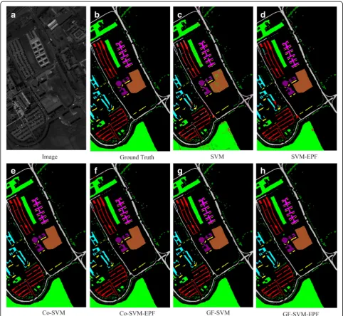
The University of Pavia only has nine categories. It is easier to classify. Classification maps of different methods are illustrated in Fig.3. It can be seen from this figure that the proposed methods (Co-SVM, GF-SVM, and GF-SVM-EPF) achieve better classification perform-ance than other compared approaches. Especially, in the map of GF-SVM-EPF, we can hardly see the difference between it and the ground truth.
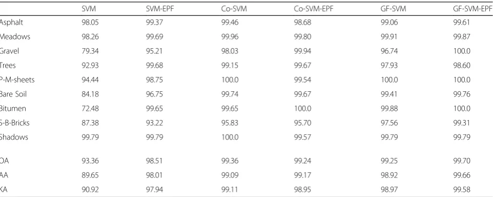
And the results of different methods are shown in
Table 2. It can be seen from Table 2 that our proposed
methods (Co-SVM, Co-SVM-EPF, GF-SVM) are similar, and they are slightly higher than SVM-EPF (98.51%). GF-SVM-EPF obtains the result of 99.7%, which outper-forms state-of-the-art methods. There are six categories to reach the highest results in nine categories. In this ex-periment, there is a strange phenomenon that Co-SVM is better than Co-SVM-EPF. That is because some pixels of the thin edges are divided into the background, as
seen from Fig. 3. As in the previous experiment, the
method of extracting spatial features by the guided filter twice (GF-SVM-EPF) is the most effective classification method.
Table 2Classification accuracy on the University of Pavia dataset (10% samples for training)
SVM SVM-EPF Co-SVM Co-SVM-EPF GF-SVM GF-SVM-EPF
Asphalt 98.05 99.37 99.46 98.68 99.06 99.61
Meadows 98.26 99.69 99.96 99.80 99.91 99.87
Gravel 79.34 95.21 98.03 99.94 96.74 100.0
Trees 92.93 99.68 99.15 99.67 97.93 98.60
P-M-sheets 94.44 98.75 100.0 99.54 100.0 100.0
Bare Soil 84.18 96.75 99.74 99.67 99.41 99.76
Bitumen 72.48 99.65 99.65 100.0 99.88 100.0
S-B-Bricks 87.38 93.22 95.83 95.70 97.56 99.31
Shadows 99.79 99.79 100.0 99.57 99.79 99.79
OA 93.36 98.51 99.36 99.24 99.25 99.70
AA 89.65 98.01 99.09 99.17 98.92 99.66
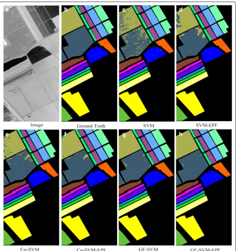
4.2.3 Experimental results and discussion of the Salinas dataset
The last experiment is performed on the Salinas dataset, which is the biggest one we have chosen. The qualitative results are shown in Fig.4. It is apparent from this figure that the map of GF-SVM-EPF has the fewest noise points and obtains the best results.
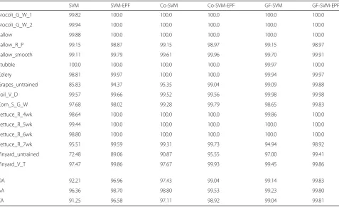
The detailed results are illustrated in Table 3. All the methods perform well on this dataset. The worst is about 92.21% by SVM. The proposed methods (Co-SV-M-EPF, GF-SVM, and GF-SVM-EPF) are all over 99%, especially GF-SVM-EPF which reaches 99.8%, outper-forming other methods greatly. There are 12 categories to achieve the best result in 16 categories. The
conclusion of this experiment is consistent with that of Indian Pines. Spectral features with spatial features can improve classification accuracy. The result of extracting spatial features twice is better than that of extracting spatial features once.
From the above three experiments, we can draw a conclusion that SVM with guided filter can be well used for HSI classification. The guided filter is an effective way to fuse spatial information and spectral information. Especially for datasets with a regular shape, a guided fil-ter is more effective to extract spatial features. Because the filtered pixels contain not only neighbor information but also their own information, they can be directly used for classification without adding other information.
5 Conclusion
In this paper, we propose several spectral-spatial HSI classification methods which combined SVM with guided filter. Two spectral and spatial fusion methods are adopted for the SVM. Moreover, the guided filter was used for extracting spatial information and optimiz-ing the classification results, respectively. Our proposed methods can improve the classification accuracy signifi-cantly in a short time. Consequently, the proposed methods can be effective to real applications.
From this work, we can draw the following conclusions: (a) The guided filter is an effective way to extract spatial in-formation in HSI. (b) The extracted feature by the guided
filter is good enough for HSI classification, without original information. (c) The method of SVM with twice filtrations is a simple and effective way to classify HSI.
6 Endnotes
AA:Average Accuracy; Co-SVM: Connected SVM; GF-SVM-EPF: Guided Filter SVM Edge Preserving Filter; HSI: Hyperspectral Image; KA: Kappa Coefficient; KNN: k-nearest neighbors; OA: Overall Accuracy; PCA: Principal Component Analysis; ROSIS: Reflective Optics System Imaging Spectrometer; SVM: Support Vector Machine
Funding
The project was supported by Open Research Fund of Shandong Provincial Key Laboratory Of Infectious Disease Control and Prevention, Shandong Center for Disease Control and Prevention (No.
2017KEYLAB01), the Science and Technology Project for the Universities of Shandong Province (No. J18KB171), Laboratory of Data Analysis and Prediction in Shandong Women’s University.
Availability of data and materials
The simulations were performed using matlab2014a and libsvm3.0 in Intel Core I7 (64bit). All data generated or analyzed during this study are included in this published article. The hyperspectral image datasets can be
downloaded athttp://www.ehu.eus/ccwintco/ index.php?title=Hyperspectral_Remote_Sensing_Scenes
Authors’contributions
YHG is the main writer of this paper. He proposed the main idea and designed the experiment. XJY and XCZ completed the analysis of the results.
Corn_S_G_W 97.68 98.02 99.28 99.79 98.65 99.83
Lettuce_R_4wk 98.64 100.0 100.0 100.0 99.86 100.0
Lettuce_R_5wk 99.44 100.0 100.0 100.0 100.0 100.0
Lettuce_R_6wk 98.80 100.0 100.0 100.0 100.0 100.0
Lettuce_R_7wk 95.51 99.59 99.31 99.73 94.94 98.92
Vinyard_untrained 72.48 89.06 90.87 95.55 97.00 99.41
Vinyard_V_T 97.47 99.86 97.67 99.93 99.45 99.86
OA 92.21 96.96 97.43 99.04 99.14 99.83
AA 96.36 98.70 98.80 99.53 99.23 99.80
DXY assisted in the collection and pre-processing of the data. YB refined the idea and designed the structure of the whole manuscript. Both authors read and approved the final manuscript.
Competing interests
The authors declare that they have no competing interests.
Publisher’s Note
Springer Nature remains neutral with regard to jurisdictional claims in published maps and institutional affiliations.
Author details
1Shandong Women’s University, Ji’nan 250300, Shandong, China.2Dazhong News Group, Administrative Management Service, Ji’Nan 250014, China. 3California State University, Fullerton, CA 90831, USA.
Received: 7 October 2018 Accepted: 11 January 2019
References
1. A.F.H. Goetz, Three decades of hyperspectral remote sensing of the earth: A personal view. Remote Sens. Environ.113, S5–S16 (2009)
2. G.P. Petropoulos, C. Kalaitzidis, K. Prasad Vadrevu, Support vector machines and object-based classification for obtaining land-use/cover cartography from Hyperion hyperspectral imagery. Comput. Geosci.41(2), 99–107 (2012) 3. R.L. Lawrence, S.D. Wood, R.L. Sheley, Mapping invasive plants using
hyperspectral imagery and Breiman cutler classifications (RandomForest). Remote Sens. Environ.100(3), 356–362 (2006)
4. L.M. Dale, A. Thewis, C. Boudry, et al., Hyperspectral imaging applications in agriculture and agro-food product quality and safety control: A review. Appl. Spectrosc. Rev.48(2), 142–159 (2013)
5. L. Bruzzone, R. Cossu, A multiple-cascade-classifier system for a robust and partially unsupervised updating of land-cover maps. IEEE Trans. Geosci. Remote Sens.40(9), 1984–1996 (2002)
6. F. Melgani, L. Bruzzone, Classification of hyperspectral remote sensing images with support vector machines. IEEE Trans. Geosci. Remote Sens. 42(8), 1778–1790 (2004)
7. Y. Chen, N.M. Nasrabadi, T.D. Tran, Hyperspectral image classification via kernel sparse representation. IEEE Trans. Geosci. Remote Sens.51(1), 217– 231 (2013)
8. G. Camps-Valls, L. Bruzzone, Kernel-based methods for hyperspectral image classification. IEEE Trans. Geosci. Remote Sens.43(6), 1351–1362 (2005) 9. G. Hughes, On the mean accuracy of statistical pattern recognizers. IEEE
Trans. Inf. Theory14(1), 55–63 (1968)
10. A. Plaza, J. Plaza, G. Martin, inMachine Learning for Signal Processing (MLSP),
2009. 2009 IEEE international workshop on. Incorporation of spatial constraints into spectral mixture analysis of remotely sensed hyperspectral data, vol 1 (IEEE, 2009), pp. 1–6
11. M. Dalla Mura, J.A. Benediktsson, B. Waske, et al., Morphological attribute profiles for the analysis of very high resolution images. IEEE Trans. Geosci. Remote Sens.48(10), 3747–3762 (2010)
12. M. Fauvel, J. Chanussot, J.A. Benediktsson, A spatial–spectral kernel-based approach for the classification of remote-sensing images. Pattern Recogn. 45(1), 381–392 (2012)
13. Y. Chen, N.M. Nasrabadi, T.D. Tran, Hyperspectral image classification using dictionary-based sparse representation. IEEE Trans. Geosci. Remote Sens. 49(10), 3973–3985 (2011)
14. G. Camps-Valls, N. Shervashidze, K.M. Borgwardt, Spatio-spectral remote sensing image classification with graph kernels. IEEE Geosci. Remote Sens. Lett.7(4), 741–745 (2010)
15. G. Camps-Valls, L. Gomez-Chova, J. Muñoz-Marí, et al., Composite kernels for hyperspectral image classification. IEEE Geosci. Remote Sens. Lett.3(1), 93– 97 (2006)
16. J. Li, P.R. Marpu, A. Plaza, et al., Generalized composite kernel framework for hyperspectral image classification. IEEE Trans. Geosci. Remote Sens.51(9), 4816–4829 (2013)
17. Y. Tarabalka, M. Fauvel, J. Chanussot, et al., SVM-and MRF-based method for accurate classification of hyperspectral images. IEEE Geosci. Remote Sens. Lett.7(4), 736–740 (2010)
18. X.D. Kang, S. Li, J.A. Benediktsson, Spectral–spatial hyperspectral image classification with edge-preserving filtering. IEEE Trans. Geosci. Remote Sens. 52(5), 2666–2677 (2014)
19. C. Cortes, V. Vapnik, Support-vector networks. Mach. Learn.20(3), 273–297 (1995)
20. G. Camps-Valls, L. Gomez-Chova, J. Calpe-Maravilla, J.D. Martin-Guerrero, E. Soria-Olivas, L. Alonso-Chorda, J. Moreno, Robust support vector method for hyperspectral data classification and knowledge discovery. IEEE Trans. Geosci. Remote Sens.42(7), 1530–1542 (2004)
21. D. Tuia, F. Ratle, A. Pozdnoukhov, G. Camps-Valls, Multisource composite kernels for urban-image classification. IEEE Geosci. Remote Sens. Lett.7(1), 88–92 (2010)
22. K.M. He, J. Sun, X.O. Tang, Guided image filtering. IEEE Trans. Pattern Anal. Mach. Intell.35(6), 1397–1409 (2013)
23. L. Wang, J. Zhang, P. Liu, Spectral---spatial multi-feature-based deep learning for hyperspectral remote sensing image classification. Soft. Comput.21(1), 213–221 (2017)
24. Y. Guo, H. Cao, S. Han, Spectral-spatial hyperspectral image classification with K-nearest neighbor and guided filter. IEEE Access6, 18582–18591 (2018)