Registration-Based Range-Dependence Compensation
for Bistatic STAP Radars
Fabian D. Lapierre
Department of Electrical Engineering and Computer Science, University of Liege, Building B28, Sart Tilman, 4000 Liege, Belgium
Email:f.lapierre@fastmail.fm
Jacques G. Verly
Department of Electrical Engineering and Computer Science, University of Liege, Building B28, Sart Tilman, 4000 Liege, Belgium
Email:jacques.verly@ulg.ac.be
Received 30 December 2003; Revised 18 June 2004
We address the problem of detecting slow-moving targets using space-time adaptive processing (STAP) radar. Determining the optimum weights at each range requires data snapshots at neighboring ranges. However, in virtually all configurations, snapshot statistics are range dependent, meaning that snapshots are nonstationary with respect to range. This results in poor performance. In this paper, we propose a new compensation method based on registration of clutter ridges and designed to work on a single realization of the stochastic snapshot at each range. The method has been successfully tested on simulated, stochastic snapshots. An evaluation of performance is presented.
Keywords and phrases: radar, bistatic, space-time adaptive processing, range-dependence compensation, direction-Doppler curves.
1. INTRODUCTION
Space-time adaptive processing (STAP) is an increasingly popular radar signal processing technique for detecting slow-moving targets in the presence of clutter and jammers [1,2]. The space dimension arises from the use of an array of N
antenna elements and the time dimension from the use of a coherent train ofMpulses. The power of STAP comes from the joint processing in space and time. STAP radars oper-ate either in monostatic configuration, where the transmitter and receiver are colocated, or in bistatic configuration, where the transmitter and receiver are located on distinct, indepen-dently moving platforms.
The data collected by a STAP radar can be viewed as a sequence ofM×N 2D arrays, typically treated asMN ×1 vectors. These arrays or vectors are called “snapshots.” Im-plementing the optimum STAP processor generally involves inverting the covariance matrix (CM) of the snapshots. This matrix must be estimated using snapshots at neighboring ranges. A major problem for virtually all STAP configu-rations is that the snapshots’ statistics are not stationary with respect to (w.r.t.) range. One of the most visible man-ifestations of this is the deformation with range of the 2D clutter power spectrum (PS), where the spectral dimensions
correspond to spatial and Doppler frequencies. Ignoring the lack of stationarity and computing the sample CM by straight averaging of single-sample CMs at neighboring ranges results in a loss of performance. The lack of stationarity of the snap-shots w.r.t. range and the series of related issues are referred to in STAP as the “range-dependence (RD) problem.”
Various techniques have been developed to deal with the RD problem. The main ones are Doppler warping [3,4], angle-Doppler compensation (both deterministic and adap-tive) [5,6], derivative-based updating [4], and registration-based compensation [7,8,9]. These methods are briefly re-viewed inSection 2.
In [7], we introduced the new concept of registration-based compensation in STAP, but assumed that the (theo-retical) CM of the snapshots was known at each range. In contrast, in the present paper, we assume that all we have is a single stochastic realization of the snapshot at each range. This paper shows how to modify the algorithms of [7] so they continue to perform under the new conditions. The work reported here is based exclusively on simulated, stochastic snapshots. Of course, the ultimate test is real data, but this is not considered here.
Figure 1gives a preview of the level of complexity
−0.5 0 0.5
Figure1: Example of (clutter) PS at one range. (a) Expected value of periodogram computed from theoretical CM. (b) Periodogram computed from one realization of a stochastic snapshot.
shows the “interference + noise (I + N)” PS computed at a specific range for a known CM of the I + N snapshots at that range. The “clutter ridge” appears complete and smooth. Its appearance is “deterministic,” that is, fixed for any given configuration and range.Figure 1bshows the corresponding I + N PS estimated from a single realization of the stochastic I+N snapshot at the same range. The clutter ridge has broken down into an “archipelago of small ridges.” Its appearance is “stochastic,” even for a given configuration and range.
Whereas the algorithms in [7] were designed to work ondeterministicPS such as inFigure 1a, the algorithms dis-cussed here are designed to work on stochastic PS such as
inFigure 1b. Below, we present our new RD compensation
method and discuss its performance.
2. STATE OF THE ART IN RANGE-DEPENDENCE COMPENSATION
Doppler warping was initially developed for monostatic con-figurations [3] and later applied to bistatic configurations [4]. It applies the appropriate Doppler shift at each range to bring the clutter ridges at all ranges into registration at a spe-cific spatial frequency. Even if this method is simple to
imple-ment, the configuration parameters must be known and the compensation is perfect at only one spatial frequency. (Adap-tive) angle-Doppler compensation [5,6] generalizes Doppler warping by applying an angle-Doppler shift, determined at each range, to bring the spectral center at that range into reg-istration with the spectral center at some reference range. All the above methods apply only to directive sensors.
Derivative-based updating [10] was applied to bistatic configurations in [4]. The idea is to expand the optimum weight as a function of range using a Taylor series expan-sion limited to 1st order. Even if this method can be used in a wide variety of situations, the number of degrees of freedom is doubled, implying that the number of samples required for estimation is also doubled.
In [7], we proposed registration-based RD compensa-tion methods that compute the sample CM at some refer-ence range gatelby averaging properly transformed single-sample CMs at a series of neighboring range gates k. The single-sample CM at each range k is transformed to bring the corresponding clutter ridge at k into registration with the clutter ridge at l. This registration is guided by analyti-cal formulas describing the “direction-Doppler (DD) curves” [8]. In [7], we distinguished between “true-parameters (TP)” methods, which assume exact knowledge of the configura-tion parameters, and “estimated-parameters (EP)” methods, which estimate the parameters from the data. The methods in each class rely on a common “registration-based com-pensation (RBC)” module. The EP methods rely on an ad-ditional “configuration-parameters estimation (CPE)” mod-ule.
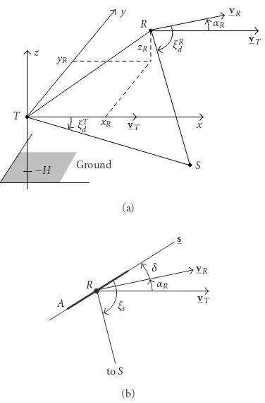
3. BISTATIC RADAR CONFIGURATION
The configuration geometry is shown inFigure 2. The trans-mitterTis at the center of an (x,y,z) coordinate system. The
x-axis points in the same direction as the velocity vectorvT of T. Thez-axis points vertically and up. The receiverRis located at (xR,yR,zR). Its velocity vectorvRis assumed to be horizontal and to make an angleαRw.r.t.vT. The linear an-tennaAis located atR. It is horizontal and makes an angle
δw.r.t.vR. The (bistatic) rangeRbto some scattererSis the distance fromT toStoR. The angular positions ofSw.r.t.
vT,vR, andsare denoted byξdT,ξdR, andξs, respectively. The ground is assumed to be a horizontal plane atz = −H. All scatterers corresponding to ground clutter are thus located in this plane. The magnitudes ofvT andvR are denoted by
vTandvR. Any bistatic configuration is fully characterized by the vector of (configuration) parameters
θ=H,xR,yR,zR,vT,vR,αR,δ
. (1)
4. DIRECTION-DOPPLER CURVES AND SURFACES
4.1. Important parameters
−H Ground S
Figure2: Bistatic radar configuration. (a) Transmitter (T)-receiver (R)-scatterer (S) geometry and related parameters. (b) Receiver an-tenna (A) and related angles.
delayτrt, the spatial frequencyfs, and the Doppler frequency
fd. For a stationary scatterer, we have τrt = Rb/c, fs = cosξs/λc, and fd =vr/λc, whereλcis the carrier wavelength andcis the speed of light.Rb,ξs, andvr are easily derived fromτrt,fs, andfd.
4.2. Isorange curves
All scatterersScharacterized by the same rangeRbare located on an isorange surface, which is an ellipsoid of revolution with foci atTandR. The intersection of this surface with the ground is an isorange curve, which is an ellipse (parameter-ized with polar angleψ).
4.3. 2D direction-Doppler curves
For any given configuration and range, all stationary scat-terersSat this range map onto a curve showing the relation between fsand fdfor any suchS. This curve is called a DD curve. DD curves are typically represented in terms of the normalized spatial frequency νs, equal to (λc/2)fs, and the normalized Doppler frequencyνd, equal to (λc/2(vR+vT))fd.
Figure 3shows that bistatic DD curves vary significantly with
configuration and range. The variation of these curves with range for any particular configuration is one of the most vis-ible manifestations of the RD problem.
To derive the equations of bistatic DD curves, we proceed as follows. First, we expressνdas a function ofνs. Since most DD curves have 2 distinct values ofνdfor mostνs’s, any DD
curve is best described by 2 functionsνd = f1(νs) andνd =
f2(νs), which describe the “bottom” and “top” parts of the curve, respectively.1Second, if we expressν
sandνdin terms of the angleψ, which also parameterizes the isorange ellipse, we find a parametric description of the DD curve, that is,
νs=g1(ψ) andνd =g2(ψ). The derivation of the fi(νs)’s and gi(ψ)’s is lengthy and thus omitted.
4.4. 3D direction-Doppler surfaces
We call the surface obtained by stacking DD curves for suc-cessive values ofRba DD surface.Figure 4shows the DD sur-face for the configuration ofFigure 3d.
4.5. Recovery of configuration parameters
Consider the DD surface S corresponding to an arbitrary bistatic configuration θ1 = (H,xR,yR,zR,vR,vT,αR,δ) and to all applicable values of Rb. One can show that the only other set of parameters that produces S is θ2 =
(H,xR,−yR,zR,vR,vT,−αR,−δ). Thus, the inverse problem of recoveringθfromShas2related solutions. We can then infer that the inverse problem of recoveringθfrom a single slice ofShasat least2 solutions and that at least 2 of them are related.
5. SNAPSHOTS
In each coherent processing interval, a coherent train ofM
pulses is transmitted fromT. The returns are sensed at each of theNelements of the linear antenna arrayAatR. Finally, the sensed returns are sampled at a number of discrete ranges (called range gates) covering the range interval of interest. Ranges are indexed withl∈L= {0, 1,. . .,L−1}. We regard the data as a sequence ofM×N2D data arrays (snapshots) at successive rangesl. TheM×Nsnapshot corresponding to a specificl(or even to some arbitrary value of the continu-ous range) and to a single scattererScharacterized by specific parameters (Rb,νs,νd) can be written as theMN×1 vector
MN×1 steering vector
vνs,νd vector. For uniform linear arrays, we have
aνs
1All curves have a bottom and a top, even when they appear flat, as in
−0.5 −0.4 −0.3 −0.2 −0.1 0 0.1 0.2 0.3 0.4 0.5
Figure3: Example of DD curves for four bistatic configurations and four rangesRb(170, 210, 250, and 400 km). Parameters specific to each configuration are (a) (xR,yR,zR)=(100, 0, 0) km,αR=0◦,δ=0◦, (b) (xR,yR,zR)=(0, 100, 0) km,αR =0◦,δ=0◦, (c) (xR,yR,zR)= (0, 100, 0) km,αR =90◦,δ =0◦, and (d) (xR,yR,zR)=(80, 50, 20) km,αR =35◦,δ =60◦. Common configuration parameters areH = −50 km andvR=vT=90 m/s.
The target snapshoty
tis directly given by (2), where we
c is a stochastic vector. We assume it is wide-sense stationary w.r.t. space and time. It is thus characterized by a constant CM Rc = E{y
cy
†
c}. Jammer snapshots are not considered here. The unavoid-able noise snapshot y
n is assumed to be uncorrelated with
y
c and to be spatially and temporally white and
indepen-dent of range. It is thus characterized by a constant CM
Rn=E{y
ny
†
n} =PnI, wherePnis the noise power. The im-portant quantity in STAP is the I + N snapshoty
q=yc+yn, characterized by the I + N CM
Rq=Ey
As alluded to earlier, the present paper differs from [7] primarily through the fact that, here, we use a set of sim-ulated, stochastic I + N snapshots y
−0.5
Figure 4: Example of DD surface for bistatic configuration of Figure 3d. RangeRb varies from 152 km to 350 km. Note that the minimum of 152 km is the smallest possible value forRb for this configuration.
6. OPTIMUM PROCESSOR
The structure of the optimum processor (OP) is shown in
Figure 5. The primary input is the snapshoty=y(l) at range
gatel(with rangeRb). Secondary inputs are specific values of
νsandνd and the theoreticalRq atl. The triplet (Rb,νs,νd) constitutes the “target hypothesis.” The weight vector that maximizes the output signal-to-interference-plus-noise ratio (SINR) is given by [11]
where α is an arbitrary complex constant. (Rb appears throughRq.) The detection statistic is the complex scalar
z=w†oνs,νd
y. (8) Its magnitude is compared to a threshold λ to determine whether the target hypothesis is true or false.
Rqin (7) is the theoretical I + N CM. In practice,Rqhas to be estimated from the data. This is discussed in the next section.
The performance of a processor using a weight w, whether optimal or not, is measured by the SINR loss defined as [2]
where SINR0is the SINR in the absence of clutter. Optimum performance is achieved for w = wo. Performance is de-graded by losses due to the estimation of the I + N CM (even in the absence of RD effects) and to inappropriate handling of the RD problem.
Target
Figure5: Structure of OP determining whether, for the giveny=
y(l), the target hypothesis (Rb,νs,νd) is true or false.
7. ESTIMATION OF I+N COVARIANCE MATRIXRq
At each rangel, one might be tempted to estimateRqvia [2]
whereNlis the number of snapshots used for estimation,Sl is the set of snapshot indiceskdefined byl−(Nl/2)< k <
l+ (Nl/2), andyq(k) is the snapshot at rangek. (Observe that rangelis omitted from the sum in (10).) However,Rq(l) is “maximum likelihood” only if they
q(k)’s are independent and identically distributed (i.i.d.) w.r.t. range and have com-plex Gaussian probability density functions (identical for all
k’s) [12]. Unfortunately, in virtually all configurations, the
y
q(k)’s arenoti.i.d. w.r.t. range. One of the clearest manifes-tations of this lack of stationarity w.r.t. range is the variation with range of the clutter PS and, in particular, of the clut-ter ridge. All these facts and issues are the essence of the RD problem in STAP.
If no RD compensation is performed, the estimateRq(l) in (10) provides reduced performance. The goal of any RD compensation method should be to produce the best possi-ble estimate forRq(l) based on the available data and in spite of the nonstationarity w.r.t. range. One such method is de-scribed below.
8. PRINCIPLE OF OUR REGISTRATION-BASED RANGE-DEPENDENCE COMPENSATION METHOD
We perform RD compensation by applying a properly de-signed transformation TklR[·] to each single-sample CM
At this point, TR
kl[·] should be regarded as a conceptual transformation. Its precise meaning will become clear later. Specifically, one should not assume it is a linear-transforma-tion matrix.
Since the nonstationarity is most visible in the spectral domain (via the deformation of the clutter ridge), we per-form the RD compensation in this domain, using the clut-ter ridges at the various ranges as guides. The transforma-tionTklR[·] is designed to deform the clutter PS at each range
k ∈ Sl to bring its clutter ridge into registration with that of the PS at reference rangel. Because of the direct relation between clutter ridges and DD curves, we can also think in terms of DD curves. The registration of DD curves is the key idea behind the method introduced in [7] and its general-ization presented here. Note that [5] also applies an elemen-tary form of registration, in that DD curves are brought into registration at their spectral centers, that is, at a single point only.
To implementTklR[·] in the spectral domain, we need an estimatePk(U,V) of the true PSPk(U,V). Here, we use the periodogram so that [13]
which we can write as follows:
Pk(U,V)=TklP Pk(U,V)
. (16)
From (12), (15), and (16), it is clear that it would be ex-tremely difficult to expressTP
kl[·] in terms ofTklR[·]. There-fore,TklP[·] should only be interpreted as a conceptual trans-formation, just asTklR[·] should be.
Pk(U,V) in (12) is also the 2D DTFT of the estimate
Γq,k[lm,ln] of the 2D statistical autocorrelation sequence of the snapshot y
q(k). Denoting by yq,k(m,n) the 2DM×N array representing the realization at hand ofyq(k), we have
θ compensation (RBC)Registration-based
Γq(k)
(a)
Γq(k) θ compensation (RBC)Registration-based
Figure6: The subsystem for properly transforming the reduced-size CMΓq(k) intoΓq(k) can operate in (a) TP mode (for knownθ)
or (b) EP mode (for estimatedθ). In both cases, the transformation is performed by the common RBC module. In the second case, the unknown configuration parameters are provided by the CPE mod-ule. Note that the current CPE module usesallinputsΓq(l), that is, ally advantageous to perform the compensation usingΓq(k)
rather thanRq(k).
The transformationTklΓ[·] is not given in analytical form, but as an algorithm operating on the inputΓq(k) and
pro-ducing the outputΓq(k).Figure 6shows two possible imple-mentations ofTklΓ[·], depending upon whether we know the configuration-parameter vectorθor we have to estimate it. These modes of operation are respectively called TP and EP.
Figure 6 highlights the presence of two key processing
modules: RBC and CPE. The RBC module is used in both modes of operation and transformsΓq(k) using either the
Angle-Doppler domain
Peak extraction (1)
at rangek
Mapping from rangek
to rangel
Interpolation
P(k) Configuration parametersθorθ P(k)
2D FFT 2D IFFT
Γp(k) Γp(k)
Space-time domain
Expansion and zero-padding
(Only fork < l) Windowing
Γq(k) Γq(k)
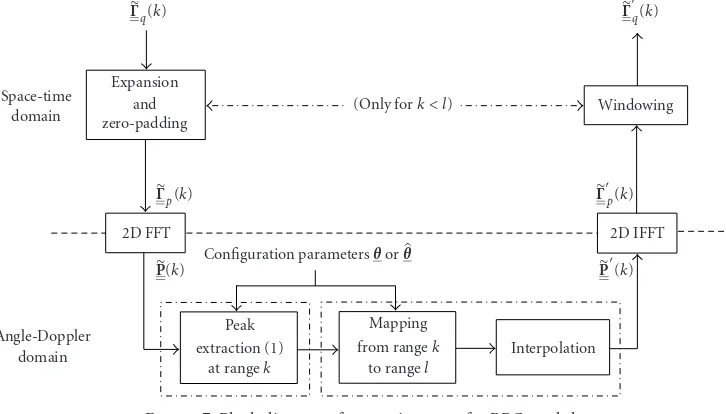
Figure7: Block diagram of processing steps for RBC module.
DD surface fitting θ · · · ·
Angle-Doppler domain
Peak extraction
(2) · · ·
Peak extraction
(2) · · ·
Peak extraction (2)
P(0) P(l) P(L−1)
2D FFT 2D FFT 2D FFT
Γp(0) Γp(l) Γp(L−1)
Space-time domain
Expansion and zero-padding
· · ·
Expansion and zero-padding
· · ·
Expansion and zero-padding
Γq(0) Γq(l) Γq(L−1)
Figure8: Block diagram of processing steps for CPE module.
In spite of the added degree of difficulty in the problem considered here (as compared to that considered in [7]), the RBC module described in [7] is directly applicable here. Its block diagram is shown inFigure 7, but the reader is referred to [7] for additional details.
In contrast, the CPE module of [7] needs a major over-haul to deal with the increased degree of uncertainty consid-ered here and illustrated inFigure 1.
9. CONFIGURATION-PARAMETERS
ESTIMATION MODULE
Figure 8shows the block diagram of the CPE module. This
diagram is a generalization of the corresponding diagram in [7]. One main difference is that the PS for all rangesl∈L
are used. The Γq(l)’s are processed individually up to and including peak extraction (described in Section 10). The peaks corresponding to all l’s are then used jointly to find the DD surface that best matches them. This surface yields the estimateθofθ.
The significant contributions of this paper are the de-sign and evaluation of the peak extraction (2) and of the DD-surface-fitting processing steps (i.e., algorithms) shown inFigure 8.
Figure 1ashows the PS obtained for a givenθand a given
−0.5 −0.3 −0.1 0.1 0.3 0.5
νs
−0.5
−0.4
−0.3
−0.2
−0.1
0 0.1 0.2 0.3 0.4 0.5
νd
(a)
−0.5 −0.3 −0.1 0.1 0.3 0.5
νs
−0.5
−0.4
−0.3
−0.2
−0.1
0 0.1 0.2 0.3 0.4 0.5
νd
(b)
Figure9: Each subfigure shows the peaks extracted at a given range by the peak extraction (2) algorithm. The underlying, theoretical DD curve is also shown. Whereas, in (a), the extracted peaks are very close to the underlying DD curve, in (b), they tend to fall fur-ther away, which leads to inaccuracies in the DD-surface-fitting al-gorithm.
stochastic snapshotyq. From one realization to the next, the PS estimate and, thus, the related clutter ridge will most likely change. However, this clutter ridge will always be located in the vicinity of the underlying DD curve, which is the same as in the 1st case. Comparing both cases, it is clear that the 2nd is more challenging since we may experience difficulties in extracting the peaks and in fitting a DD surface to them.
The reader is referred to [7] for a description of the first two processing steps, that is, expansion and zero-padding and 2D FFT. In fact, these steps are identical to the first two steps of the RBC module (Figure 7). In both cases, the pur-pose of these steps is to bring us into the spectral domain. (The expansion sizes associated with the 2D FFT may differ in both modules.)
−0.5
0 0.5
νs
−0.5
0
0.5
νd 0
50 100 150
Rb
Figure10: 3D scatter plot of extracted peak locations in (νs,νd,Rb )-axes. The peak locations shown are located in theLhorizontal slices corresponding to theLvalues ofl∈L. The locations in each slice are the output of the peak extraction (2) algorithm. The complete collection of peak locations is the input to the DD-surface-fitting algorithm. Ideally, these points should fall on the underlying DD surface. In practice, they should most likely fall in its vicinity.
The other two processing steps, that is, peak extraction (2) and DD surface fitting, are described in the next two sec-tions. Their design, implementation, and evaluation are the major contributions of this paper.
10. PEAK EXTRACTION (2) ALGORITHM
The corresponding algorithm of [7] was significantly modi-fied to deal with the sparsity and stochastic behavior of the peaks in any given realization of a PS. The new algorithm for extracting the desired peaks from the PS at any given rangel
works as follows: (1) the largest value PSmax in the PS array is found; (2) allpixelsin the PS array with values less than a given percentage (set here to 30%) of PSmax are set to zero; (3) the remaining nonzero values are grouped into regions by the “connected components” labelling technique of im-age processing [14] or equivalent; (4) the largest value within each region is found and the location of the corresponding pixel defines the location of the peak for that region.
This peak-extraction algorithm is based on the hope that the largest value in each region will fall on or close to the underlying DD curve. Simulations show that this is generally the case. This is illustrated inFigure 9.
The above algorithm is then applied to eachl∈L. This leads to a constellation of peak locations, as illustrated in Fig-ures10and11. This constellation of points is the input to the DD-surface-fitting algorithm.
11. DD-SURFACE-FITTING ALGORITHM
−0.5 0 0.5
νs
−0.5
0 0.5
νd
(a)
−0.5 0 0.5
νs
−0.5
0 0.5
νd
(b)
−0.5 0 0.5
νs
−0.5
0 0.5
νd
(c)
−0.5 0 0.5
νs
−0.5
0 0.5
νd
(d)
Figure11: Each subfigure is the top view of a 3D scatter plot of peak locations similar to that ofFigure 10. The four subfigures labelled (a) through (d) correspond to the configurations of Figures3a–3d, respectively.
For purpose of conciseness, we limit ourselves here to de-scribing its general principle.
We start from the 3D constellation of points (extracted peak locations) that can be thought of as lying on an experi-mentalDD surface that, we hope, approximates well the un-derlying theoretical DD surface. Our goal is to recover the set of configuration parameters that characterizes this theo-retical DD surface (Figure 2). (We know that there may be 2 such sets and that they are related.) Since it is quite logical to assume that we knowHandvR, we only need to estimatexR,
yR,zR,vT,αR, andδ. First, we derive the tightest possible con-straints on the possible values ofxR,yR, andzRto reduce the search space. Then, we explore each allowed position (xR,yR) and estimate the other parameters.
11.1. Determination of constraints onxR,yR, andzR We apply the same method as in [7]. However, the sparsity of the estimated peak locations prevents us from directly ob-taining the estimatesνmin
s,l andνmaxs,l of the extremities, along theνs-axis, of the DD curve at eachl. We have thus devel-oped a new method to derive reliable estimatesνmins,l andνmaxs,l
at eachlby taking into account the set of peaks for alll’s in L. Results have proven to be more accurate at shorter ranges
Rb. Therefore, we focus on a single short range (typically for
l =4 rather than forl=0 to improve accuracy) and deter-mine the constraints onxR,yR, andzRexactly as in [7].
11.2. Determination ofzR,vT,αR, andδfor each(xR,yR) As in [7], we apply the following procedure to each allowed pair (xR,yR). First, we computezR using a formula we have derived, which relateszRtoxR,yR,νsmin,l , andνmaxs,l . This for-mula is quite lengthy and is thus omitted. IfzR satisfies the constraints specified in [7], we proceed. Otherwise, we dis-card the candidate pair. To proceed, we rely on exact analyti-cal expressions for DD surfaces in terms ofθ.2For each can-didate position (xR,yR,zR) ofR, we first insert the values of (xR,yR,zR) in the analytical expressions for the DD surface.
2Deriving these equations is quite complicated. Furthermore, the
OP TP SAP
−0.5 −0.4 −0.3 −0.2 −0.1 0 0.1 0.2 0.3 0.4 0.5
νd
−60
−50
−40
−30
−20
−10
0
SINR
L
(dB)
Figure12: The end-to-end performance of a STAP processor using RBC and working in TP mode (knownθ) is a direct reflection of the performance of the RBC module (seeFigure 6). Performance is shown in terms ofcutsof SINR loss atνs=0. The performances of the OP (the best achievable) and of the straight-averaging processor (no RD compensation) are also shown as references.
Then, we estimate the remaining unknown parametersvT,
αR, andδby least-square fit of the resulting parametric sur-face to the extracted peak locations. We have found that the upper part of the DD surface is better suited for estimating
vT,αR, andδ. As a result, we perform the fitting using only theNlr longest ranges. The resulting least-square fit error is also computed. The influence of the choice of value forNlris discussed inSection 12.2.
11.3. Final parameter selection
The procedure just described (inSection 11.2) is repeated for all allowed pairs (xR,yR). The set of parameters resulting in the smallest least-square fit error is ultimately chosen. These parameters, as well as the knownHandvR, make up the final θ.
12. PERFORMANCE EVALUATION
We first discuss the individual performances of the RBC and CPE modules. Then, we compare the end-to-end perfor-mance of STAP processors working in TP mode and in EP mode to those of the OP and of the straight-averaging pro-cessor (no compensation).
12.1. Performance of RBC module
To evaluate the individual performance of the RBC module, we consider an end-to-end STAP processor using RBC and working in TP mode. Indeed, this mode of operation only involves the RBC module (seeFigure 6). The performance of this processor is shown in Figure 12in terms of SINR loss plots.
−0.5 −0.4 −0.3 −0.2 −0.1 0 0.1 0.2 0.3 0.4 0.5
νd
−50
−45
−40
−35
−30
−25
−20
−15
−10
−5
0
SINR
L
(dB)
pincreases
N=M=12
(a)
−0.5 −0.4 −0.3 −0.2 −0.1 0 0.1 0.2 0.3 0.4 0.5
νd 1
20 OP
Expansion
coe
ffi
cient
p
(b)
Figure13: Cuts of SINR loss atνs=0 for various values of expan-sion coefficient p. OP is shown for reference. (a) Topmost curve corresponds to OP. Other curves, from bottommost to topmost, correspond to pincreasing from 1 to 20. (b) Alternate visualiza-tion, where grayscale corresponds to SINR loss. Curves are shown in the same order as in (a), with topmost row corresponding to OP. Performance increases with increasingpand gets very close to that of OP for largep.
With reference to Figures 7 and8, recall that we must typically expand the size of Γq(k) when the source range
k is smaller than the destination range l. This is done by zero-padding. The relative size of this padding plays a crit-ical role in the performance of the RBC module. To char-acterize this expansion, we define the expansion coefficients
p=P/(2M−1) andq=Q/(2N−1), whereP,Q,N, andM
are related to the sizesP×Qand (2M−1)×(2N−1) ofΓp
andΓq, respectively. In our experiments, all arrays are square and, thus,p=q.
Figure 13 illustrates the influence of p on the SINR
−0.6
Figure14: Four different views of the true DD surface color coded with the absolute value of the fit error for the configuration ofFigure 3c.
for νs = 0. The topmost curve corresponds to the OP, while the other curves, from bottommost to topmost, cor-respond to processors using values of p increasing from 1 to 20. Figure 13bprovides an alternate visualization of the same information as in Figure 13a: the vertical axis now corresponds to p and the grayscale to SINRL. Both plots clearly show that performance increases with p. Further-more, performance for large p’s gets very close to that of the OP.
Getting close to OP performance with stochastic snap-shots implies using a large p, which leads to significant computational requirements. However, this is counterbal-anced by a reduction of the sample-support size, Nl. In-deed, the results shown in Figure 13 were obtained with only Nl = 32 snapshots, whereas the rule of Reed, Mal-lett, and Brennan (RMB) [15] requires at least 288 snap-shots for M = N = 12. Figure 13a shows the im-provement over the 3 dB loss associated with the RMB rule.
12.2. Performance of CPE module
To evaluate the individual performance of the CPE module, we pick some parameterθ, generate corresponding stochas-tic snapshotsy
q(l),l∈ L, run the CPE algorithm, and ex-amine the outputθ. We then compute the (absolute value of the) “horizontal” (i.e., in the (νs,νd)-plane) fit error between the estimated DD surface corresponding to θ and the true DD surface corresponding toθ.Figure 14shows the errors as colors on the true DD surface. Observe that the largest er-rors occur at short ranges, this is because DD curves change more rapidly with range at short ranges than at long ranges.
Figure 15shows the RMS horizontal error between estimated
OP TP
EP SAP
−0.5 −0.4 −0.3 −0.2 −0.1 0 0.1 0.2 0.3 0.4 0.5
νd
−45
−40
−35
−30
−25
−20
−15
−10
−5
0
SINR
L
(dB)
(a)
OP TP
EP SAP
−0.5 −0.4 −0.3 −0.2 −0.1 0 0.1 0.2 0.3 0.4 0.5
νd
−50
−45
−40
−35
−30
−25
−20
−15
−10
−5
0
SINR
L
(dB)
(b)
OP TP
EP SAP
−0.5 −0.4 −0.3 −0.2 −0.1 0 0.1 0.2 0.3 0.4 0.5
νd
−45
−40
−35
−30
−25
−20
−15
−10
−5
SINR
L
(dB)
(c)
OP TP
EP SAP
−0.5 −0.4 −0.3 −0.2 −0.1 0 0.1 0.2 0.3 0.4 0.5
νd
−60
−50
−40
−30
−20
−10
0
SINR
L
(dB)
(d)
Figure15: Each subfigure quantifies the end-to-end performance of TP, EP, OP, and SAP processors for a given configuration. The four subfigures correspond to the four configurations ofFigure 3. Each subfigure shows cuts of SINR loss atνs=0 for the OP (topmost curve), SAP (bottommost curve), and TP and EP (middle curves, with TP above EP). Conclusions drawn from the graphs are given in the text.
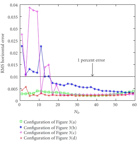
Figure 16shows the RMS horizontal error between the
estimated and true DD surfaces as a function of the number of “long ranges,”Nlr. We see that an acceptable fit is obtained for relatively small values ofNlr. This is significant since a reduction inNlrresults in a reduction of the computational load.
12.3. End-to-end performance
1 percent error
Configuration of Figure 3(a) Configuration of Figure 3(b) Configuration of Figure 3(c) Configuration of Figure 3(d)
0 10 20 30 40 50 60
Nlr 0
0.005 0.01 0.015 0.02 0.025 0.03 0.035 0.04
RMS
hor
iz
o
ntal
er
ro
r
Figure16: RMS horizontal error (between estimated and true DD surfaces) as a function of the number oflong ranges,Nlr, used by the DD-surface-fitting algorithm for the four configurations ofFigure 3. In all cases, the errortendsto decrease with increasingNlr. However, past aboutNlr=15, there is little improvement.
Table1: RMS horizontal error between estimated and true DD sur-faces.
Configuration RMS horizontal error (unitless)
Figure 3a 0.0024
Figure 3b 0.0062
Figure 3c 0.0026
Figure 3d 0.0019
processor (SAP; no RD compensation) are also shown for reference.Figure 15shows the SINR loss curves correspond-ing to the TP, EP, OP, and SAP processors for the four config-urations ofFigure 3. The plots show that the performance of TP is close to that of OP and much better than that of SAP, thereby demonstrating the soundness of our registration-based approach to RD compensation. The plots also show that EP performance is close to that of TP, thereby demon-strating the soundness of our combined peak extraction and DD-surface-fitting approaches for estimating the configura-tions parameters.
13. CONCLUSION
The range-dependence (RD) problem in STAP originates from the lack of stationarity of the snapshot statistics w.r.t. range. Its clearest manifestation is the deformation with range of the power spectrum. The usual maximum
likeli-hood estimate of the interference-plus-noise covariance ma-trix (CM)Rqis no longer optimal and leads to poor target-detection performance. Therefore, it becomes imperative to develop RD compensation methods.
In [7], we introduced registration-based methods for knownRq and developed a general strategy for estimating the CM at each range. This strategy is based on the registra-tion of clutter ridges and direcregistra-tion-Doppler (DD) curves at each range, using known (theoretical) CMsRqat neighbor-ing ranges.
In this paper, we adapted the strategy of [7] to handle single realizations of stochastic snapshots. The main diffi-culty lies in the estimation of the configuration parameters. The main contributions of this paper are the modification of the peak-extraction algorithm of [7] and the development of a new 3D DD-surface-fitting algorithm generalizing the 2D DD-curve-fitting algorithm of [7]. The performance of the new algorithms was evaluated in detail.
ACKNOWLEDGMENTS
REFERENCES
[1] R. Klemm,Principles of Space-Time Adaptive Processing, vol. 9 ofRadar, Sonar, Navigation & Avionics, IEE, London, UK, 2002.
[2] J. Ward, “Space-time adaptive processing for airborne radar,” Tech. Rep. 1015, MIT Lincoln Laboratory, Lexington, Mass, USA, 1994.
[3] G. K. Borsari, “Mitigating effects on STAP processing caused by an inclined array,” inProc. IEEE National Radar Conference (RADARCON ’98), pp. 135–140, Dallas, Tex, USA, May 1998. [4] S. M. Kogon and M. A. Zatman, “Bistatic STAP for airborne radar systems,” inAdaptive Sensor Array Processing Workshop, MIT Lincoln Laboratory, Lexington, Mass, USA, March 2000. [5] B. Himed, Y. Zhang, and A. Hajjari, “STAP with angle-Doppler compensation for bistatic airborne radars,” inProc. IEEE National Radar Conference (RADARCON ’02), pp. 311– 317, Long Beach, Calif, USA, April 2002.
[6] W. L. Melvin, B. Himed, and M. E. Davis, “Doubly adaptive bistatic clutter filtering,” inProc. IEEE National Radar Con-ference (RADARCON ’03), pp. 171–178, Huntsville, Ala, USA, May 2003.
[7] F. D. Lapierre, J. G. Verly, and M. Van Droogenbroeck, “New solutions to the problem of range dependence in bistatic STAP radars,” inProc. IEEE National Radar Conference (RADAR-CON ’03), pp. 452–459, Huntsville, Ala, USA, May 2003. [8] F. D. Lapierre and J. G. Verly, “Registration-based solutions to
the range-dependence problem in STAP radars,” inAdaptive Sensor Array Processing Workshop, MIT Lincoln Laboratory, Lexington, Mass, USA, March 2003.
[9] F. D. Lapierre, M. Van Droogenbroeck, and J. G. Verly, “New methods for handling the range dependence of the clut-ter spectrum in non-sidelooking monostatic STAP radars,” inProc. IEEE Int. Conf. Acoustics, Speech, Signal Processing (ICASSP ’03), vol. 5, pp. 73–76, Hong Kong, April 2003. [10] S. D. Hayward, “Adaptive beamforming for rapidly moving
arrays,” inProc. IEEE International Radar Conference, pp. 480– 483, Beijing, China, October 1996.
[11] L. E. Brennan and I. S. Reed, “Theory of adaptive radar,”IEEE Trans. on Aerospace and Electronic Systems, vol. 9, no. 2, pp. 237–252, 1973.
[12] N. R. Goodman, “Statistical analysis based on a certain mul-tivariate complex Gaussian distribution (an introduction),” Annals of Mathematical Statistics, vol. 34, no. 1, pp. 152–177, 1963.
[13] D. G. Manolakis, V. K. Ingle, and S. M. Kogon,Statistical and Adaptive Signal Processing, McGraw-Hill, New York, NY, USA, 2000.
[14] D. Ballard and C. Brown, Computer Vision, Prentice-Hall, Englewood Cliffs, NJ, USA, 1982.
[15] I. S. Reed, J. D. Mallett, and L. E. Brennan, “Rapid conver-gence rate in adaptive arrays,” IEEE Trans. on Aerospace and Electronic Systems, vol. 10, no. 6, pp. 853–863, 1974.
Fabian D. Lapierrewas born in Huy, Bel-gium. He received the Ingenieur Electroni-cien (Electronics Engineer) degree from the University of Li`ege, Belgium, in 2000. In the same year, he received a fellowship of the Fonds National de la Recherche Scientifique (FNRS), Brussels, Belgium, to work on a Ph.D. thesis. He is in his final year as a Ph.D. student. His research interest is mainly fo-cussed on space-time adaptive processing (STAP) for bistatic radars.
Jacques G. Verly was born in Li`ege, Bel-gium. He received the Ingenieur Electron-icien (Electronics Engineer) degree from the University of Li`ege, Belgium, in 1975. Through a sponsorship of the Belgian American Educational Foundation (BAEF), he joined Stanford University, Stanford, Calif, where he received the M.S. and Ph.D. degrees in electrical engineering in 1976 and