R E S E A R C H
Open Access
A novel modified Omega-K algorithm for circular
trajectory scanning SAR imaging using series
reversion
Yi Liao
*, Meng-dao Xing, Lei Zhang and Zheng Bao
Abstract
This article presents a modified Omega-K algorithm for circular trajectory scanning synthetic aperture radar (CTSSAR) imaging. Due to the curvature of circular trajectory, it is difficult to have access to the two-dimensional frequency spectrum for CTSSAR via the principle of stationary phase (POSP), as conventional SAR imaging methods RD and CS. Herein, the analytic point target spectrum is first derived by series reversion and the POSP, based on which a modified Omega-K algorithm is developed to focus data accurately. The accuracy can be controlled by keeping enough terms in the two series expansions so that a well-focused image can be achieved with a proper range approximation. After detailed analyses and experiments, the fourth-order approximation is proved to be the best choice. Furthermore, the computational efficiency is evaluated by comparing the given method with the back projection algorithm and other methods with different approximated orders. The proposed algorithm is verified to be the best one in terms of computational burden. A well-focused image is obtained by simulations, validating the feasibility of the proposed algorithm.
Keywords:Circular trajectory scanning (CTS) synthetic aperture radar (SAR) (CTSSAR), Series reversion, Omega-K algorithm
1. Introduction
Due to its capability of working day/night and all weather conditions, synthetic aperture radar (SAR) has widely been applied to the military and civilian practical uses. The traditional SAR system often operates along a straight path at a certain altitude with respect to the ground plane [1-4]. In recent years, the curved path SAR has attracted more and more attention of many re-searchers. An imaging mode called circular SAR (CSAR), whose radar system moves along a circular trajectory, gradually became one of the hotspots in the field of radar signal processing [5]. In CSAR imaging mode, the sensor steers its antenna beam to illuminate a certain terrain patch, like “circular spotlight” mode to some ex-tent. CSAR owns many advantages over the conven-tional one that it has the capability to achieve sub-wavelength resolution in the ground plane due to its aperture of 360°. What is more, the multi-aspect
observation of CSAR provides the information of the in-terested target from different azimuth directions, making it possible to realize a 3D reconstruction [6-14]. Al-though CSAR owns so many advantages, the imaging area is relatively small. Usually, both the height and the diameter of the imaging area in the ground plane are several hundred meters [15]. Therefore, it is suitable for the high-resolution imaging of an interested area.
A new wide area circular trajectory scanning SAR (CTSSAR) imaging mode has raised the interests of a growing numbers of researchers [16]. In this mode, the platform moves along a circular path at a certain altitude with its antenna beam pointing fixed perpendicular to the flight velocity away from the center of the circular trajectory, the result is a moving antenna footprint that sweeps along an annular terrain. Just like the spotlight SAR and CSAR, the only thing differs CTSSAR from the conventional stripmap is the shape of the track. Hence, we prefer to call CTSSAR as‘circular stripmap’similarly. Although certain sacrifices in azimuth resolution may occur, CTSSAR can possess a larger imaging area than * Correspondence:[email protected]
National Key lab of Radar Signal Processing, Xidian University, Xi’an 710071, P.R. China
that of the traditional stripmap mode for its higher scanning speed in azimuth, so it is more suitable for fast wide area imaging.
Due to the trajectory curvature of CTSSAR, there are trigonometric functions under the radical sign in the target’s range function. The accurate analytical expres-sion of the 2D spectrum is not achievable by adopting conventional principle of stationary phase, which becomes an obstacle in the way of designing a fast
frequency-domain-based algorithms for CTSSAR imaging. Thus, Sun et al. [16] employ a quadratic approximation to the range function in its deduction of the spectrum to design an imaging method. In the case that the synthetic aperture is relatively short and the azimuth resolution is low, the impact of the curved trajectory can be neglected, and sat-isfactory results can be reached using this method. Never-theless, the quadratic approximation method ignores the high-order range terms. Under the condition that the
p
r
a
r
ω
( ) Rη c
H
r
θ
O′
p
θ
θ
(
rpcosθp,rpsinθp, 0)
(racos ,θrasin ,θHc) p
θ θ= +ωη
a
r p
θ
Y
X
integration time is long and the azimuth resolution is high, the range errors introduced by this approximation will be large enough to defocus the image. The back projection (BP) algorithm shown in [10] is a classical time-domain algorithm, which can get rid of the problem of spectrum derivation in the frequency-domain-based algorithms and be implemented easily with arbitrary geometries. But the disadvantage is that each pixel must be compensated individually, leading to a heavy computational burden.
In order to obtain a more applicable approach to focus CTSSAR data, a novel imaging algorithm for CTSSAR is proposed based on the method of series reversion (MSR). The MSR is a method using the Doppler series expansion coefficients to obtain the coefficients of the stationary phase by reversion [17,18]. The accuracy of the spectrum is controlled by keeping enough terms in the two series expansions. Moreover, the corresponding modified Omega-K algorithm is established based on the derived 2D spectrum.
In this article, the imaging geometry model is analyzed first and the involved problem is discussed as well. To obtain the 2D spectrum based on MSR, the range function is kept up to the fourth-order. Thus, a new modified Omega-K algorithm tailored for CTSSAR over a circular path is developed and the detailed flowchart is given. Finally, the algorithm is tested with satisfying results by simulations for point targets in different range. Imple-mentation aspects, including resolutions, computational complexity, and the sensitivity to motion errors, are also assessed in this article.
2. Signal model for CTSSAR
The imaging geometry for CTSSAR is shown in Figure 1. The radar platform moves along a circular path of radius
rawith heightHcon a plane parallel to the ground plane. As the radar moves, its beam is in the plane perpendicular to the flight velocity all the time. When the radar platform moves around a whole circle centered at the origin point O of the spatial coordinate, the beam-illuminating scene will be an annular area with inner radius OB and outer radius OC. The coordinate of radar platform A is denoted by (ra cos θ, ra sin θ, Hc), where the aspect angle is θ. Assume that there is an arbitrary point targetPlocated at (rp cos θp, rp sin θp, 0). For simplicity of the following derivation, let us define that the slow time is zero when
θ=θp, namely, the beam center crossing time. The angle velocity is denoted byω, and the slow time is represented by η. So, we haveθ = θp +ωη. Thus, the instantaneous range R(η) between the radar and the target P can be obtained based on the law of cosines as shown in the following expressions.
Defining Rcen¼
ffiffiffiffiffiffiffiffiffiffiffiffiffiffiffiffiffiffiffiffiffiffiffiffiffiffiffiffiffiffiffiffi
H2
c þ rpra
2
q
, we perform Taylor expansion to the instantaneous range neglecting the terms whose order are higher than the fourth order. The expression can be written as
Rð Þ ¼η Rcenþk1ηþk2η2þk3η3þk4η4þK ð3Þ
Assume that the transmitting radar signal is linear frequency modulation signal, the pulse width isTp, and the rate of frequency modulation is γ. The echo from P
can be presented by
srðt;ηÞ ¼σpar t are the range envelope and azimuth envelope, respectively,
cis the speed of light, and λis the wavelength according to the center frequency.
Now, convert the echo signal shown in (5) to the range frequency azimuth time domain,
S0ðfτ;ηÞ ¼σpArð Þfτ aað Þη :exp j
wherefcis the carrier frequency,fτis the range frequency,
andAr(fτ) represents the envelope of the range frequency.
Now let us try to figure out the 2D spectrum using the stationary phase method as follow, first azimuth FFT is performed to (6), yielding
The phase in the Fourier integral is
θ ηð Þ ¼ 4πðfcþfτÞRð Þη
c
πfτ2
γ 2πfηη ð8Þ
Then operate on the derivatives ofθ(η) with respect to the components ofη,
dθ ηð Þ
Let it be zero, yielding
fη ¼ 2ðfcþfτÞωrarpsinωη
c ffiffiffiffiffiffiffiffiffiffiffiffiffiffiffiffiffiffiffiffiffiffiffiffiffiffiffiffiffiffiffiffiffiffiffiffiffiffiffiffiffiffiffiffiffiffiffiffiffiffiffiffiffiffir2 aþHc2þrp22rarpcosωη
q ð10Þ
From (9), it can be noticed that there are trigonometric functions in both numerator and denominator of the azi-muth Doppler frequency, which will make the deduction ofηby (9) very hard to carry out and further put a huge obstacle in the way of deriving the accurate 2D spectrum. This problem is caused by the curvature of the circular trajectory in CTSSAR. Thus, enough approximation is required to derive the 2D frequency spectrum and ensure a satisfied focusing result. Sun et al. [16] proposed a quad-ratic approximation method to make the spectrum expres-sion similar to that of the traditional straight line stripmap mode. This approach ignores the curvature of the circular trajectory and the parabolic approximation is introduced, making the spectrum derivation relatively easy to imple-ment. However, the precision of the obtained spectrum is relatively lower. In case of low-resolution and short inte-gration time, i.e., when the impact of the curvature of the motion trajectory to the range variation can be neglected, the flight path for the target point can be regarded as straight line approximately. Thus, the method in [16] is suitable under this situation. Nevertheless, if the integra-tion time is relatively long and the required azimuth resolution is high, the image might show significant deg-radation by adopting the original quadratic approximation method for its neglecting of the high-order terms. So, it is necessary to find a new spectrum deducing method for CTSSAR.
3. 2D spectrum and imaging algorithm
3.1. The deduction of the 2D spectrum based on MSR From the above analysis, it is obvious that due to the complicated range expression in the CTSSAR where the simple quadratic range equation does not hold, the sta-tionary phase point is difficult to approach and the 2D spectrum is hard to obtain. Thus, MSR is adopted to deduce the 2D spectrum, and the stationary phase
point’s series expansion coefficients with respect to azimuth time will be estimated by reversing the coeffi-cients in the Doppler spectrum, and the high accuracy 2D spectrum will be obtained. In the procedure of deduction, the accuracy of the deduced spectrum can be controlled by choosing an approximating order in the expansion, which will be discussed in detail in Section 4. In addition, the effective algorithm for CTSSAR will be designed based on the spectrum.
As for (9), let the derivative be zero [16], and the Doppler frequency can be written as follows:
c
fcþfτ
fη¼2k2ηþ3k3η2þ4k4η3þL ð11Þ
Using MSR, we can get the azimuth time in the form of Doppler frequency expansion, i.e., the expression of the stationary phase point which is presented as follows:
η fη ¼A1 c
According to (6) and (12), it is easy to get the following equation
where Aa(fη) is the envelope of the Doppler frequency. What should be pointed out here is that the odd terms are zero due to the trigonometric functions in the range equa-tion. It is necessary to keep (14) to a certain order when the image is well focused. The analysis of it will be mentioned in detail in Section 4. Moreover, according to (12), (13) and (14), the phase in the 2D spectrum of the target point signal can be rewritten as follows:
S2df fτ;fη
and the phase term in (15) can be shown as follows:
In (16), the phase in the 2D spectrum is kept up to the fourth-order with respect to fη, and a more precise
spectrum is obtained. Herein, the third term on the right-hand side of the equal sign indicates the curvature of the circular trajectory. In the following section, the imaging algorithm for CTSSAR will be given based on the 2D spectrum derived by the above analysis.
3.2. Imaging algorithm
Our objective is to obtain the frequency-domain signal containing the linear terms of the target only. It can be seen from the above deduction that there are variables such as fτ, fη, and R(η) in the spectrum. Due to the
existence of the coupling between the range frequency
fτand the Doppler frequencyfηin the 2D spectrum, it
is not easy to get the separated linear frequency term. Herein, the Taylor series expansion of (16) is operated infτ= 0, i.e.,
θc¼
4πðfcþfτÞRcen
c þφaz fη þφrcm fη fτ
þφsrc fη fτ2þφrgð Þ þfτ φres fη;fτ
ð17Þ
where4πfτRcen
c is the linear phase representing the loca-tion of target point, where the energy of the target can be focused within the corresponding range cell. 4πfcRcen
c is the constant term, which is independent from fτand fη, so its influence to the focusing can be omitted. In
addition, the other five terms can be shown as follows: a.Azimuth modulation term: The second phase term on the right-hand side of the equal sign of (17) is the azimuth modulation term, i.e.,
φaz fη ¼
π:c:f2 η 4k2fc
πk4c
3f4 η 64k4
2fc3
ð18Þ
This term indicates the azimuth modulation. The azi-muth modulation rate is range-variant for the fact that thek-coefficients are varied with range cells. The coup-ling between range and azimuth cannot be removed in the 2D frequency domain, so the term must be compen-sated in the range/Doppler domain. Herein, the azimuth compression is completed by multiplying the signal with the azimuth match filtering function after range cell migration (RCM) and range compression.
Azimuth partition Raw data
Two dimensional FFT
Two dimensional FFT
Two dimensional FFT
1( , , 0)
H f f R H1(f,f R, 0) H1(f,f R, 0)
Range IFFT
Range IFFT
Range IFFT
2 , , cen
H f f R H2 f,f R, cen H2 f,f R, cen
Azimuth IFFT
Azimuth IFFT
Azimuth IFFT
Geometric correction
Geometric correction
Geometric correction
Image mergence
SAR image
b. RCM term:
The third phase term on the right-hand side of the equal sign of (17) is the RCM term, i.e.,
φrcm fη ¼
π:c
4k2
fη fc
2
þ3πk4c3
64k4 2
fη fc
4
ð19Þ
This term varies withfη, representing the coupling between the range and the azimuth which needs to be compensated. For the common case of CTSSAR imaging, the range swath is not so wide that the RCM term’s range variation can be neglected. In the following process, the scene center is chosen as the reference and the corresponding RCM correction function is established in the 2D frequency domain to realize the range migration correction.
c. Secondary range compression term (SRC):
The fourth phase term on the right-hand side of the equal sign of (17) is the SRC term, i.e.,
φsrc fη ¼
π:C:f2 η
4k2fc3
3πk4c
3f4 η
32k4 2fc5
ð20Þ
This term indicates the variation of the range modulation rate resulted from the coupling between fτandfη. So, this term will impact the range focusing if not considered properly, while the variation of the SRC with range can be neglected usually. Thus, the compensated term in the 2D frequency domain is built with the scene center the reference to remove the influence of the SRC term to imaging.
d. Range modulation term:
The fifth phase term on the right-hand side of the equal sign of (17) is the range modulation term, i.e.,
φrgð Þ ¼ fτ
πf2 τ
γ ð21Þ
This term presents the range modulation of the transmitted signal, which is independent fromfη. It can be compensated in the 2D frequency domain as well.
e. Residue phase term:
The sixth phase term on the right-hand side of the equal sign of (17) is the residue phase term, i.e.,
φres fη;fτ
¼ π:c:f
2 η
4k2
f3 τ f3
cðfcþfτÞ
πk4c
3f4 η
64k4 2
1=ðfcþfτÞ 1=fc3þ3fτ=fc46fτ2=fc5
ð22Þ
This term indicates the high-order residue phase which will be compensated in the 2D frequency domain.
Therefore, according to the above analysis, it is pos-sible to acquire the thinking of the modified Omega-K method. Based on the 2D spectrum expression of the SAR echo signal shown in (15) and (16), first the phase
of the echo signal is coarsely compensated by
performing match filtering for the center point and then the residual range-variant phase is compensated in range Doppler domain.
3.3. Detailed processing steps
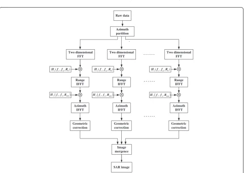
Based on the above analysis, the full algorithm flow chart is shown in Figure 2.
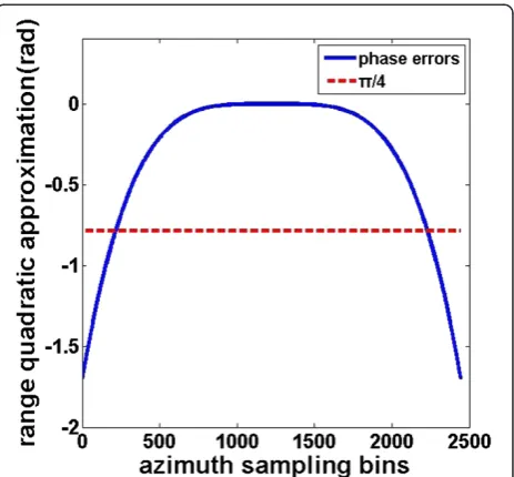
Figure 3Phase errors for quadratic range approximation.
Theoretically, the proposed algorithm can process the data over the full rotation. But in practice, we prefer to divide the data into several parts to alleviate the pressure of the computer memory. There are certain overlaps be-tween two divided block echo data just like the conven-tional stripmap data processing. It is necessary to clarify that the divided block data should include a whole inte-gration time of the interested target, namely, the interval from the beginning to the end of the illumination of the target. These procedures about azimuth data segmenta-tion, geometric correcsegmenta-tion, and image mergence are simi-lar to the relative operations represented in [16], readers can refer to them.
The detailed steps to complete imaging are given as follows:
Step 1 Segment the data into blocks in azimuth. Step 2 2D FFT to transform the echo signal presented in (5) to 2D frequency domain as shown in (15). Step 3 Compensate the range migration termφrcm(fη),
range modulation termφrg(fη), residue phase termφres
(fη,fτ), and SRC termφsrc(fη), this can be implemented
by multiplying them with their conjugate phase,
H1 fτ;fη;R0
Step 4 Range IFFT to convert the signal to the range Doppler domain and then multiply it with the azimuth match filtering function to finish azimuth compression. The azimuth match filtering function is presented as follows:
Step 5 Perform azimuth IFFT to obtain a well-focused SAR image for each block.
Step 6 Merge all the block sub-images into a whole image after operating geometric correction.
3.4. Theoretical resolution
For CTSSAR, the analytical expression of range theoret-ical resolution is the same as that of the conventional rectilinear stripmap SAR, namely, ρr¼ c
2B, where B is the bandwidth. However, due to the impact of the circu-lar trajectory, the azimuth theoretical resolution is dif-ferent from that in the conventional stripmap mode. Assuming that there are two point targets with azimuth angle difference Δθ, the Doppler difference of the two targets can be expressed in the following equation based on the range equation (1).
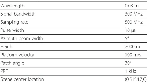
Table 1 Radar parameters
Wavelength 0.03 m
Signal bandwidth 300 MHz
Sampling rate 500 MHz
Pulse width 10μs
Azimuth beam width 5°
Height 2000 m
Platform velocity 100 m/s
Patch angle 30°
PRF 1 kHz
Scene center location (0,5154.7,0)
Δf ¼2ωrλarpsinΔθ Rcen
ð26Þ
Let the azimuth integration time beTdand the number of it N. We suppose that the interval of the two selected point targets is the system minimum distinguishable unit. Then
fPRF
N ¼
2ωrarpΔθ
λRcen ;
ð27Þ
where fPRF denotes the pulse repetition frequency. From (27), the analytical expression for the azimuth theoretical resolution in CTSSAR can be obtained.
ρa¼rpΔθ¼λRcenfPRF 2Nωra
¼λRcen
2vTd
ð28Þ
Here, we use the expression of Doppler FM rate for CTSSAR.
ka ¼ 2vvp
λRcen
ð29Þ
Hence, the expression of azimuth theoretical reso-lution is obtained, that is, ρa¼λRcen
2vTd . In addition,
relational analysis can be found in [16] and readers can refer to it.
4. Simulation results
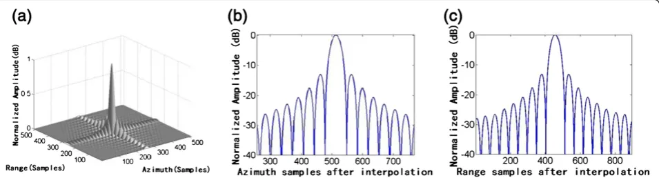
In SAR imaging, the negligible high-order term error should satisfy the criterion that the maximum double range phase error is less than π/4 rad for the range ap-proximation errors [19]. Herein, it is necessary to select an appropriate approximated order. On one side, if the approximation order is too small, the precision will not be large enough to focus the image data. On the other side, too large an approximation order will surely bring certain extra computation, but it will not be the main computational consumption in the practical use for the reason that it is too small compared with the primary computational operation and it can be precalculated and set in the RAM. Nevertheless, more important is that if higher-order range approximation is adopted, the deriv-ation of the 2D spectrum will become very complex and difficult when using MSR [17], especially for the case that the order is larger than fourth-order, the condition under which it is very complicated for calculating the 2D spectrum. In addition, it is widely accepted that the com-putational complexity of the time domain BP algorithm is Figure 6Center point imaging result using the proposed method.(a) 2D impulse response. (b) Azimuth impulse response. (c) Range impulse response.
O(N3) [15]. Taking the complex multiplication into con-sideration, as illustrated in [19], the number of floating point operations (FLOPs) is used here to estimate the computation load of the algorithm. An FFT or IFFT of length N requires 5 N log2(N)FLOPs. A complex phase multiplication requires six FLOPs. It is assumed thatNais the number of input lines (azimuth samples); Nr is the number of input range samples per line. Thus, according to the algorithm flowchart, there are four FFT (or IFFT) operations and two complex multiplication operations:
Ntotal¼5NrNalog2ð Þ Nr 3þ6NrNa2
þ5NrNalog2ð ÞNa ð30Þ
Therefore, letNr=Na=N, the computational complex-ity of our algorithm is O(N2log2(N)), which is a tremen-dous improvement for the computational efficiency. In the following simulation, corresponding computational pro-cessing time experiments will be carried out with related analyses. Now let us discuss how large the order is needed to satisfy the request of imaging quality.
Here, we choose a series of typical parameters. As-sume that the parameters of the flight platform are
Hc = 2000 m,ra= 4000 m, rp= 5154.7 m,v= 100 m/s, and the wavelengthλ = 0.03 m, now compute the quad-ratic approximation errors and the quartic approximation errors in one synthetic aperture, as shown in Figures 3 and 4, respectively. The dashed line denotes the location when the phase error is π/4 rad, and the solid line indi-cates the phase errors introduced by different range approximations in the integrated synthetic aperture time.
Besides, the cubic approximation errors are not consid-ered here for the fact that the odd terms are all zero. It can be seen clearly from the figure that the maximum value of the quadratic approximation errors is about 1.7 rad, larger thanπ/4 rad indicated by the dashed line in the figure, which implies that the approximated errors intro-duced by quadratic approximation cannot be ignored, or the degradation of the image focusing may occur. How-ever, the maximum quadratic approximated errors is about 3 × 10⁻³ rad, far less thanπ/4 rad, so the dashed line does not noted in the figure. Thus, it is obvious that the expression in (15) is more applicable than the quad-ratic approximated one.
In order to verify the effectiveness of the proposed algorithm in this article, let us compare our algorithm with the quadratic approximation method in terms of image quality. The simulation parameters are shown in Table 1, there are three target points Pn, Pm, and Pf in the scene, and their coordinates arePn(0, 4854.7, 0),Pm (0, 5154.7, 0), andPf(0, 5454.7, 0), respectively.
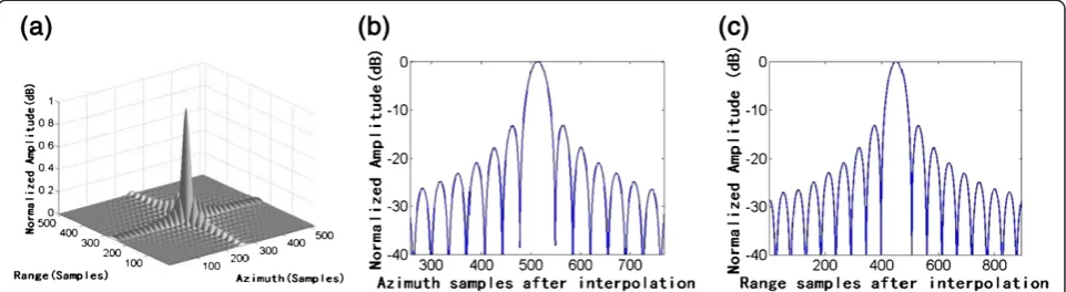
The imaging results of the two algorithms for the same scene center point is shown in Figures 5 and 6 to com-pare the two algorithms, where (a) is the 2D impulse re-sponse of the target point, (b) is the azimuth impulse response, and (c) is the range impulse response. From the figure, we can see that the quadratic approximation is not able to represent the enough phase variant infor-mation and the focusing is not satisfied. In contrast, the algorithm proposed in this article keeps the range up to fourth-order and presents more range-variant informa-tion in the 2D frequency domain. So, it is possible to Figure 8Farthest point imaging result using the proposed method.(a) 2D impulse response. (b) Azimuth impulse response. (c) Range impulse response.
Table 2 Image quality parameters using the proposed method
Parameter Theoretical one Pn Pm Pf
Azimuth Range Azimuth Range Azimuth Range Azimuth Range
Resolution (m) 0.125 0.443 0.126 0.443 0.126 0.445 0.126 0.443
PSLR (dB) −13.26 −13.22 −13.29 −13.25 −13.26 −13.69 −13.28
have access to the accurate image with high resolution. Figures 7 and 8 are the imaging results of the nearest point and the farthest point using our method, respect-ively. It is obvious that not only the center point, but also other points in different range are all well focused, which prove the feasibility of the proposed method successfully.
Table 2 lists the image quality parameters to the three points of our algorithm. Besides, the theoretical range resolution and azimuth resolution are 0.443 and 0.125 m, respectively [16]. It can be seen from Table 2 that each parameter is close to the theoretical one, which in-dicates satisfactory imaging results and further validates the effectiveness and feasibility.
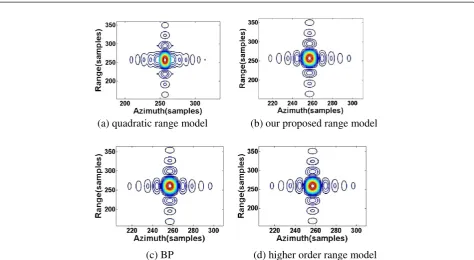
To further illustrate the superiority of the proposed algorithm over other imaging methods, some imaging results are provided and computational experiments are implemented here. Figure 9 indicates the contour plots of different imaging method for a selected point target
Pm, where Figure 9a delineates the imaging result for the quadratic range approximated algorithm, Figure 9b shows the contour of the proposed algorithm based on quartic range approximation, Figure 9c represents the result of BP algorithm, and Figure 9d is the image for higher-order range approximation (sixth-order is used here). It is obvious that the quadratic approximation is not precise enough to focus the image in CTSSAR and the time domain BP algorithm seems to be trusted to
(a) quadratic range model
(b) our proposed range model
(c) BP
(d) higher order range model
Figure 9Comparison of different imaging method for a selected point target.(a) Quadratic range model. (b) Our proposed range model. (c) BP. (d) Higher-order range model.
H (m)
Phase errors(rad)
-1 -0.5 0 0.5 1 -400
-200 0 200 400
a r Δ
Phase errors(rad)
-1 -0.5 0 0.5 1 -300
-200 -100 0 100 200 300
-2 -1 0 1 2
-15 -10 -5 0 5 10 15
ω
Δ (rad/s)
Phase errors(rad)
(a) height
(b) radius (c) angle velocity
(m)
handle this task perfectly. Unfortunately, too huge the computational load makes it difficult to be applied to the practical engineering use. In contrast, our proposed method can have an access to an ideal result with high computational efficiency. In addition, we can find that the image with higher-order approximation is well fo-cused as well, but we can hardly find any improvement over Figure 9b. So, it confirms that our approximation accuracy is high enough and an extra higher-order ap-proximation appears to be unnecessary in CTSSAR pro-cessing. Besides, the higher the approximated order is, the harder the derivation of the 2D spectrum is.
In order to validate the computational efficiency of our algorithm, the computational loads are measured. In our practical experiment, the operation time for the time domain BP algorithm is 14676.80 s, the time for our proposed algorithm is 40.43 s, and the higher-order approximation method (we use sixth-order approxima-tion to simulate here) consumes 48.58 s. Although the quadratic method needs only 26.67 s, we can see obvi-ous defocused phenomenon in the obtained image (shown in Figure 9a). So, we can easily get a conclusion that the BP algorithm is too slow for imaging, the quad-ratic method cannot reach our imaging standard, and the higher-order method needs a little more time com-pared with the proposed method (though we can optimize the procedure in the practical use as mentioned before) without any improvement for the imaging. Moreover, the higher-order approximation will bring huge calculating obstacles for the derivation of the 2D spectrum using the MSR. Therefore, after comparison with all kinds of im-aging method, it is apparent that the proposed algorithm is a rational, wise choice for CTSSAR.
In practice, the platform cannot always move along an ideal circular path. The trajectory is influenced by many factors. And the sensitivity to the motion errors is ana-lyzed in the following. Three variables of the platform, namely, the heightHc, the flying radiusra, and the angle velocityω, are selected to carry out the experiment. The simulation experiment results are denoted in Figure 10, indicating the phase errors varying with each parameter errors. In addition, in SAR imaging processing, the max-imum phase error for range that will not result in defocus of the image is π/4 rad [19]. It can be seen from the figures that the phase errors are relatively susceptible to the variations of the parameters. The noticeable degrad-ation will take place when the radius error Δra ≥ 3.75 × 10⁻³m, the height errorΔh≥2.165 × 10⁻³m, or the angle velocity error Δω ≥ 0.1346 rad/m. Thus, to compensate for these motion errors, the platform should be equipped with a global positioning system and high accurate inertial navigation system (INS), and more autofocusing tech-niques are required to be introduced to accomplish fine motion compensation lest the case that the INS cannot
meet the request of the motion compensation. Further-more, if the moving path is too far away from ideal and the trajectory is too complex to make the frequency-domain algorithm being available, the time-frequency-domain algo-rithm (such as BP method) may be an excellent choice.
5. Conclusions
In this article, the CTSSAR imaging geometry model is established first, and the imaging difficulties and obstacles are unveiled. Then the point target range function and its 2D frequency spectrum are deduced by MSR, the problem of choosing the approximation order is solved through the analysis of the approximated phase errors and it is verified by related experiments. Based on the derived spectrum, the corresponding modified Omega-K method is devel-oped. The high-order term introduced from the circular track is compensated at the beginning of the algorithm. Range compression and RCMC are then conducted in 2D domain followed with azimuth compression to obtain a sub-image, the ultimate image is formed by merging all the sub-images together. Compared with the quadratic approximation method, the proposed method has more accuracy. At the end of the article, the feasibility and effi-ciency of the proposed approach are validated with the simulation experiments.
Competing interests
The authors declare that they have no competing interests.
Acknowledgments
The authors would like to thank the anonymous reviewers for their careful reading of this article and for their detailed and constructive comments that have improved the presentation of this article. This study was supported in part by the National Natural Science Foundation of China under grant 61222108 and in part by the“973”program of China under grant 2010CB731903.
Received: 28 June 2012 Accepted: 4 March 2013 Published: 28 March 2013
References
1. RK Raney, H Runge, R Bamler, IG Cumming, FH Wong, Precision SAR processing using chirp scaling. IEEE Trans. Geosci. Remote Sens.
32, 786–799 (1994)
2. N Gebert, G Krieger, Azimuth phase center adaptation on transmit for high-resolution wide-swath SAR imaging. IEEE Geosci. Remote Sens. Lett.
6, 782–786 (2009)
3. C Cafforio, C Prati, F Rocca, SAR data focusing using seismic migration techniques. IEEE Trans. Aeorsp. Electron. Syst.27, 194–207 (1991) 4. M Soumekh,Synthetic Aperture Radar Signal Processing With Matlab
Algorithms(Wiley, New York, 1999)
5. K Knaell, Three-dimensional SAR from curvilinear apertures. Proceedings of IEEE Radar Conference, Carderock Div2230, 220–225 (1996). NSWC, Bethesda, MD, USA
6. D Falconer, G Moussally, Tomographic imaging of radar data gathered on a circular flight path about a three-dimensional target zone. Proceedings of SPIE, Aerosp, Syrup2487:2–12 (1995). Orlando, FL
7. A Ishimaru, T Chan, Y Kuga, An imaging technique using confocal circular synthetic aperture radar. IEEE Trans. Geosci. Remote Sens.36, 1524–1530 (1998) 8. M Bara, L Sagues, F Paniahua, A Broquetas, X Fabregas, High-speed focusing
algorithm for circular synthetic aperture radar. Electron. Lett.
9. H Cantalloube, EC Koeniquer,Airborne SAR imaging along a circular trajectory, in(Proceedings of EUSAR, Dresden, Germany, 2006), pp. 16–19 10. H Cantalloube, EC Koeniquer, H Oriot,High resolution SAR imaging along
circular trajectories(Proceedings of IGARSS, Spain, Barcelona, 2007), pp. 850–853
11. M Soumekh, Reconnaissance with slant plane circular SAR imaging. IEEE Trans. Image Process.5, 1252–1265 (1996)
12. M Ferrara, JA Jackson, C Austin, Enhancement of multi-pass 3D circular SAR images using sparse reconstruction techniques, in. Algorithms for Synthetic Aperture Radar Imagery XVI, Proceedings of SPIE7337, 733702 (2009). Orlando, FL
13. M Pinheiro, P Prats, R Scheiber, M Nannini, A Reigber, Tomographic 3D reconstruction from airborne circular SAR. Proceedings of IGARSS
3, III21–III24 (2009). Cape Town, South Africa
14. O Ponce, P Prats, MR Cassola, R Scheiber, A Reigber,Processing of circular SAR trajectories with fast factorized back-projection, in Proceedings of IGARSS
(Proceedings of IGARSS, Vancouver, Canada, 2011), pp. 3692–3695 15. Y Lin, W Hong, WX Tan, YR Wu, Extension of range migration algorithm to
squint circular SAR imaging. IEEE Geosci. Remote Sens. Lett.
8, 651–655 (2011)
16. B Sun, YQ Zhou, J Chen, CS Li, Operation mode of circular trace scanning SAR for wide observation. J. Electron. Inf. Technol.30, 2805–2808 (2008) 17. YL Neo, FH Wong, IG Cumming, A two-dimensional spectrum for bistatic
SAR processing using series reversion. IEEE Geosci. Remote Sens. Lett.
4, 93–96 (2007)
18. YL Neo, FH Wong, IG Cumming, Processing of azimuth-invariant bistatic SAR data using the range Doppler algorithm. IEEE Trans. Geosci. Remote Sens.46, 14–21 (2008)
19. IG Cumming, HW Frank,Digital Processing of Synthetic Aperture Radar Data: Algorithms and Implementation(Artech House, Norwood, MA, 2005)
doi:10.1186/1687-6180-2013-64
Cite this article as:Liaoet al.:A novel modified Omega-K algorithm for circular trajectory scanning SAR imaging using series reversion.EURASIP Journal on Advances in Signal Processing20132013:64.
Submit your manuscript to a
journal and benefi t from:
7Convenient online submission
7Rigorous peer review
7Immediate publication on acceptance
7Open access: articles freely available online
7High visibility within the fi eld
7Retaining the copyright to your article