R E S E A R C H
Open Access
Efficient compressive sampling of spatially
sparse fields in wireless sensor networks
Stefania Colonnese, Roberto Cusani, Stefano Rinauro
*, Giorgia Ruggiero and Gaetano Scarano
Abstract
Wireless sensor networks (WSNs), i.e., networks of autonomous, wireless sensing nodes spatially deployed over a geographical area, are often faced with acquisition of spatially sparse fields. In this paper, we present a novel bandwidth/energy-efficient compressive sampling (CS) scheme for the acquisition of spatially sparse fields in a WSN. The paper contribution is twofold. Firstly, we introduce a sparse, structured CS matrix and analytically show that it allows accurate reconstruction of bidimensional spatially sparse signals, such as those occurring in several surveillance application. Secondly, we analytically evaluate the energy and bandwidth consumption of our CS scheme when it is applied to data acquisition in a WSN. Numerical results demonstrate that our CS scheme achieves significant energy and bandwidth savings with respect to state-of-the-art approaches when employed for sensing a spatially sparse field by means of a WSN.
1 Introduction
Wireless sensor networks (WSN) consist of autonomous, cooperative sensors spatially deployed over a geographi-cal area, with applications ranging from surveillance [1] and localization systems [2,3], to environmental monitor-ing for physical field sensmonitor-ing and disaster prevention [4,5]. WSN nodes typically acquire the data and communicate them to a node named fusion center (FC), which stores the sensors’ readings or forwards them through wired network infrastructures for further processing.
The availability of energy-efficient algorithms for data gathering towards the FC is particularly relevant when the monitoring network is deployed on a large geograph-ical area (e.g., a forest), where highly efficient routing protocols are required for a sustainable network lifetime. Energy efficiency is also relevant in those environments where battery recharge or substitution may be unworkable (e.g., in underwater networks) [6,7]. On the other hand, efficient exploitation of available bandwidth is an impor-tant concern in bandwidth-limited or interference-limited environments.
The unifying sampling and compression approach of compressive sampling (CS) [8] is definitely well suited
*Correspondence: [email protected]
Dipartimento di Ingegneria dell’Informazione, Elettronica e delle
Telecomunicazioni (DIET), Università di Roma “La Sapienza”, Via Eudossiana 18, Rome 00184, Italy
to resource-limited WSNs’ applications. CS-based tech-niques for energy-efficient WSN data gathering have been recently investigated, with particular reference to the trade-off between reconstruction accuracy and data gath-ering cost [9]. A highly efficient approach is provided by random sensing (RS), where at each observation time, only a randomly drawn subset of sensors acquires data and transmits them to the FC, typically using single-hop links. From a theoretical point of view, RS and CS share conditions and procedures for signal reconstruction. An energy- and bandwidth-efficient RS procedure appears in [10].
WSN monitoring applications are often faced with acquisition of spatially sparse signals. A typical example is that of temperature-monitoring sensor networks for anomalous event (e.g., fire) detection: in the early stages of abnormal system behavior, in which the event is hopefully detected, the field is characterized by one or more small spots at levels largely different from the surroundings, and it can be modeled as a spatially sparse signal. RS schemes, such as those analyzed in [10], poorly perform in sampling signals that are naturally sparse in the spatial domain since the actual number of measurements required to recon-struct the field increases and the RS bandwidth/energy efficiency deteriorates.
This paper successfully addresses the efficient compres-sive sampling of spatially sparse signals in a WSN. We introduce a novel CS scheme that can be realized in a
WSN by distributed and parallel data gathering schemes, with restrained energy and bandwidth consumption for inter-sensor signaling. Specifically, the main contributions of this work are the following:
• We introduce a novel CS matrix and analytically demonstrate that it satisfies the CS conditions for sparse signal reconstruction.
• We analytically evaluate the performance, in terms of energy and bandwidth efficiency, of a WSN data gathering scheme based on the CS matrix presented herein.
• We show that, on spatially sparse fields, our CS scheme outperforms selected RS and CS
state-of-the-art ones in terms of both energy and bandwidth efficiency.
The remainder of the paper is organized as follows: Section 2 describes the WSN system model, Section 3 briefs the CS basics, and Section 4 discusses related works on CS/RS acquisition in WSN. In Section 5 we illustrate our original CS scheme, and in Section 6 we apply it to a WSN and analyze the related energy consumption and bandwidth occupancy. Section 7 presents numeri-cal results assessing that our CS scheme outperforms state-of-the-art approaches in terms of bandwidth/energy efficiency. Section 8 concludes the paper.
2 System model and network scenario
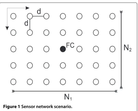
Let us consider a physical field represented by a bidimen-sional time-varying signals(x,y;t),(x,y)∈R2monitored through a grid of N = N1× N2 sensors deployed over a bidimensional covered area,N1andN2being the num-ber of sensors distributed in the horizontal and vertical dimension, respectively. A selected sensor collects the data from the others and plays the role of FC. An exam-ple of such a WSN scenario is depicted in Figure 1: the FC is placed at the center of the network, and each sen-sor is placed at distance dk,k = 1,. . .,N − 1 from the FC.
The sensors periodically measure s(x,y;t) and trans-mit their readings to the FC for monitoring. The sensing period t is selected to be almost equal to the coher-ence time Tc of s(x,y;t)a. At time tk = t0 + kt, the sensor at the location (n1d,n2d) acquires the noisy measurement:
z[n1,n2]=s(n1d,n2d;tk) (1)
where, for the sake of simplicity, we have dropped the temporal variable and have set the horizontal and verti-cal inter-sensor distances equal to d. Then, the sensors implement a suitable dissemination protocol to forward the measured value to the FC. The FC collects all the data
Figure 1Sensor network scenario.
from the sensors so as to reconstruct a representation of the overall fieldz[n1,n2].
Efficient data dissemination towards the FC is widely debated in the literature since energy efficiency affects the network lifetime, especially relevant in scenarios where the deployment of sensors is difficult or expensive, whereas bandwidth efficiency enables WSN monitoring in bandwidth-limited media, e.g., underwater, or in geo-graphical areas where different sensor networks coexist. CS and RS paradigms provide a theoretical framework for highly efficient field monitoring, provided that the mon-itored data are sparse in a suitable domain. We briefly recall in Sections 3 and 4 the basics of CS and the related work on CS and RS application in WSN, respectively.
3 An introduction to compressive sampling
Let us compactly represent the bidimensional sequence z[n1,n2] by the lexicographically ordered vectorz:
z=[z[1, 1]· · ·z[1,N2] z[2, 1]· · ·z[N1,N2]]T. The vectorz ∈ RN is sparse if the number of its non-zero samples is restrained compared to its own dimension N; rigorously, zis said to be K-sparse if the number of non-zero components is K, either in the spatial or in a transformed domain (e.g., Fourier, wavelet, etc.). CS pro-vides a framework for sensing and compression of a sparse signal.
According to the CS paradigm, compression of sparse signals is performed jointly with the acquisition. Specifi-cally,zis represented byMprojections defined as follows:
y=z (2)
be accurately recovered from the projections inyprovided thatK<M<N. Specifically, the sensing matrixmust satisfy the so-called restricted isometry property (RIP), i.e., given a constantδ, for allK-sparse signalsz, it must stand:
(1−δ)||z||22≤ ||z||22≤(1+δ)||z||22.
It is proven [11] that, for values ofδsmall enough, sparse signals can be perfectly recovered from compressive sens-ing measurements. In [12], the authors show that the RIP property is verified when the measurement energy||z||2 is more and more concentrated, in probability, around the value ||z||22 as far as the number of measurements increases.
Reconstruction can be achieved either by solving the following optimization problem:
ˆ
z=arg min
t ||t||1 s.t. y=z (3)
or by a greedy iterative pursuit of the support ofz; exam-ples of this latter approach are provided by the orthogo-nal matching pursuit [13] and the compressive sampling matching (CoSaMP) algorithms [14].
In (2), we recognize that randomly sampling the com-ponents of z and collecting them in y is equivalent to realizing CS using a particular sensing matrix; therefore, many CS theory results apply to RS, too. Both RS and CS techniques have been considered for application in WSNs.
4 Related works
Efficient sensing and data gathering in WSNs by means of CS- and RS-based techniques have aroused lively inter-est in recent literature. In [15], a CS-based distributed communication architecture is exploited to minimize the latency for information retrieval under a favorable power-distortion trade-off, whereas in [16], a CS-based sensing and data gathering procedure is analyzed for the case of network routing tree topologies. In [17], maximiza-tion of large-scale WSN lifetime is pursued by means of a fully distributed algorithm according to which each sensor autonomously performs classical or compressive sampling in order to reduce the number of transmitted packets.
In [9], the authors analyze a RS and multi-hop data gathering scheme. In this scheme, only randomly selected nodes measure the field and transmit their readings to the FC through specific multi-hop paths. While a sensor reading is routed towards the FC, its value is combined
with the ones sensed by the sensors in the path, so that each random projection provided to the FC is built by accumulating randomly weighted sensor read-ings along a network path. Energy efficiency is pursued if the number of nodes contributing to each projection is low.
In [18], a peculiar form of the CS sensing matrix is proven to exhibit good reconstruction properties while still being able to reduce the number of inter-sensor trans-missions. The structure of the sensing matrix, originally designed for WSNs with chain topology, is viable of an extension to more complex scenarios, provided that suit-ably tree-structured routing paths are designed from the exterior of the network towards the FC.
Recently, in [10] a RS-based sensor network frame-work for underwater systems has been introduced. Dif-ferently from the works in [9,16,17], a single-hop network is considered, where the sensors directly communicate
with the FC. Every sampling interval t, each
sen-sor senses the field and transmits it directly to the FC with probability p. The sensing probability p is suit-ably chosen in order to let the FC acquire sufficiently many data for field reconstruction. The approach in [10] favorably merges the RS procedure with a random access protocol, thus obtaining a significant reduction in both the consumed energy and the occupied band-width. The main reasons why the above discussed meth-ods achieve significant performances in efficient use of network resources are either in the fact that, during a sampling interval, only a subset of the sensors mea-sures the field by means of RS or in the fact that CS acquisition is actually realized jointly with the routing procedure.
Recent studies [16,18] suggest that in the case of spa-tially sparse signals, the energy/bandwidth of RS and CS efficiency deteriorates since reconstruction accuracy is guaranteed only when a large number of sensors contribute to the measurements. In [16], the authors remark how difficult it is to design a RS matrix suited to sparse signals and still allowing an efficient network routing. In [18], it is pointed out that, on spatially sparse signals, CS techniques still guarantee reconstruc-tion accuracy but at an increased number of measure-ments (e.g., M up to 50% of N), whereas for the same values of M and N, RS only opportunistically achieves reconstruction.
clusterization is selected depending on the sparsifying basis under which the field is sensed. The clusteriza-tion corresponds to a sparse structure in the sensing matrix, and it is the starting point to allow energy savings in the overall sensing procedure, realized by a central-ized algorithm. The procedure is designed for spatially localized signals, which are sparse in a spatially localized basis (e.g., Daubechies, DCT), but it looses efficiency as the signals become more and more sparse in the spatial domain.
On the other hand, in several WSN applications, the sensed field indeed contains local fluctuations and abnor-mal readings, and it is well modeled as a spatially sparse signal. This motivated us to concern ourselves with the design of a sensing matrix suited to spatially sparse sig-nals, as described in the following section.
5 CS using Radon-like random projections
In a nutshell, we aim at devising a sensing matrix that represents a spatially sparse field z in a domain such that dropping N−Mcomponents does not prevent sig-nal reconstruction. Recalling that the Radon transform has the dual properties of (1) compressing spatial domain straight lines into transform domain pulses [20] and (2) expanding spatial discrete pulses into as many non-zero values as the number of considered Radon projections [21], we recognize that the Radon transform provides a mean for redundant representation of sparse signals built by spatially isolated pulses. Thereby, we resort to a spa-tially sparse signal CS scheme inspired by the Radon projection computation.
To elaborate, let us consider the bidimensional sequence z[n1,n2] of finite size N1 ×N2, and let us present few examples of measurements computed in analogy to the Radon projections. First, let us consider the column-wise accumulation of a randomly weighted version of z[n1,n2]:
y(0)[m]= N2−1
i=0
ϕ(m0)[i]z[i,m] , m=0,. . .,N1−1 (4)
where ϕm(0)[i] ,i = 0,. . .N1 − 1,m = 0,. . .,N2 − 1 are independent and identically distributed (i.i.d.) zero mean Gaussian random variables of equal variance σϕ2, i.e., ϕm(0)[i]∼ N(0,σϕ2); an example of the formation of
the measurements y(0)[m] is illustrated in Figure 2. The measurements y(0)[m] differ from a Radon projection in that each sample is randomly weighted. Besides, they dif-fer from classical CS measurements in that each measure is obtained only from a subset (namely a column) of the values in z[n1,n2] rather than from all the samples z[n1,n2].
n
1n
2z
[
n
1,n
2]
y
(0)[
m
]
Figure 2Bidimensional sequencez[n1,n2]: column-wise
accumulation for computation of the measurementsy(0)[m].
Definition of the row-wise random projections of z[n1,n2] is straightforward, namely:
y(π/2)[m]= N1−1
i=0
ϕm(π/2)[i]·z[m,i] , m=0,. . .,N2−1.
(5)
By analogy, we can define the diagonal-wise projection ofz[n1,n2] as well:
y(π/4)[m]= ⎧ ⎪ ⎪ ⎪ ⎪ ⎪ ⎪ ⎪ ⎨ ⎪ ⎪ ⎪ ⎪ ⎪ ⎪ ⎪ ⎩
N1−1−m
i=0
ϕ(π/m 4)[i]z[i+m,i] ,
m=0, . . .,N1−1 N2−1−|m|
i=0
ϕm(π/4)[i]z[i,i+m] ,
m= −N2+1,. . .,−1. (6)
Expressions (4) to (6) represent randomly weighted accumulations of z[n1,n2] over ridge paths. Let us now generalize the above expressions by regarding them as obtained by column-wise accumulation of a suitably rotated version of the sequencez[n1,n2].
Letz(ϑp)[n1,n2] be aϑ
p-radiant clockwise-rotatedb ver-sion of the imagez[n1,n2]. The size ofz(ϑp)[n1,n2] varies with ϑp, and we denote as K(p),p = 0,. . .P − 1 the number of columns of z(ϑp)[n1,n2]. We generalize def-initions (4) to (6) by considering the collection of the random projections ofz(ϑp)[n
y(ϑp)[m]= i
ϕ(ϑmp)[i]·z(ϑp)[i,m] (7)
for m = 0,. . .K(p) − 1, p = 0,. . .P − 1. Since the accumulation in (7) recalls the column-wise accumula-tions employed in the computation of the discrete Radon transform, we refer to the projections in (7) asRadon-like random projections.
Let us now collect thePRadon-like random projections:
y(ϑp)=y(ϑp)[0]· · ·y(ϑp)[K(p)−1] T,p=0,. . .P−1
in a measurement vectory:
y=[y(ϑ0)T· · ·y(ϑP−1)T]T.
The measurementsyare computed fromzas
y=Rz (8)
using thepK(p)×N1N2random sampling matrixR defined as
where (ϑRp),p = 0,. . .P − 1 are the suitably defined sparse random matrix realizing the accumulation in (5) and (6). Specifically, the matrices(ϑRp),p = 0,. . .P−1 are built as follows. For each and every row, a few ele-ments, corresponding to the coefficients ofxthat do not contribute to the measurement, are deterministically set to zero. The remaining non-zero elements are drawn from i.i.d. normal distribution. For the sake of clarity, we report the matrices (R0) and (π/R 2), corresponding to the horizontal and the vertical projection, in (10) and (9), respectively.
Let us remark that, even though the samples contributing to each ycomponent are the same as those that would have contributed to a specific Radon projection ofz, due to the random weighting, the measurement vectoryis not - and it is not even easily related to - the Radon transform ofz.
In the following, we demonstrate that the conditions given by the CS theory for reconstructingzfromystand. Before turning to mathematics, let us observe that if the image z[n1,n2] is built by sparse isolated pulses, each pattern contributes, apart from a suitable random weight-ing, to each one of thePRadon-like random projections y(ϑp)[m] , m = 0,. . .K(p) − 1, p = 0,. . .P − 1. Thereby, the set ofPRadon-like random projections is a P-redundant representation of the pulse. This motivated us to formally demonstrate that the Radon-like random projectionsy(ϑp)[m] , m=0,. . .K(p)−1, p=0,. . .P−1 satisfy the conditions of a CS measurement set.
5.1 Restricted isometry property of the Radon-like
sampling matrix
To formally state that the above introduced simpli-fied sampling structure is feasible for accurate field reconstruction, we shall demonstrate that the random measurements y evaluated as in (8) are consistent CS measurements, i.e., they substantially preserve the infor-mation of the sampled sequencez[n1,n2].
Formally, we need to prove that the sampling matrixR satisfies the condition known as restricted isometry prop-erty. Specifically, let us denote byEzdef= ||z||2the quadratic norm of the vectorz. If the matrixRsatisfies
(1−δ)Ez≤ ||Rz||2≤(1+δ)Ez (11)
with high probability, then any sparse sequencezcan be perfectly recovered from CS measurementsy=Rz[11]. The RIP in (11) asserts that the measurement energy
Eydef= ||Rz||2 is strongly concentrated around the value Ez. Preliminary results on the RIP property of a Radon-like CS matrix appear in [22]. In Appendix 1, we extend these
(R0)= ⎡ ⎢ ⎢ ⎢ ⎢ ⎣
ϕ0(0)[0] 0 · · · 0 ϕ0(0)[N1−1] 0 · · · 0 0 ϕ0(0)[0] · · · 0 . . . . 0 ϕ0(0)[N1−1] · · · 0
0 ... . .. 0 0 ... . .. 0
0 0 · · · ϕN(0)
2−1[0] 0 0 · · · ϕ
(0)
0 [N1−1] ⎤ ⎥ ⎥ ⎥ ⎥
⎦ (9)
(π/R 2)= ⎡ ⎢ ⎢ ⎢ ⎣
ϕ0(π/2)[0] ϕ0(π/2)[1] · · · ϕ0(π/2)[N2−1] 0 0 · · · 0
0 0 · · · 0 . . . . 0 0 · · · 0
0 0 . . . 0 0 0 · · · 0
0 0 · · · 0 . . . ϕN(π/2)
1−1[0] ϕ
(π/2)
N1−1[1] · · · ϕ
(π/2)
N1−1[N2−1]
⎤ ⎥ ⎥ ⎥
results and, following the approach in [12], we show that the following property stands.
Property 1Let us assume that the entries in the matrix R are either deterministically set to zero, or i.i.d. zero mean Gaussian random variables with equal variance σϕ2 = 1/P. Then the following concentration inequality stands:
Pr{|Ey−Ez| ≥δ} ≤ (12)
provided that P ≥ 2K2C22log(2/ )/δ2,C2 being a suit-able constant. From Property 1, the RIP property in (11) immediately follows.
5.2 Further remarks
The sampling matrix R differs from the full sampling matrices usually adopted in CS since it is sparse. In the following, we show how the sparsity of the Radon-like sensing matrix R can be leveraged on to significantly simplify the CS measurement computation in a WSN so as to reduce the consumed energy and employed bandwidth. The definition ofy(ϑp)[m] in (7) given above is consistent and useful from an analytical point of view. When turn-ing to the evaluation ofy(ϑp)[m] in a WSN, the evaluation ofz(ϑp)[n
1,n2] is not accomplished, and the measurement computation is realized throughout the data gathering stage.
In [23], the authors demonstrate the RIP for a different kind of sensing matrix, that is, block diagonal matri-ces. With respect to the approach in [23], the proof in Appendix 1 is carried out asymptotically, that is, for M large enough to approximateEzas the outcome of a Gaus-sian random variables, and it leverages the hypothesis of a spatially sparse signal, i.e., a signal that is sparse in the canonical basis.
Finally, the concentration inequality (12) guarantees that the sequencezcan be recovered from the measure-mentsywith high probability, as far as the number Pof considered projections increases. Since CS convergence is assured only in probability, the CS measurement experi-ment could be repeated. In a WSN, data are periodically sensed and routed to the FC, and a small probability of mis-reconstruction can be tolerated since it can be recovered in the subsequent sampling interval. Further-more, integration of independently drawn measurements acquired in a WSN during different temporal intervals can be performed at the FC. This interesting research issue is deferred to further studies.
6 Radon-like CS in a WSN
In a WSN application scenario, thePRadon-like projec-tions correspond to randomly weighted sums of the values sensed by different subsets of WSN sensors. The sums can be evaluated using different techniques.
Following the approach in [24], the sensors within a subset can synchronously transmit their weighted sensed values, and the sum can be realized at the FC by on-air analogical superimposition of received signals. This pro-tocol requires strict control of the power received by the FC from each sensor. Precisely, each sensor node needs to estimate the channel seen towards the FC in order to pre-compensate the transmitted value according to the channel attenuation. Thereby, although feasible in princi-ple, this approach requires a sophisticated processing and tight power control by the sensor nodes.
According to a data gathering paradigm, the projections are computed within the network by a subset of sensors while they are forwarding their sensed values to the FC. The sums in (7) can then be realized by routing and accu-mulating values of z[n1,n2] over suitably tilted paths in the network grid discrete support.
Here we refer to such a data gathering approach, and we infer some consequences from the peculiar sparse struc-ture of the matrix R on the computation procedure. Firstly, we observe that in every row, the non-zero coef-ficients of the matrix R are arranged so as to obtain y(ϑp)[m] as the sum of the values of a column of the rotated imagez(ϑp). When collecting the measurement in a WSN, each projectiony(ϑp)[m] can then be computed by accu-mulating measurements throughout a specific, suitably tilted, grid path. Secondly, we observe that in every col-umn of the matrixR, there are onlyP non-zero values. Hence, each valuez[i,j] shall contribute only toPout of Mprojectionsy(ϑp)[m]. When realizing the Radon-like CS in the sensor network grid, each sensor shall transmit its valuePtimes.
Based on these premises, we recognize that the sparse structure of the matrixRresults into two main features of Radon-like projection computation in a WSN:
• The computation of each projectiony(ϑp)[m]is performed in a distributed way within the WSN, and it requires signaling among grid sensors which are adjacent along a WSN path.
• The accumulation along different paths can then be realized in parallel, provided that the distance between contemporaneously signaling nodes is kept large enough.
Figure 3Example of quadrant-based data gathering geometry for Radon-like CS measurements computation in a WSN.
following, this quadrant-based approach may be used to derive a specific data gathering procedure.
We now turn to quantifying the energy consump-tion and bandwidth occupancy required for realizing the Radon-like CS by means of a data gathering procedure in a WSN. In Section 6.1, we evaluate the energy con-sumption and bandwidth occupancy of the Radon-like CS scheme in a WSN. Next, we compare these results with selected state-of-the-art schemes, namely those of the random sensing approaches described in Section 1, detailed in Section 6.2.
6.1 Radon-like CS efficiency
We now evaluate the allocated bandwidth and consumed energy for entirely collecting the measurements in a time Tc in the WSN scenario in Section 2. The actual band-width occupation and energy consumption depend not only on the WSN structure but also on the adopted data gathering procedure. Without loss of generality, we refer to the suboptimal data gathering algorithm sketched out in Appendix 2, here briefly summarized for the reader’s convenience.
According to the algorithm in Appendix 2, the sen-sors transmit their readings to the FC by data gathering through suitable multi-hop paths. Figures 4 and 5 illus-trate, as an example, the multi-hop paths selected for the computation of the projectionsy(π/2)[m] ,y(π/4)[m] within
a network quadrant.
A deterministic (collision-free) time division multiple access (TDMA) is adopted. Signaling takes place between adjacent nodes only. Parallel transmission of nodes suffi-ciently apart is considered. In Appendix 2, we evaluate two parameters that directly affect the energy and bandwidth consumption of the data gathering algorithm, namely the total number of single-hop transmissions (NTX) and the
Figure 4Data gathering algorithm: spatial organization of sensors’ transmissions for horizontal projection evaluation in the first quadrant.Time stamps indicate when the node starts transmitting.
total number of time slots (NTS) needed to collect all the sensors’ readings to the FC.
The total number of node transmission, NTX, for the algorithm under concern comes out to vary linearly with the network size:
NTX≈γP·N, (13)
γP being a scalar factor depending on the adoptedP pro-jections. The guidelines for calculating γP are given in Appendix 2 where we also evaluate the value of γP for different sets of directionsϑp.
Based on the same data gathering algorithm, we have evaluated the number of time slots needed to collect all
the sensors’ readings to the FC. The number of time slots turns out to vary just with the square root of the network size, that is,
NTS≈δP· √
N, (14)
δP being a factor depending on the considered projec-tion direcprojec-tionsϑp. Appendix 2 reports the guidelines for the evaluation of the parameter δP for different sets of directionsϑp.
We observe that, as a consequence of the sparsity of the Radon-like sensing matrix, (1) the number of trans-mission varies only linearly with the network sizeN, and (2) the algorithm being parallelized, the number of time slots varies linearly with the square root of the network size N. With these results, we are able to evaluate the allocated bandwidth and consumed energy for entirely collecting the measurements in a time Tc in the WSN scenario described in Section 2.
Projection evaluation according to the data gathering scheme detailed in Appendix 2 accounts for a series of transmissions among neighboring nodes. The energy spent for a single-hop transmission is given by ESH = Gd2SHTp(RL), with dSH = d or
√
2d being the distance for horizontally, vertically, and diagonally adjacent nodes (a scale factor depending on the actual transmission parameters, namely the sensitivity at the FC receiver and the transmitter and receiver antenna gains) andTp(RL)the time needed for packet transmission.
Overall, we can express the total consumed energycfor the Radon-like CS-based approach as
ERL=NTXG d2Tp(RL). (15)
The packet durationTp(RL)depends on the design of the selected sensing system. If the overall sensing framework is designed under the system constraint of having a fixed occupied bandwidth B, the packet duration time will be evaluated asTp(RL)=L/BRLwithBRL=B.
This approach is suited to an application scenario where the bandwidth devoted to inter-sensor communications is fixed in advance. Other possible system constraints con-cern the time interval during which a whole set of mea-surement is acquired. In this case, the time for refreshing of the measurement is fixed to Tc. Stemming on such a design constraint, the packet duration time needed to assure that the measurements are collected within a max-imum time ofTcis written as follows:
Tp(RL)≤ Tc
NTS. (16)
Under this setting, the minimum occupied bandwidth, defined as the packet length in bits L over the packet
transmission time, for the Radon-like approach is evalu-ated as
BRL= L Tp(RL) ≥
L Tc
δP·√N. (17)
The relation providing the energy consumption in (15) can then be exploited either by considering an assigned packet time arising from a system bandwidth constraint or by assuming a given sensing rate 1/Tc. In the latter case, the packet duration is evaluated as in (16) so that the consumed energy reads as follows:
ERL= γP
δP
TcG d2· √
N. (18)
Such system design choices should be carefully taken into consideration when comparing energy consumption of different schemes possibly comprising different num-bers of single-hop transmissionsNTX.
When performing numerical simulations, we have con-sidered both the two aforementioned cases, namely:
• Fixed packet duration for the different compared schemes: this corresponds to a fixed system bandwidth constraint (cfr. results in Figure 6). • Fixed sensing procedure durationTc: this
corresponds to different packet durations (cfr. results in Figure 7).
6.2 RS efficiency
We now present a few results on the energy and band-width consumption of the approaches proposed in [10]. Therein, a RS procedure, allowing only a randomly chosen subset of sensors to acquire the measurement, is coupled with both a TDMA scheme and a random access scheme.
1000 1500 2000
Network Nodes
Consumed Energy
Consumed Energy
2500 3000 3500 400 1,0e+4
2,1e+5 4,1e+5
6,1e+5 RLRR RD
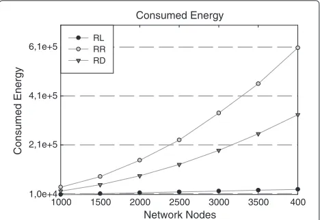
Figure 6Energy consumption versus number of nodesNunder the constraint of a fixed bandwidth occupancy.That is, the energy consumption for the different schemes is evaluated under the assumption of a fixed packet transmission time
0 1e+5 2e+5 3e+5
Figure 7Energy/bandwidth pairs.
Herein we elaborate on these results and add a few details. With respect to the computation in [10], where the energy consumption for each sensor to transmit to the network sink is approximated by a constant, here we explicitly take into account the dependence of the energy with respect to (w.r.t.) the spatial sensor location. Secondly, therein an approximate relation is established between two key system parameters, namely (1) the minimal fraction of sensing data that must be correctly received at the sink to allow CS reconstruction and (2) the minimal bandwidth. Herein we extend the relation to different ranges of sens-ing probability, better suited to RS of a spatially sparse field.
In the RS/deterministic access (RD) scheme, the FC ran-domly chooses a set ofMsensors, Mbeing a sufficient number of measurements for satisfactory field recon-structions and broadcasting the addresses of eliged nodes through the network. The selected nodes acquire the mea-surements and transmit their readings to the FC via a TDMA deterministic access scheme. As in this scheme onlyMnodes need to share the TDMA frame, the packet transmission time isTp(RD) = Tc/M. Consequently, the occupied bandwidth for the RD scheme isBRD=MTL
c. In order to evaluate the consumed energy, let us con-sider the setCM;Ncollecting all the possible configurations ofMout ofNnodes. The energy consumption of a given configuration c ∈ CM;N of M is expressed as E(c) =
p where the sum over the indexkcspans the Msensors within the combinationc. Thereby, the energy consumption of each combination depends on the dis-tances of theMnodes from the FC. In this respect, we evaluate the energy consumption of the RD scheme as the average over all the possible combinations: ERD =
1
cardinality ofCM;N. We recognize that in the overall sum over the KM;N combinations, the energy spent by each and every network sensor appears inMN−−11terms, cor-responding to the combinations it belongs to. Therefore, denotingN1def=α1
The energy consumption and occupied bandwidth perfor-mance of the scheme in [10] need to be addressed in a slightly different way w.r.t. the previous cases. CS theo-retic results determine the numberMof measurements needed at the FC to correctly restore the sensed field; within an observation time, this constraint corresponds to a required percentage qs of correctly received sam-ples at the FC. Because of possible collisions, the required percentageqsneeded at the FC does not translate straight-forwardly into a sensing probabilityps. In [10], the authors establish a relationship among the sensing probabilityps and the probability qs of correct packet reception and demonstrate that, given qs, a minimum bandwidthB is required in order to assure that a feasible value of ps exists. Thereby, if the available bandwidth is not accurately dimensioned, small values ofps do not provide enough measurements at the FC, whereas large values ofpscause too many collisions.
Besides, in [10], the authors provide an expression, standing for small values ofqs, of the minimum bandwidth as a function of the desiredqs. Following the guidelines in [10], we have extended such results to accommodate for large values ofqs, too. Specifically, we came up with the relationBminRR = TL The RS settings are therefore assigned as follows. Firstly, the desired qs is fixed according to the reconstruction quality constraints. Secondly, the minimum needed band-width is evaluated. Finally, the selected bandband-width value is employed to derive the needed sensing probabilityps[10]. With these positions, the packet transmission timeTp(RR) is determined from the employed bandwidth asTp(RR) = L/BminRR. Besides, the energy consumption is determined by the value ofps; the average network consumed energy is evaluated as
the powerN. The impact of these trends on energy con-sumption depends on all system parameters and mostly on ps. For a spatially sparse field, where ps and con-sequently qs tend to be high, since a large fraction of sensors shall transmit their values using RS with ran-dom access to allow proper reconstruction, a ranran-dom sensing scheme is prone to exhibit a large energy con-sumption and bandwidth occupancy. The Radon-like CS scheme then yields a reduced energy consumption for each node, as well as a parsimonious bandwidth use for collecting data over the entire grid. The gain is more and more evident as the network size (i.e., the covered area) increases.
Let us point out that, on non-spatially sparse fields, the conditions for accurate reconstruction, e.g., the values of ps andP, may differ, leading to different relative perfor-mances. The investigation of this issue is left for further studies.
The actual gain in terms of energy and bandwidth depends on the constants γP,δP which grow with the number of considered projections. The advantages of the Radon-like CS scheme are expected to be evident on spa-tially sparse signals, where low values of P (e.g.,P = 3) enable reconstruction, whereas the RS data gathering algorithm requires a high percentage of samples to reach the FC in order to achieve satisfying reconstruction results [18].
As far as the medium access scheme is concerned, the herein-devised Radon-like CS scheme is realized via a TDMA technique, just as the RD scheme. Therefore, it implies an effort of synchronization and scheduling. Nonetheless, different data gathering procedures can be envisaged realizing the Radon-like CS using a random access criterion. This issue is left for further studies. Finally, these results depend on the peculiar structure
of the Radon-like sensing matrix R and, although
derived for a particular data gathering algorithm, can be generalized to different Radon-like CS measurement computation schemes.
7 Numerical simulations
In this section, we analyze the performance of our Radon-like CS scheme both in terms of reconstruction accuracy and of employed network resources. Firstly, in Section 7.1 we present a few results showing that an accurate recon-struction of a spatially sparse signal can be achieved by the like CS using a feasible number of Radon-like projections. Secondly, in Section 7.2 we demonstrate the energy and bandwidth gain achievable when adopting the Radon-like CS scheme in a WSN. For fair compari-son of the different sensing techniques, we consider their performances under different system parameter settings, respectively corresponding to the case when each of the sensing system is operating at its minimal bandwidth and to the case of packet durationTpfixed for all the schemes. A comprehensive representation of the bandwidth-energy pairs of the different sensing systems is then shown ver-sus the network dimensionality. Finally, we present a few results assessing the performance of Radon-like CS sam-pling on real-world data.
7.1 Radon-like CS reconstruction accuracy
With reference to the network model in Section 2, we
consider a WSN made up by a square grid of N =
64 × 64 = 4, 096 sensors. The sensed field z[n1,n2] is built up by seven repetitions of an elementary 5× 5 pattern, differently scaled by factors in the range (0.5− 0.85]. Figure 8a describes an example of the fieldz[n1,n2]. This field adheres to the so-called pulse stream sig-nal model described in [25], and Algorithm 2 presented therein is employed for computing the reconstructed field
ˆ
z[n1,n2].
Figure 8Original fieldz[n1,n2](a) and reconstructed fieldzˆ[n1,n2](b) after sensing.Reconstruction was performed according to the
We have first evaluated the reconstruction accuracy of the Radon-like CS scheme, using different number P of projections, under the assumption of noise-free obser-vations. Specifically, we have tested the reconstruction accuracy when only projections along rows and columns of the network grid are considered (P = 2,M = 128), when projections along the rows, columns, and theπ/ 4-oriented diagonal of the grid are considered (P = 3, M = 255), and finally, also when projections along the 3π/4-oriented diagonal are considered (P = 4, M=382).
Table 1 reports the mean square error (MSE) of the reconstructed field zˆ, i.e., MSE = N1(z − ˆz)T(z − ˆz), achieved after 20 iterations of the reconstruction Algo-rithm 2 and averaged over ten runs corresponding to different pulse locations. Results in Table 1 show the effectiveness of the Radon-like CS scheme in sensing a sparse field with a restrained number of measurements. To visually assess the Radon-like CS scheme reconstruc-tion accuracy, we show in Figure 8b the reconstructed field
ˆ
z[n1,n2] obtained by measuring the field in Figure 8a with P=3 projections.
For the sake of comparison, we have also evaluated the reconstruction accuracy obtained by the RS [10] scheme under the same experimental settings. In Table 1 we recognize that, for the selected range of measure-ments(M ≤ 382), the RS does not allow capturing the sparse nature of the sensed field. To obtain the same reconstruction accuracy of the Radon-like CS scheme, namely a MSE equal to 0.0036, the RS requires to be
run with a number of measurements M 2, 500 ≈
50%N.
Similar results have been obtained by scaling the
num-ber of network nodes to N = 80× 80 = 6, 400 and
considering a sensed fieldz[n1,n2] composed by eight rep-etitions of the elementary pulse. The MSE of the Radon-like CS scheme, averaged over ten runs, is reported in Table 2. Also, in this case, the MSE obtained by the Radon-like CS scheme withP= {2, 3, 4}, corresponding toM=
{160, 319, 478}measurements, proves to exhibit satisfac-tory reconstruction quality. For the sake of comparison, we observe that in these experiments,M = 3, 500 were
Table 1 Reconstruction accuracy (MSE) obtained by Radon-like CS and RS schemes(N=64×64=4, 096)for different numbers of measurements
Parameter
M 128 255 382
P 2 3 4
ϑp 0,π/2 ϑp=0,π/2,π/4 ϑp=0,π/2,±π/4
Radon-like CS – MSE 0.0056 0.0019 0.0011
RS – MSE 13.3 7.604 4.721
Table 2 Reconstruction accuracy (MSE) obtained by Radon-like CS and RS schemes(N=80×80=6, 400)for different numbers of measurements
Parameter
M 160 319 478
P 2 3 4
ϑp 0,π/2 ϑp=0,π/2,π/4 ϑp=0,π/2,±π/4
Radon-like CS – MSE 0.0045 0.00152 0.000901
RS – MSE 8.602 6.472 4.506
needed by the RS to achieve analogous performance, namely a MSE equal to 0.006231.
Finally, we have tested the Radon-like reconstruction accuracy when noisy acquisition is considered so that the CS measurements can be modeled as
y=z+n
where the vectorngathers samples of white zero mean Gaussian noise with varianceσn2. In Table 3 we report the reconstruction accuracy obtained when acquiring with N =64×64=4, 096 sensors a field composed by seven patterns via the Radon-like CS scheme for different values ofσn2. Results in Table 3 show how the presence of noise in the acquisition process does not severely affect the recon-struction performance of the Radon-like CS approach.
To recap, the above results show that, as a rule of thumb, Radon-like CS requiresM≈P√Nmeasurements for rep-resenting a spatially sparse field, whereas the RS requires a large percentage of the measurementsMRS≈αNto be correctly received (e.g.,P = 3 andα =50% in the above experiments). Overall, the Radon-like CS scheme allows sensing and reconstructing of a spatially sparse field with far less measurement w.r.t. state-of-the-art techniques such as the RS presented in [10].
7.2 Radon-like CS efficiency
We now show that, besides using a restrained number of measurements, the Radon-like CS presents significant advantages in terms of energy and bandwidth needed to
Table 3 Reconstruction accuracy (MSE) obtained by the Radon-like CS, noisy measurements
(N=80×80=6, 400)
Parameter
M 128 255 382
P 2 3 4
ϑp 0,π/2 ϑp=0,π/2,π/4 ϑp=0,π/2,±π/4 Radon-like CS – MSE
forσn2=0.5
0.0065 0.0034 0.0033
Radon-like CS – MSE forσ2
n=0.7
disseminate sensor readings towards the FC. We evaluate the performance of Radon-like CS data gathering scheme (RL) by evaluating the consumed energy and occupied bandwidth under the following assumptions:
(a1) The number of measurements chosen is
large enough to yield a satisfactory reconstruction accuracy, quantified by a MSE≤10−3.
(a2) The coherence time of the sensed field is fixed to Tc=2, 500s.
(a3) The dimension of the transmitted packet is set to L=1Kb.
With reference to the experimental setting described in Section 7.1, condition (a1) implies P = 3 projections. We start by computing the energy consumption under the assumption that the occupied bandwidth and, conse-quently, the packet transmission timeTp = L/Bare the same for the different schemes.
Let us remark that, under this setting corresponding to a system design choice of having a fixed occupied bandwidth, each scheme requires a different number of transmissions in order to let the FC acquire the needed measurements. Thereby, the overall process of sensing is accomplished in different time intervals by the different data gathering techniques. In these experiments, we have set Tp(RL) = Tp(RD) = Tp(RR) = Tp = 0.61. Figure 6 reports the energy consumed for different numbers of network sensorsN. We recognize that employing the RL scheme drastically reduces the energy consumed by the data gathering algorithm.
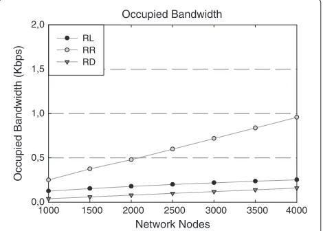
We then proceed to compute for the minimum occupied bandwidth required by the RL scheme to guarantee cor-rect sensing and reconstruction of a spatially sparse field under the constraint of a given refresh timeTc. Figure 9
1000 1500 2000 2500
Network Nodes
Occupied Bandwidth (Kbps)
Occupied Bandwidth
3000 3500 4000 0
1 2 3 4 5
RL RR RD
Figure 9Minimum bandwidth occupancy versus the number of nodesN.
plots the occupied bandwidth evaluated according to (17) versus the network size in terms of the number of sensors. For the sake of comparison, in the same figure, we also report the performance of RS, implemented using both a deterministic access scheme (RD in the legend) and the random access scheme (RR in the legend) described in [10]. The occupied bandwidth is computed according to the analysis in Section 6 for the RL, RD, and RR scheme, respectively, under the same assumptions (a1) to (a3). These settings imply ps = 0.5 for the RD scheme and qs=0.5 for the RR one.
The bandwidth employed for the Radon-like data gath-ering scheme is significantly reduced w.r.t. the RS, both using deterministic and random access. The above results, obtained by considering different numbers of measure-ments and equal reconstruction accuracy for the three algorithms, are explained by the efficiency of the Radon-like data collection algorithm, exploiting only single-hop, parallel data transmission.
We have then pushed further the comparison to find under which conditions the Radon-like and the RS schemes equally perform. In doing so, we have evalu-ated the bandwidth occupied by the RD and RR schemes when only 10% of the sensor readings are required to be correctly received by the FC. Figure 10 reports these results showing that the RL scheme still favorably com-pares with the RR scheme while requiring just slightly higher bandwidth w.r.t. the RD scheme. Therefore, the RL scheme overcomes the RD and RR ones unless they use a very low percentage of the sensors’ readings for field reconstruction.
Finally, we are interested in comparing the resource employed by the different schemes to accomplish the sensing process exactly at the same time. To reach this
1000 1500 2000
Network Nodes Occupied Bandwidth
Occupied Bandwidth (Kbps)
2500 3000 3500 4000 0,0
0,5 1,0 1,5 2,0
RL RR RD
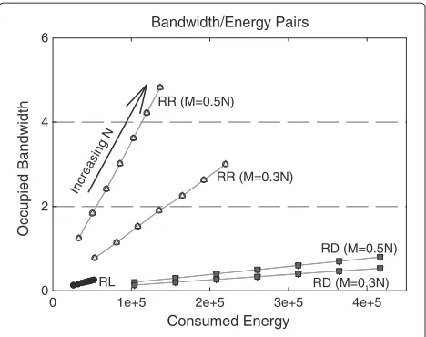
goal, as the number of single-hop transmissions varies from one scheme to another, the different schemes will have a different packet transmission time and hence will occupy a different bandwidth. In Figure 7, we illustrate the bandwidth-energy scatterplot of the RL, RR, and RD schemes for different network sizes. For RD and RR, we have considered two cases, that is, when 50% and 30% of the sensor readings are required at the FC for satisfactory field reconstruction.
The energy/bandwidth pairs draw different trajectories while the number of nodesN increases. We clearly rec-ognize a systematic energy and bandwidth saving of the RL scheme w.r.t. the competitors. Moreover, both the con-sumed energy and the occupied bandwidth exhibit far smaller variations with the number of network nodes than what happens with the RD and RR schemes, making the RL approach fully scalable in terms of network nodes.
7.3 Radon-like CS performances on real data sets
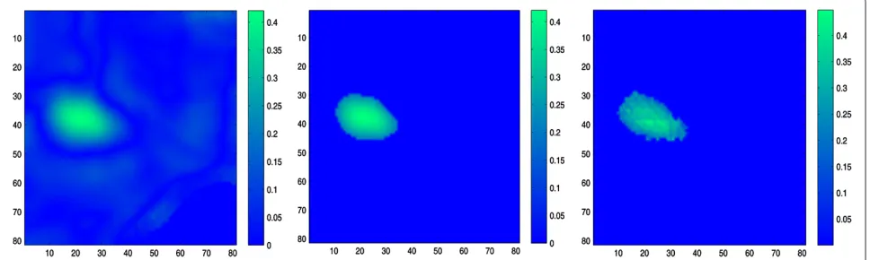
We now apply the Radon-like CS matrix to real-world data. Following the approach in [10], we resort to public oceanographic databases, namely the ones in [26]. Specif-ically, we have considered the compressive sensing acqui-sition of the ‘Zonal Current’ data at Monterey Bay on October 10, 2012. The Zonal Current data at the selected day are represented in Figure 11 (left). Let us highlight that the considered data are not spatially sparse. On the contrary, visual inspection of Figure 11 (left) shows how the field is represented by a pronounced pulse embed-ded in small values. Thereby, different approaches can be pursued. For instance, Radon-like sampling could be inte-grated with suitable basis transform to track for signal sparsity; this approach is left for further studies. Here we undertake a different procedure. Although the field is not strictly sparse as most of its values are indeed non-zero, we observe that it is yet true that most of the informa-tion conveyed by the field in Figure 11 (left) lies on its
peaks. For the reader’s convenience, we report in Figure 12 a histogram of the field values in Figure 11 (left), and in Figure 13, a histogram of the thresholded field value in Figure 11 (center) fort = 0.2. In Figure 12, we have also indicated the thresholding value (black dashed line) and the mean value of the sensed field (red solid line).
Stemming from this observation, we employ the Radon-like CS scheme to acquire a thresholded version of the original field. We acquire the(81×81) sensed field for different values of the threshold t, using a Radon-like scheme withP = 3. This scheme comprises projections along the rows, columns, and theπ/4-oriented diagonal of the grid, thus resulting inM = 323. Then we employ the CoSaMP algorithm as the reconstruction procedure. The reconstructed image is finally compared to the orig-inal, not thresholded, field so as to evaluate the MSE with respect to the original image. In Table 4, we report the results obtained for different values of the threshold t, corresponding to different degrees of sparsity of the thresholded image. We also report in Table 4 the number of non-zero samples in the thresholded image.
The results in Table 4 confirm the effectiveness of the Radon-like scheme in enabling reconstruction of the spa-tially sparse nature of the sensed thresholded field, achiev-ing MSE as low as 0.0036 for a high threshold value such as t = 0.2. As the thresholding factor, the number of non-zero coefficients in the thresholded image increases, making the Radon-like approach less effective. We would like to emphasize that application of Radon-like sensing matrices to non-sparse data could still be possible by tak-ing into account suitable sparsifytak-ing basis, which is left for further studies.
In Figure 11 (right), we report the reconstructed thresh-olded field after 15 iterations of the CoSaMP algorithm for t = 0.2; the corresponding original thresholded image is reported in Figure 11 (center). Visual inspec-tion of Figure 11 (right) shows how, in spite of the
0 0.05 0.1 0.15 0.2 0.25 0.3 0.35 0.4 0.45 0
100 200 300 400 500 600 700 800 900 1000
Figure 12Histogram of the sensed field values.The black dashed line represents the thresholding value, and the red solid line represents the mean value of the sensed field.
reduced number of measurements and of the restrained energy consumption, the Radon-like scheme is capable of capturing the spatially sparse nature of the recon-structed field. Finally, the approach outlined herein could be enforced by taking into account suitable padding of the data samples that are under the threshold, so as to substitute the zero entries obtained by the reconstruction algorithm with a specific non-zero value, e.g., their spatial mean, thereby reducing the observed MSE.
7.4 Final remarks
As a final remark, we observe that energy and band-width gain yielded by the Radon-like approach is directly based upon the favorable matching between the Radon-like matrix structure and the spatially sparse structure of the sensed field. Based on these results, we envisage a twofold extension of our work, namely:
0 0.05 0.1 0.15 0.2 0.25 0.3 0.35 0.4 0.45 0
100 200 300 400 500 600 700 800 900 1000
values
occurrences
Figure 13Histogram of the thresholded field values.The threshold has been set tot=0.2.
Table 4 Reconstruction performance in a real-data scenario (Zonal Current at Monterey Bay [26]) for different thresholding values
t S MSE against original MSE against
field thresholded field
0.1 826 0.003 0.0015
0.125 485 0.0031 8.20×10⁻⁴
0.15 386 0.0033 6.67×10⁻⁴
0.175 319 0.0035 5.89×10⁻⁴
0.2 285 0.0036 5.59×10⁻⁴
Results refer to Radon-like CS withP=3,M=323.
• In accounting an irregular sampling grid • In exploiting non-straight sampling path.
These conditions may be encountered, for instance, in vehicular networks or citizen sensing networks [27], where the disposition of the nodes are far from being reg-ular, and the sampling path should adapt to the routing paths, which in turn basically depend on the street and building disposition. To sum up, we consider this contri-bution as an intermediate step towards finding a general relation between the compressive sensing of a finite inno-vation rate signal and its realization by efficient routing algorithms in a realistic WSN scenario.
8 Conclusions
In this paper, we have addressed the efficient compressive sampling of spatially sparse signals in sensor networks. Specifically, we have introduced a peculiar CS sampling scheme for spatially sparse bidimensional signals. We have analytically demonstrated that our scheme satisfies the theoretical conditions required for CS signal reconstruc-tion. Then after devising a distributed data gathering scheme for collecting of the CS measurements in a WSN, we have characterized the scheme both in terms of con-sumed transmission energy and occupied bandwidth. The scheme outperforms state-of-the-art schemes for spa-tially sparse fields, and it represents an intermediate step towards the definition of routing procedures well suited to the characteristics of the signal a realistic sensor network is faced with.
Endnotes
aThe coherence timeT
cis defined as the time interval over which the process almost de-correlates in time.
bFormally, we obtain theϑ
p-radiant clockwise-rotated version of the imagez[n1,n2] by regular sampling of the rotated field
s(ϑp)(x,y;t)=sxcosϑ
p+ysinϑp,xsinϑp−ycosϑp;t
.
cWe also approximate herein the inter-sensor distance
Appendix 1 :RIP property of the Radon-like measurements matrix
PropertyLet us assume that the entries in the matrixR are either deterministically set to zero or drawn from i.i.d. zero mean Gaussian random variables with equal variance σϕ2=1/P; the following concentration inequality stands:
Pr{|Ey−Ez| ≥δ} ≤ (20)
provided thatP≥2K2C22log(2/ )/δ2,C2being a suitable constant.
Demonstration The condition in (20) can be demon-strated as follows. Let us consider the sample energyEy
of the measurements. Ey being a sample moment, we
invoke here its asymptotical normal distributions [28]. Although this hypothesis is not necessary for the RIP to stand, it allows us to straightforwardly evaluate the min-imal number of projectionsPrequired forK-sparse field reconstruction, and therefore we retain it in the following. The Chernov bound [29] for a normal random variable establishes that the probability that the random variable differs from its mean is limited by a term exponen-tially decaying with its variance. By applying the Chernov bound to the random variateEy, we obtain
Pr{|Ey−E
Ey
| ≥δ} ≤2·exp−δ2/2σE2y.
Thereby, in order to demonstrate (12), it suffices to show that EEy
By definition we have
Ey=
Let us denote by
y(ϑmp)def=
i
ϕm(p)[i]z(ϑp)[i,m] ,p=0. . .P−1,
m=0,. . .K(p)−1.
We recognize thaty(ϑmp)are independent normal random variables, with zero mean and variance equal to
Vary(ϑmp)=σϕ2
i
z(ϑp)[i,m]2. (21)
We then evaluate the expected value ofEyas follows:
EEy
Substituting (21) in (22) and recognizing that
As far as the variance ofEyis concerned, we obtain
VarEy=
Since the variables y(ϑmp) are zero mean normally dis-tributed, their fourth-order moments satisfy
E(y(ϑmp))4
=3·Vary(ϑmp) 2
so that we obtain
VarEy=2
Observing that, for a K-sparse signal, the maximum value ofi2z(ϑp)[i
2,m] 2
is achieved in case ofKaligned pulses, we recognize that the following inequality stands:
Finally, we recognize that the variance VarEy
In (24), we recognize that the variance VarEy
decays as 1/P. Furthermore, by comparing (24) and (12), we rec-ognize that the RIP is verified provided that the number of projectionsPsatisfies
P≥2K2C22log(2/ )/δ2.
The demonstration presented herein proves that the Radon-like CS matrix satisfies the RIP property in the spa-tial domain, i.e., under the assumption that the sparsifying basis is the canonical basis. The interested reader can find a proof of the RIP property for the Radon-like matrix in any orthonormal non-canonical basis in [30].
Appendix 2 :Within WSN Radon-like projections’ computation
assume thatN1andN2are odd valued, i.e.,N1=2N1˜ +1, N2=2N2˜ +1, so as to identify a central column where the FC is located.
We discuss a simple suboptimal procedure to collect all the projections to the FC using a TDMA access scheme. Let us subdivide the network into four quad-rants, and let us consider first the horizontal projections pH[m], obtained by accumulating randomly weighted val-ues along the network rows. In each quadrant, the data gathering process starts at the outer nodes. The external node in each row measures the field, computes the prod-uct of the reading with a randomly selected coefficient, encodes this value in a packet ofLbits, and transmits it to the neighboring node in the horizontal direction. The neighboring node, once the packet from the outer node has been received, measures the field, multiplies the read-ing by the random coefficient, and sums it to the value received by the outer node. The overall process continues until the nodes in the central column are reached by the data flow and are then ready to propagate the projection values to the FC. Once the FC has received the horizon-tal projection values from the first quadrant, the same operations are serially performed in the three remaining quadrants. The projection values of each quadrant are therefore computed by evaluating partial sums and prop-agating them towards the nodes in the central column; then the projection values are transmitted to the FC via a multi-hop route along the central column.
Let us now evaluate the number of transmissions required to compute the horizontal projections. To collect the contributions within a network quadrant, we need the following:
• ˜N1transmission to reach the central column for each of theN˜2+1rows
• N˜1
l=0ltransmissions to propagate the projection value towards the FC along the central column
Accounting for the four quadrants, the overall num-ber of transmissions for horizontal projection evaluation sums up to
NTX(π/2)= N1−1
2 (2N2+N1+3).
By denotingN1def=α1
√
N,N2def=α2
√
N, we can write
NTX(π/2)=(α1α2+ α21
2 )N+(α1−α2)
(N)−1.5. (25)
Let us now evaluate the number of time slots in which theNTX(π/2)transmissions can be performed. Since signal-ing occurs between adjacent nodes, the propagation of information on the different rows can be scheduled in par-allel flows, provided that a suitable inter-row delay ofν0 time slots is introduced to prevent interference among neighboring nodes.
Let us sketch out a possible time scheduling for within-quadrant transmission, corresponding to the following gathering protocol:
• The data gathering starts att0=0, on the first row of the quadrant, i.e., the one comprising the FC. The outermost node transmits its randomly weighted sensed value in the first time slot. In the second time slot, the second node forwards the sum of the received data and its own randomly weighted sensed value. Similarly, each node updates and sends the received partial sum. Thereby, the FC retrieves the accumulation aftertf1= ˜N1Tp, withTpbeing the duration of a time slot.
• On the second row, the transmission begins afterν0 time slots to avoid interference with the first-row transmission. ThenN˜1time slots are needed for the partial sum to reach the central column, and one additional time slot is needed to reach the FC. The propagation ends att2f =(ν0+ ˜N1+1)Tp. • On theith row, the transmission begins after
(i−1)·ν0time slots, and the propagation ends at tif =(i·ν0+ ˜N2+i)Tp.
• On the (N˜2+1)-th row, transmission to the FC is accomplished attN˜2+1
f =(N2˜ ν0+ ˜N1+ ˜N2)Tp.
For the sake of clarity, we report in Figure 14 a scheme summarizing the timing of the nodes’ transmissions when computing the horizontal projections pH[m] within a quadrant of the network.
The FC is then able to collect all the horizontal pro-jections in a quadrant afterNq = ˜N2ν0+ ˜N1+ ˜N2time slots. If the quadrants are visited in a serial fashion, the overall number of time slots to compute the horizontal projections accounts for
NTS(π/2)=4(N˜2ν0+ ˜N1+ ˜N2).
0 0
t = ν0Tp 2ν0Tp
1p
N T
t
( )
N1+1Tp(
N2+N T1)
p2 0 p
Nν T
1strow
2ndrow
( )N2+1
throw
![Figure 2 Bidimensional sequence z [n1, n2]: column-wiseaccumulation for computation of the measurements y(0)[m]](https://thumb-us.123doks.com/thumbv2/123dok_us/902531.1108889/4.595.304.540.87.283/figure-bidimensional-sequence-z-column-wiseaccumulation-computation-measurements.webp)
![Figure 8 Original fieldRadon-like CS with z[ n1, n2] (a) and reconstructed field ˆz [ n1, n2] (b) after sensing](https://thumb-us.123doks.com/thumbv2/123dok_us/902531.1108889/10.595.58.540.546.703/figure-original-fieldradon-like-cs-reconstructed-field-sensing.webp)

![Table 4 Reconstruction performance in a real-datascenario (Zonal Current at Monterey Bay [26]) for differentthresholding values](https://thumb-us.123doks.com/thumbv2/123dok_us/902531.1108889/14.595.56.291.544.705/table-reconstruction-performance-datascenario-zonal-current-monterey-differentthresholding.webp)