New Complexity Scalable MPEG Encoding Techniques
for Mobile Applications
Stephan Mietens
Philips Research Laboratories, Prof. Holstlaan 4, NL-5656 AA Eindhoven, The Netherlands Email:[email protected]
Peter H. N. de With
LogicaCMG Eindhoven, Eindhoven University of Technology, P.O. Box 7089, Luchthavenweg 57, NL-5600 MB Eindhoven, The Netherlands
Email:[email protected]
Christian Hentschel
Cottbus University of Technology, Universit¨atsplatz 3-4, D-03044 Cottbus, Germany Email:[email protected]
Received 10 December 2002; Revised 7 July 2003
Complexity scalability offers the advantage of one-time design of video applications for a large product family, including
mo-bile devices, without the need of redesigning the applications on the algorithmic level to meet the requirements of the different
products. In this paper, we present complexity scalable MPEG encoding having core modules with modifications for scalability. The interdependencies of the scalable modules and the system performance are evaluated. Experimental results show scalability giving a smooth change in complexity and corresponding video quality. Scalability is basically achieved by varying the number of
computed DCT coefficients and the number of evaluated motion vectors, but other modules are designed such they scale with the
previous parameters. In the experiments using the “Stefan” sequence, the elapsed execution time of the scalable encoder, reflecting the computational complexity, can be gradually reduced to roughly 50% of its original execution time. The video quality scales
between 20 dB and 48 dB PSNR with unity quantizer setting, and between 21.5 dB and 38.5 dB PSNR for different sequences
tar-geting 1500 kbps. The implemented encoder and the scalability techniques can be successfully applied in mobile systems based on MPEG video compression.
Keywords and phrases:MPEG encoding, scalable algorithms, resource scalability.
1. INTRODUCTION
Nowadays, digital video applications based on MPEG video compression (e.g., Internet-based video conferencing) are popular and can be found in a plurality of consumer prod-ucts. While in the past, mainly TV and PC systems were used, having sufficient computing resources available to execute the video applications, video is increasingly integrated into devices such as portable TV and mobile consumer terminals (seeFigure 1).
Video applications that run on these products are heav-ily constrained in many aspects due to their limited re-sources as compared to end computer systems or high-end consumer devices. For example, real-time execution has to be assured while having limited computing power and memory for intermediate results. Different video resolutions have to be handled due to the variable displaying of video
frame sizes. The available memory access or transmission bandwidth is limited as the operating time is shorter for computation-intensive applications. Finally the product suc-cess on the market highly depends on the product cost. Due to these restrictions, video applications are mainly re-designed for each product, resulting in higher production cost and longer time-to-market.
Figure1: Multimedia applications shown on different devices sharing the available resources.
time-to-market. State-of-the-art MPEG algorithms do not provide scalability, thereby hampering, for example, low-cost solutions for portable devices and varying coding applica-tions in multitasking environments.
This paper is organized as follows. Section 2 gives a brief overview of the conventional MPEG encoder architec-ture. Section 3 gives an overview of the potential scalabil-ity of computational complexscalabil-ity in MPEG core functions. Section 4presents a scalable discrete cosine transformation (DCT) and motion estimation (ME), which are the core functions of MPEG coding systems. Part of this work was presented earlier. A special section between DCT and ME is devoted to content-adaptive processing, which is of bene-fit for both core functions. The enhancements on the system level are presented inSection 5. The integration of several in-dividual scalable functions into a full scalable coder has given a new framework for experiments.Section 6concludes the paper.
2. CONVENTIONAL MPEG ARCHITECTURE
The MPEG coding standard is used to compress a video se-quence by exploiting the spatial and temporal correlations of the sequence as briefly described below.
Spatial correlationis found when looking into individual video frames (pictures) and considering areas of similar data structures (color, texture). The DCT is used to decorrelate spatial information by converting picture blocks to the trans-form domain. The result of the DCT is a block of transtrans-form coefficients, which are related to the frequencies contained in the input picture block. The patterns shown inFigure 2are the representation of the frequencies, and each picture block is a linear combination of these basis patterns. Since high fre-quencies (at the bottom right of the figure) commonly have lower amplitudes than other frequencies and are less percep-tible in pictures, they can be removed by quantizing the DCT coefficients.
Temporal correlationis found between successive frames of a video sequence when considering that the objects and background are on similar positions. For data compression purpose, the correlation is removed by predicting the con-tents and coding the frame differences instead of complete
Figure2: DCT block of basis patterns.
frames, thereby saving bandwidth and/or storage space. Mo-tion in video sequences introduced by camera movements or moving objects result in high spatial frequencies occur-ring in the frame difference signal. A high compression rate is achieved by predicting picture contents using ME and mo-tion compensamo-tion (MC) techniques.
For each frame, the above-mentioned correlations are ex-ploited differently. Three different types of frames are defined in the MPEG coding standard, namely, I-, P-, and B-frames. I-frames are coded as completely independent frames, thus only spatial correlations are exploited. For P- and B-frames, temporal correlations are exploited, where P-frames use one temporal reference, namely, the past reference frame. B-frames use both the past and the upcoming reference B-frames, where I-frames and P-frames serve as reference frames. After MC, the frame difference signals are coded by DCT coding.
Video
Figure3: Basic architecture of an MPEG encoder.
Note that for the ME process, reference frames that are used are reduced in quality due to the quantization step. This limits the accuracy of the ME. We will exploit this property in the scalable ME.
3. SCALABILITY OVERVIEW OF MPEG FUNCTIONS
Our first step towards scalable MPEG encoding is to re-design the individual MPEG core functions (modules) and make them scalable themselves. In this paper, we concentrate mainly on scalability techniques on the algorithmic level, be-cause these techniques can be applied to various sorts of hardware architectures. After the selection of an architecture, further optimizations on the core functions can be made. An example to exploit features of a reduced instruction set com-puter (RISC) processor for obtaining an efficient implemen-tation of an MPEG coder is given in [2].
In the following, the scalability potentials of the modules shown inFigure 3are described. Further enhancements that can be made by exploiting the modules interconnections are described inSection 5. Note that we concentrate on the en-coder and do not consider pre- or postprocessing steps of the video signal, because such steps can be performed indepen-dently from the encoding process. For this reason, the input video sequence is modified neither in resolution nor in frame rate for achieving reduced complexity.
GOP structure
This module defines the types of the input frames to form group of pictures (GOP) structures. The structure can be eitherfixed(all GOPs have the same structure) ordynamic (content-dependent definition of frame types). The compu-tational complexity required to define fixed GOP structures is negligible. Defining a dynamic GOP structure has a higher computational complexity, for example for analyzing frame contents. The analysis is used for example to detect scene changes. The rate distortion ratio can be optimized if a GOP starts with the frame following the scene change.
Both the fixed and the dynamic definitions of the GOP structure can control the computational complexity of the coding process and the bit rate of the coded MPEG stream with the ratio of I-, P-, and B-frames in the stream. In gen-eral, I-frames require less computation than P- or B-frames,
because no ME and MC is involved in the processing of I-frames. The ME, which requires significant computational effort, is performed for each temporal reference that is used. For this reason, P-frames (having one temporal reference) are normally half as complex in terms of computations as B-frames (having two temporal references). It can be con-sidered further that no inverse DCT and quantization is re-quired for B-frames. For the bit rate, the relation is the other way around since each temporal reference generally reduces the amount of information (frame contents or changes) that has to be coded.
The chosen GOP structure has influence on the memory consumption of the encoder as well, because frames must be kept in memory until a reference frame (I- or P-frame) is processed. Besides defining I-, P-, and B-frames, input frames can be skipped and thus are not further processed while saving memory, computations, and bit rates.
The named options are not further worked out, because they can be easily applied on every MPEG encoder without the need to change the encoder modules themselves. A dy-namic GOP structure would require additional functionality through, for example, scene change detection. The experi-ments that are made for this paper are based on a fixed GOP structure.
Discrete cosine transformation
An algorithm-specific optimization that can be applied on any hardware architecture is to scale down the number of DCT coefficients that are computed. A new technique, considering the baseline DCT algorithm and a correspond-ing architecture for findcorrespond-ing a specific computation order of the coefficients, is described inSection 4.1. The computation order maximizes the number of computed coefficients for a given limited amount of computation resources.
Another approach for scalable DCT computation pre-dicts at several stages during the computation whether a group of DCT coefficients are zero after quantization and their computation can be stopped or not [3].
Inverse discrete cosine transformation
The IDCT transforms the DCT coefficients back to the spa-tial domain in order to reconstruct the reference frames for the (ME) and (MC) process. The previous discussion on scal-ability options for the DCT also applies to the IDCT. How-ever, it should be noted that a scaled IDCT should have the same result as a perfect IDCT in order to be compatible with the MPEG standard. Otherwise, the decoder (at the receiver side) should ensure that it uses the same scaled IDCT as in the encoder in order to avoid error drift in the decoded video sequence.
Previous work on scalability of the IDCT at the receiver side exists [4,5], where a simple subset of the received DCT coefficients is decoded. This has not been elaborated because in this paper, we concentrate on the encoder side.
Quantization
The quantization reduces the accuracy of the DCT coeffi -cients and is therefore able to remove or weight frequencies of lower importance for achieving a higher compression ra-tio. Compared to the DCT where data dependencies during the computation of 64 coefficients are exploited, the quan-tization processes single coefficients where intermediate re-sults cannot be reused for the computation of other coef-ficients. Nevertheless, computing the quantization involves rounding that can be simplified or left out for scaling up the processing speed. This possibility has not been worked out further.
Instead, we exploit scalability for the quantization based on the scaled DCT by preselecting coefficients for the com-putation such that coefficients that are not computed by the DCT are not further processed.
Inverse quantization
The inverse quantization restores the quantized coefficient values to the regular amplitude range prior to computing the IDCT. Like the IDCT, the inverse quantization requires suf-ficient accuracy to be compatible with the MPEG standard. Otherwise, the decoder at the receiver should ensure that it avoids error drift.
Motion estimation
The ME computes motion vector (MV) fields to indicate block displacements in a video sequence. A picture block
(macroblock) is then coded with reference to a block in a pre-viously decoded frame (the prediction) and the difference to this prediction. The ME contains several scalability options. In principle, any good state-the-art fast ME algorithm of-fers an important step in creating a scaled algorithm. Com-pared to full search, the computing complexity is much lower (significantly less MV candidates are evaluated) while accept-ing some loss in the frame prediction quality. Takaccept-ing the fast ME algorithms as references, a further increase of the pro-cessing speed is obtained by simplifying the applied set of motion vectors (MVs).
Besides reducing the number of vector candidates, the displacement error measurement (usually the sum of abso-lute pixel differences (SAD)) can be simplified (thus increase computation speed) by reducing the number of pixel values (e.g., via subsampling) that are used to compute the SAD. Furthermore, the accuracy of the SAD computation can be reduced to be able to execute more than one operation in parallel. As described for the DCT, this technique is suitable for a few hardware architectures only.
Up to this point, we have assumed that ME is performed for each macroblock. However, the number of processed macroblocks can be reduced also, similar to the pixel count for the SAD computation. MVs for omitted macroblocks are then approximated from neighboring macroblocks. This technique can be used for concentrating the computing ef-fort on areas in a frame, where the block contents lead to a better estimation of the motion when spending more com-puting power [6].
A new technique to perform the ME in three stages by exploiting the opportunities of high-quality frame-by-frame ME is presented in Section 4.3. In this technique, we used several of the above-mentioned options and we deviate from the conventional MPEG processing order.
Motion compensation
The MC uses the MV fields from the ME and generates the frame prediction. The difference between this prediction and the original input frame is then forwarded to the DCT. Like the IDCT and the inverse quantization, the MC requires suf-ficient accuracy for satisfying the MPEG standard. Other-wise, the decoder (at the receiver) should ensure using the same scaled MC as in the encoder to avoid error drift.
Variable-length coding (VLC)
The VLC generates the coded video stream as defined in the MPEG standard. Optimization of the output can be made here, like ensuring a predefined bit rate. The computational effort is scalable with the number of nonzero coefficients that remain after quantization.
4. SCALABLE FUNCTIONS FOR MPEG ENCODING
Section 4.2presents a scalable block classification algorithm, which is designed to support and integrate the scalable DCT and ME on the system level (seeSection 5).
4.1. Discrete Cosine Transformation 4.1.1. Basics
The DCT transforms the luminance and chrominance values of small square blocks of an image to the transform domain. Afterwards, all coefficients are quantized and coded. For a givenN×Nimage block represented as a two-dimensional (2D) data matrix{X[i,j]}, wherei,j = 0, 1,. . .,N−1, the tion (1) can be simplified by ignoring the constant factors for convenience and defining a square cosine matrixKby
KN[p,q]=cos based on two orthogonal 1D DCTs, whereKN∗Xtransforms
the columns of the image blockX, andX∗KNtransforms the
rows. Since the computation of two 1D DCTs is less expensive than one 2D DCT, state-of-the-art DCT algorithms normally refer to (3) and concentrate on optimizing a 1D DCT.
4.1.2. Scalability
Our proposed scalable DCT is a novel technique for find-ing a specific computation order of the DCT coefficients. The results depend on the applied (fast) DCT algorithm. In our approach, the DCT algorithm is modified by eliminat-ing several computations and thus coefficients, thereby en-abling complexity scalability for the used algorithm. Conse-quently, the output of the algorithm will have less quality, but the processing effort of the algorithm is reduced, lead-ing to a higher computlead-ing speed. The key issue is to iden-tify the computation steps that can be omitted to maximize the number of coefficients for the best possible video qual-ity.
Since fast DCT algorithms process video data in diff er-ent ways, the algorithm used for a certain scalable applica-tion should be analyzed closely as follows. Prior to each com-putation step, a list of remaining DCT coefficients is sorted
x[1] ira1 irm1 y[1]
x[2] ira2 y[2]
x[3] ira3 irm2 y[3]
Figure4: Exemplary butterfly structure for the computation of
out-puts y[·] based on inputsx[·]. The data flow of DCT algorithms
can be visualized using such butterfly diagrams.
such that in the next step, the coefficient is computed having the lowest computational cost. More formally, the sorted list L= {l1,l2,. . .,lN2}of coefficientsltaken from anN×NDCT
whereC(lk) is a cost function providing the remaining
num-ber of operations required for the coefficientlkgiven the fact
that the coefficientsln,n < k, already have been computed.
The underlying idea is that some results of previously per-formed computations can be shared. Thus (4) defines a min-imum computational effort needed to obtain the next coeffi -cient.
We give a short example of how the computation order Lis obtained. InFigure 4, a computation with six operation nodes is shown, where three nodes are intermediate results (ira1,ira2, andira3). The complexity of the operations that are involved for a node can be defined such that they rep-resent the characteristics (like CPU usage or memory access costs) of the target architecture. For this example, we assume that the nodes depicted with filled circles (•) require one operation and nodes that are depicted with squares () re-quire three operations. Then, the outputs (coefficients)y[1], y[2], andy[3] require 4, 3, and 4 operations, respectively. In this case, the first coefficient in list Lisl1 = y[2] because it requires the least number of operations. Considering that, withy[2], the shared nodeir1has been computed and its in-termediate result is available, the remaining coefficientsy[1] andy[3] require 3 and 4 operations, respectively. Therefore, l2 = y[1] and l3 = y[3], leading to a computation order L= {y[2],y[1],y[3]}.
The computation orderLcan be perceptually optimized if the subsequent quantization step is considered. The quan-tizer weighting function emphasizes the use of low-frequency coefficients in the upper-left corner of the matrix. Therefore, the cost functionC(lk) can be combined with a priority
func-tion to prefer those coefficients.
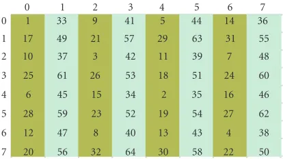
0 1 2 3 4 5 6 7
0 1 33 9 41 5 44 14 36
1 17 49 21 57 29 63 31 55
2 10 37 3 42 11 39 7 48
3 25 61 26 53 18 51 24 60
4 6 45 15 34 2 35 16 46
5 28 59 23 52 19 54 27 62
6 12 47 8 40 13 43 4 38
7 20 56 32 64 30 58 22 50
Figure5: Computation order of coefficients.
overhead is required for actually computing the scaled DCT. It is possible, though, to apply different precomputed DCTs to different blocks employing block classification that indi-cates which precomputed DCT should perform best with a classified block (seeSection 5.3).
4.1.3. Experiments
For experiments, the fast 2D algorithm given by Cho and Lee [9], in combination with the Arai-Agui-Nakajima (AAN) 1D algorithm [10], has been used, and this algorithm com-bination is extended in the following with computational complexity scalability. Both algorithms were adopted be-cause their combination provides a highly efficient DCT computation (104 multiplications and 466 additions). The results of this experiment presented below are discussed with the assumption that an addition is equal to one op-eration and a multiplication is equal to three opop-erations (in powerful cores, additions and multiplications have equal weight).
The scalability-optimized computation order in this ex-periment is shown in Figure 5, where the matrix has been shaded with different gray levels to mark the first and the second half of the coefficients in the sorted list. It can be seen that in this case, the computation order clearly favors hori-zontal or vertical edges (depending on whether the matrix is transposed or not).
Figure 6shows the scalability of our DCT computation technique using the scalability-optimized computation or-der, and the zigzag order as reference computation order. InFigure 6a, it can be seen that the number of coefficients that are computed with the scalability-optimized computa-tion order is higher at any computacomputa-tion limit than the zigzag order.Figure 6bshows the resulting peak signal-to-noise ra-tio (PSNR) of the first frame from the “Voit” sequence us-ing both computation orders, where no quantization step is performed. A 1–5 dB improvement in PSNR can be noticed, depending on the amount of available operations.
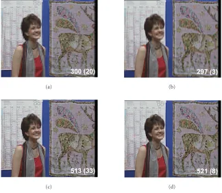
Finally,Figure 7shows two picture pairs (based on zigzag and scalability-optimized orders preferring horizontal de-tails) sampled from the “Renata” sequence during diff er-ent stages of the computation (represer-enting low-cost and medium-cost applications). Perceptive evaluations of our
ex-periments have revealed that the quality improvement of our technique is the largest between 200 and 600 operations per block. In this area, the amount of coefficients is still rela-tively small so that the benefit of having much more coef-ficients computed than in a zigzag order is fully exploited. Although the zigzag order yields perceptually important co-efficients from the beginning, the computed number is sim-ply too low to show relevant details (e.g., see the background calendar in the figure).
4.2. Scalable classification of picture blocks
4.2.1. Basics
The conventional MPEG encoding system processes each im-age block in the same content-independent way. However, content-dependent processing can be used to optimize the coding process and output quality, as indicated below.
(i) Block classification is used for quantization to distin-guish between flat, textured, and mixed blocks [11] and then apply different quantization factors for these blocks for optimizing the picture quality at given bit rate limitations. For example, quantization errors in textured blocks have a small impact on the perceived image quality. Blocks containing both flat and textured parts (mixed blocks) are usually blocks that contain an edge, where the disturbing ringing effect gets worse with high quantization factors.
(ii) The ME (see Section 4.3) can take the advantage of classifying blocks to indicate whether a block has a structured content or not. The drawback of conven-tional ME algorithms that do not take the advantage of block classification is that they spend many compu-tations on computing MVs for, for example, relatively flat blocks. Unfortunately, despite the effort, such ME processes yield MVs of poor quality. Employing block classification, computations can be concentrated on blocks that may lead to accurate MVs [12].
Of course, in order to be useful, the costs to perform block classification should be less than the saved computations. Given the above considerations, in the following, we will adopt content-dependent adaptivity for coding and motion processing. The next section explains the content adaptivity in more detail.
4.2.2. Scalability
We perform a simple block classification based on detecting horizontal and vertical transitions (edges) for two reasons.
(i) From the scalable DCT, computation orders are avail-able that prefer coefficients representing horizontal or vertical edges. In combination with a classification, the computation order that fits best for the block content can be chosen.
70 60 50 40 30 20 10 0
N
umber
of
calculat
ed
coe
ffi
cients
0 100 200 300 400 500 600 700 800 Operation count per processed (8×8)-DCT block Scalability-optimized
Zigzag
(a)
Picture “voit” 50 45 40 35 30 25 20 15 10
SNR
(dB)
o
f
a
co
mplet
e
fr
ame
0 100 200 300 400 500 600 700 800 Operation count per processed (8×8)-DCT block Scalability-optimized
Zigzag
(b)
Figure6: Comparison of the scalability-optimized computation order with the zigzag order. At limited computation resources, more DCT
coefficients are computed (a) and a higher PSNR is gained (b) with the scalability-optimized order than with the zigzag order.
(a) (b)
(c) (d)
Figure7: A video frame from the “Renata” sequence coded employing the scalability-optimized order (a) and (c), and the zigzag order
(b) and (d). Indexm(n) meansmoperations are performed forncoefficients. The scalability-optimized computation order results in an
improved quality (compare sharpness and readability).
good MVs for every position along such an edge (where a displacement in this direction does not in-troduce large displacement errors), searching for MVs acrossthis edge will rapidly reduce the displacement error and thus lead to an appropriate MV. Horizon-tal and vertical edges can be detected by significant changes of pixel values in vertical and horizontal di-rections, respectively.
The edge detecting algorithm we use is in principle based on continuously summing up pixel differences along rows or columns and counting how often the sum exceeds a certain threshold. Letpi, withi=0, 1,. . ., 15, be the pixel values in a
row or column of a macroblock (size 16×16). We then define a range where pixel divergence (di) is considered as noise if |di|is below a thresholdt. The pixel divergence is defined by
(a) (b)
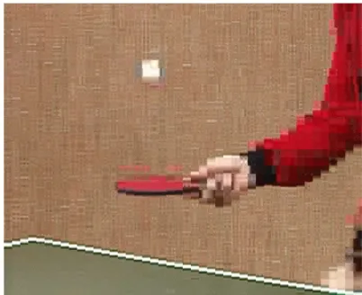
Figure8: Visualization of block classification using a picture of the “table tennis” sequence. The left (right) picture shows blocks where horizontal (vertical) edges are detected. Blocks that are visible in both pictures belong to the class “diagonal/structured,” while blocks that are blanked out in both pictures are considered as “flat.”
Table1: Definition of pixel divergence, where the divergence is con-sidered as noise if it is below a certain threshold.
Condition Pixel divergencedi
i=0 0
(i=1,. . ., 15)∧(|di−1| ≤t) di−1+ (pi−pi−1) (i=1,. . ., 15)∧(|di−1|> t) di−1+ (pi−pi−1)−sgn(di−1)∗t
The area preceding the edge yields a level in the inter-val [−t; +t]. The middle of this interval is atd=0, which is modified by adding±tin the case that|d|exceeds the inter-val around zero (start of the edge). This mechanism will fol-low the edges and prevent noise from being counted as edges. The countercas defined below indicates how often the actual interval was exceeded:
c= 15
i=1
0 ifdi≤t,
1 ifdi> t.
(5)
The occurrence of an edge is defined by the resulting value of cfrom (5).
This edge detecting algorithm is scalable by selecting the threshold t, the number of rows and columns that are considered for the classification, and a typical value for c. Experimental evidence has shown that in spite of the com-plexity scalability of this classification algorithm, the evalu-ation of a single row or column in the middle of a picture block was found sufficient for a rather good classification.
4.2.3. Experiments
Figure 8 shows the result of an example to classify image blocks of size 16×16 pixels (macroblock size). For this
ex-periment, a threshold oft =25 was used. We considered a block to be classified as a “horizontal edge” ifc ≥ 2 holds for the central column computation and as a “vertical edge” if c≥ 2 holds for the row computation. Obviously, we can derive two extra classes: “flat” (for all blocks that do not be-long to the CLASS “horizontal edge” NOR the class “verti-cal edge”) and diagonal/structured (for blocks that belong to both classes horizontal edge and vertical edge).
The visual results ofFigure 8 are just an example of a more elaborate set of sequences with which experiments were conducted. The results showed clearly that the algorithm is sufficiently capable of classifying the blocks for further content-adaptive processing.
4.3. Motion estimation
4.3.1. Basics
The ME process in MPEG systems divides each frame into rectangular macroblocks (16×16 pixels each) and computes MVs per block. An MV signifies the displacement of the block (in the x-y pixel plane) with respect to a reference image. For each block, a number of candidate MVs are ex-amined. For each candidate, the block evaluated in the cur-rent image is compared with the corresponding block fetched from the reference image displaced by the MV. After testing all candidates, the one with the best match is selected. This match is done on basis of the SAD between the current block and the displaced block. The collection of MVs for a frame forms an MV field.
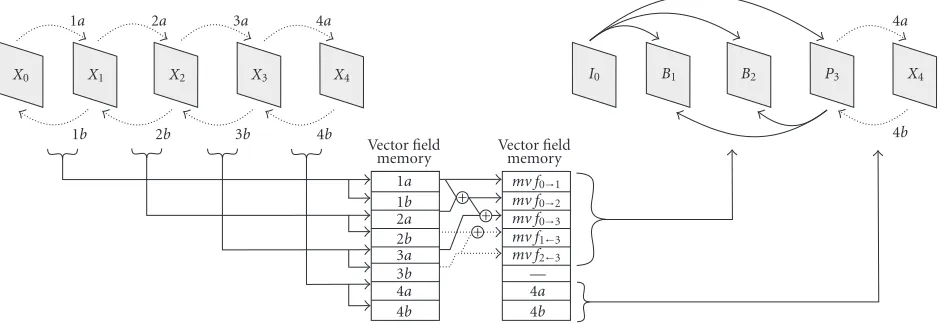
X0 X1 X2 X3 X4
1a 2a 3a 4a
1b 2b 3b 4b Vector field
memory 1a
1b
2a
2b
3a
3b
4a
4b
+ + +
Vector field memory
mv f0→1
mv f0→2
mv f0→3
mv f1←3
mv f2←3 — 4a
4b
I0 B1 B2 P3 X4
4a
4b
Figure9: An overview of the new scalable ME process. Vector fields are computed for successive frames (left) and stored in memory. After defining the GOP structure, an approximation is computed (middle) for the vector fields needed for MPEG coding (right). Note that for this example it is assumed that the approximations are performed after the exemplary GOP structure is defined (which enables dynamic GOP
structures), therefore the vector field (1b) is computed but not used afterwards. With predefined GOP structures, the computation of (1b) is
not necessary.
4.3.2. Scalability
The scalable ME is designed such that it takes the advan-tage of the intrinsically high prediction quality of ME be-tween successive frames (smallest temporal distance), and thereby works not only for the typical (predetermined and fixed) MPEG GOP structures, but also for more general cases. This feature enables on-the-fly selection of GOP struc-tures depending on the video content (e.g., detected scene changes, significant changes of motion, etc.). Furthermore, we introduce a new technique for generating MV fields from other vector fields by multitemporalapproximation (not to be confused with other forms of multitemporal ME as found in H.264). These new techniques give more flexibility for a scalable MPEG encoding process.
The estimation process is split up into three stages as fol-lows.
Stage 1 Prior to defining a GOP structure, we perform a sim-ple recursive motion estimation (RME) [16] for every received frame to compute the forward and backward MV field between the received frame and its predeces-sor (see the left-hand side ofFigure 9). The computa-tion of MV fields can be omitted for reducing compu-tational effort and memory.
Stage 2 After defining a GOP structure, all the vector fields required for MPEG encoding are generated through multitemporal approximations by summing up vec-tor fields from the previous stage. Examples are given in the middle of Figure 9, for example, vector field (mv f0→3)=(1a) + (2a) + (3a). Assume that the vector field (2a) has not been computed in Stage 1 (due to a chosen scalability setting), one possibility to approxi-mate (mv f0→3) is (mv f0→3)=2∗(1a) + (3a). Stage 3 For final MPEG ME in the encoder, the computed
approximated vector fields from the previous stage are
used as an input. Beforehand, an optional refinement of the approximations can be performed with a second iteration of simple RME.
We have employed simple RME as a basis for intro-ducing scalability because it offers a good quality for time-consecutive frames at low computing complexity.
The presented three-stage ME algorithm differs from known multistep ME algorithms like in [17], where initially estimated MPEG vector fields are processed for a second time. Firstly, we do not have to deal with an increasing tem-poral distance when deriving MV fields in Stage 1. Secondly, we process the vector fields in a display order having the ad-vantage of frame-by-frame ME, and thirdly, our algorithm provides scalability. The possibility of scaling vector fields, which is part of our multitemporal predictions, is mentioned in [17] but not further exploited. Our algorithm makes ex-plicit use of this feature, which is a fourth difference. In the sequel, we explain important system aspects of our al-gorithm.
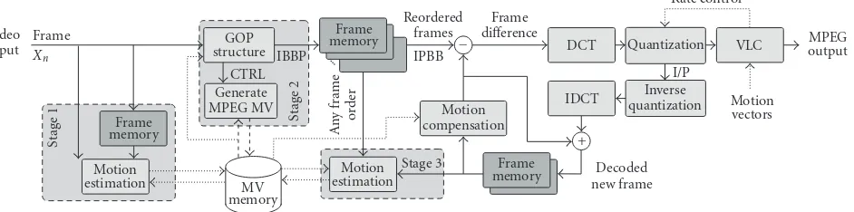
Figure 10shows the architecture of the three-stage ME al-gorithm embedded in an MPEG encoder. With this architec-ture, the initial ME process in Stage 1 results in a high-quality prediction because original frames without quantization er-rors are used. The computed MV fields can be used in Stage 2 to optimize the GOP structures. The optional refinement of the vector fields in Stage 3 is intended for high-quality ap-plications to reach the quality of a conventional MPEG ME algorithm.
…
Figure10: Architecture of an MPEG encoder with the new scalable three-stage motion estimation.
31
A B Exemplary regions with slow (A) or fast (B) motion.
Figure 11: PSNR of motion-compensated B-frames of the
“Ste-fan” sequence (tennis scene) at different computational efforts—
P-frames are not shown for the sake of clarity (N =16,M =4).
The percentage shows the different computational effort that
re-sults from omitting the computation of vector fields in Stage 1 or performing an additional refinement in Stage 3.
complexity, which makes it affordable for mobile devices that up till now rarely make use of B-frames. A further optimiza-tion is seen (but not worked out) in limiting the ME process of Stages 1 and 3 to significant parts of a vector field in order to further reduce the computational effort and memory.
4.3.3. Experiments
To demonstrate the flexibility and scalability of the three-stage ME technique, we conducted an initial experiment us-ing the “Stefan” sequence (tennis scene). A GOP size ofN=
16 and M = 4 (thus “IBBBP” structure) was used, com-bined with a simple pixel-based search. In this experiment, the scaling of the computational complexity is introduced by gradually increasing the vector field computations in Stage 1 and Stage 3. The results of this experiment are shown in Figure 11. The area in the figure with the white background shows the scalability of the quality range that results from downscaling the amount of computed MV fields. Each vector
27
100% 114% 129% 143% 157% 171% 186% 200%
Complexity of motion estimation process SNR B- and P-frames
Figure12: Average PSNR of motion-compensated P- and B-frames
and the resulting bit rate of the encoded “Stefan” stream at diff
er-ent computational efforts. A lower average PSNR results in a higher
differential signal that must be coded, which leads to a higher bit
rate. The percentage shows the different computational effort that
results from omitting the computation of vector fields in Stage 1 or performing an additional refinement in Stage 3.
field requires 14% of the effort compared to a 100% simple RME [16] based on four forward vector fields and three back-ward vector fields when going from one to the next reference frame. If all vector fields are computed and the refinement Stage 3 is performed, the computational effort is 200% (not optimized).
Table2: Average luminance PSNR of the motion-compensated P- and B-frames for sequences “Stefan” (A), “Renata” (B), and “Teeny” (C)
with different ME algorithms. The second column shows the average number of SAD-based vector evaluations per MV (based on (A)).
Algorithm Tests/MV (A) (B) (C)
2D FS (32×32) 926.2 24.80 29.62 26.78
NTSS [14] 25.2 22.55 27.41 24.22
Diamond [15] 21.9 22.46 27.34 26.10
Simple RME [16] 16.0 21.46 27.08 23.89
Three-stage ME 200% (employing [16]) 37.1 25.16 29.24 26.92
Three-stage ME 100% (employing [16]) 20.1 23.52 27.45 24.74
sequence is 0.012 bits per pixel (bpp) lower when using the new technique (0.096 bpp instead of 0.108 bpp). When re-ducing the computational effort to 57% of a single-pass sim-ple RME, an increase of the bit rate by 0.013 bpp compared to the 32×32 full search (FS) is observed.
Further comparisons are made with the scalable three-stage ME running at full and “normal” quality.Table 2shows the average PSNR of the motion-compensated P- and B-frames for three different video sequences and ME algo-rithms with the same conditions as described above (same N,M, etc.). The first data column (tests per MV) shows the average number of vector tests that are performed per mac-roblock in the “Stefan” sequence to indicate the performance of the algorithms. Note that MV tests pointing outside the picture are not counted, which results in numbers that are lower than the nominal values (e.g., 926.2 instead of 1024 for 32×32 FS). The simple RME algorithm results in the low-est quality here because only three vector field computations out of 4∗(4 + 3)=28 can use temporal vector candidates as prediction. However, our new three-stage ME that uses this simple RME performs, comparable to FS, at 200% complex-ity, and at 100%, it is comparable to the other fast ME algo-rithms.
The results inTable 2are based on the simple RME al-gorithm from [16]. A modified algorithm has been found later [18] that forms an improved replacement for the sim-ple RME. This modified algorithm is based on the block classification as presented inSection 4.2. This algorithm was used for further experiments and is summarized as follows. Prior to estimating the motion between two frames, the mac-roblocks inside a frame are classified into areas having hor-izontal, vertical edges, or no edges. The classification is ex-ploited to minimize the number of MV evaluations for each macroblock by, for example, concentrating vector evalua-tions across the detected edge. A novelty in the algorithm is adistributionof good MVsto other macroblocks, even al-ready processed ones, which differs from other known recur-sive ME techniques that reuse MVsfrom previouslyprocessed blocks.
5. SYSTEM ENHANCEMENTS AND EXPERIMENTS
The key approach to optimize a system is to reuse and com-bine data that is generated by the system modules in order to control other modules. In the following, we present several
approaches, where data can be reused or generated at a low cost in a coding system for an optimization purpose.
5.1. Experimental environment
The scalable modules for the (I)DCT, (de)quantization, ME, and VLC are integrated into an MPEG encoder framework, where the scaling of the IDCT and the (de)quantization is effected from the scalable DCT (see Section 5.2). In order to visualize the obtained scalability of the computations, the scalable modules are executed at different parameter settings, leading to effectively varying the number of DCT coefficients and MV candidates evaluated. When evaluating the system complexity, the two different numbers have to be combined into a joint measure. In the following, the elapsed execu-tion time of the encoder needed to code a video sequence is used as a basis for comparison. Although this time param-eter highly depends on the underlying architecture and on the programming and operating system, it reflects the com-plexity of the system due to the high amount of operations involved.
The experiments were conducted on a Pentium-III Linux system running at 733 MHz. In order to be able to measure the execution time of single functions being part of the com-plete encoder execution, it was necessary to compile the C++ program of the encoder without compiler optimizations. Ad-ditionally, it should be noted that the experimental C++ code was not optimized for fast execution or usage of architecture-specific instructions (e.g., MMX). For these reasons, the en-coder and its measured execution times cannot be compared with existing software-based MPEG encoders. However, we have ensured that the measured change in the execution time results from the scalability of the modules, as we did not change the programming style, code structures, or common coding parameters.
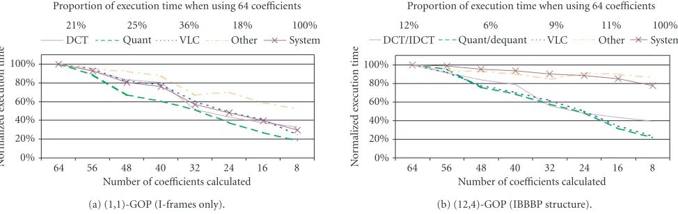
5.2. Effect of scalable DCT
Proportion of execution time when using 64 coefficients
21% 25% 36% 18% 100%
DCT Quant VLC Other System
100%
Number of coefficients calculated (a) (1,1)-GOP (I-frames only).
Proportion of execution time when using 64 coefficients
12% 6% 9% 11% 100%
DCT/IDCT Quant/dequant VLC Other System 100%
Number of coefficients calculated (b) (12,4)-GOP (IBBBP structure).
Figure13: Complexity reduction of the encoder modules relative to the full DCT processing, with (1,1)-GOPs (a) and with (12,4)-GOPs) (b). Note that in this case, 62% of the coding time is spent in (b) for ME and MC (not shown for convenience). For visualization of the complexity reduction, we normalize the execution time for each module to 100% for full processing.
detect zero coefficients. This saves computations as follows.
(i) The quantization and dequantization require a fixed amount of operations per processed intra- or interco-efficient. Thus, each skipped coefficientc∈C\Ssaves 1/64 of the total complexity of the quantization and dequantization modules.
(ii) The VLC processes the DCT coefficients in a zigzag or an alternate order and generates run-value pairs for coefficients that are unequal to zero. “Run” indicates the number of zero coefficients that are skipped before reaching a nonzero coefficient. The usage of a scaled DCT increases the probability that zero coefficients oc-cur, for which no computations are spent.
(iii) The IDCT can be simplified by knowing which coef-ficients are zero. It is obvious that, for example, each multiplication with a known factor of 0 and additions with a known addend of 0 can be skipped.
The execution time of the modules when coding the “Stefan” sequence and scaling the modules that process coefficients is visualized in Figure 13. The category “other” is used for functions that are not exclusively used by the scaled modules. Figure 13ashows the results of an experiment, where the se-quence was coded with I-frames only. Similar results are ob-served inFigure 13bfrom another experiment, for which P-and B-frames are included. To remove the effect of quanti-zation, the experiments were performed with qscale=1. In this way, the figures show results that are less dependent on the coded video content.
The measured PSNR of the scalable encoder running at full quality is 46.5 dB for Figure 13a and 48.16 dB for Figure 13b. When the number of computed coefficients is gradually reduced from 64 to 8, the PSNR drops gradually to 21.4 dB Figure 13a, respectively, 21.81 dB in Figure 13b. In Figures 13aand13b, the quality gradually reduces from “no noticeable differences” down to “severe blockiness.” In Figure 13b, the curve for the ME module is not shown for
convenient because the ME (in this experiment, we used dia-mond search ME [15]) is not affected from processing a dif-ferent number of DCT coefficients.
5.3. Selective DCT computation based on block classification
The block classification introduced inSection 4.2is used to enhance the output quality of the scaled DCT by using diff er-ent computation orders for blocks in different classes. A sim-ple experiment indicates the benefit in quality improvement. In the experiment, we computed the average values of DCT coefficients when coding the “table tennis” sequence with I-frames only. Each DCT block is taken after quantization with qscale = 1.Figure 14shows the statistic for blocks that are classified as having a horizontal (left graph) or vertical (right graph) edge only. It can be seen that the classification leads to a frequency concentration in the DCT coefficient matrix in the first column, respectively, row.
We found that the DCT algorithm of Arai et al. [10] can be used best for blocks with horizontal or vertical edges, while background blocks have a better quality impression when using the algorithm by Cho and Lee [9]. The exper-iment made for Figure 15shows the effect of the two algo-rithms on the table edges ([10] is better) and the background ([9] is better). In both cases, the computation orders de-signed for preferring horizontal edges are used. The compu-tation limit was set to 256 operations, leading to 9 computed coefficients for [10] and 11 for [9], respectively. The coeffi -cients that are computed are marked in the corresponding DCT matrix. It can be seen that [10] covers all main vertical frequencies, while [9] covers a mixture of high and low ver-tical and horizontal frequencies. The resulting overall PSNR are 26.58 dB and 24.32 dB, respectively.
v0 v1
v2 v3
v4 v5
v6 v7 h7 h6h5 h4h3
h2h1 h0
140 120 100 80 60 40 20 0
7
v 0
h
7 v0
v1v2 v3
v4 v5
v6 v7 h7 h6 h5 h4h3
h2h1 h0
140 120 100 80 60 40 20 0
Class “horizontal” Class “vertical”
Figure14: Statistics of the average absolute values of the DCT coefficients taken after quantization with qscale=1. Here, the “table tennis” sequence was coded with I-frames only. The left (right) graph shows the statistic for blocks classified as having horizontal (vertical) edges.
Arai-Agui-Nakajima (AAN) (a)
ChoLee (b)
Figure15: Example of scaled AAN-DCT (a) and ChoLee-DCT (b) at 256 operations. AAN fits better for horizontal edges, while ChoLee has better results for the background.
to compute 11 coefficients. Blocks with both detected zontal and vertical edges are treated as blocks having hori-zontal edges only because an optimized computation order for such blocks is not yet defined. The resulting PSNR is 26.91 dB.
5.4. Dynamic interframe DCT coding
Besides intraframe coding, the DCT computation on frame differences (for interframe coding) occurs more often than intraframe coding (N−1 times for (N,M) GOPs). For this reason, we look more closely to interframe DCT coding, where we discovered a special phenomenon from the scal-able DCT. It was found that the DCT coded frame differences show temporal fluctuations in frequency content. The tem-poral fluctuation is caused by the motion in the video con-tent combined with the special selection function of the co-efficients computed in our scalable DCT. Due to the motion, the energy in the coefficients shifts over the selection pattern
so that the quality gradually increases over time. Figure 17 shows this effect from an experiment when coding the “Ste-fan” sequence with IPP frames (GOP structure (GOP sizeN, IP distance M)= (12, 1)) while limiting the computation to 32 coefficients. The camera movement in the shown se-quence is panning to the right. It can be seen for example that the artifacts around text decrease over time.
Figure16: Both DCT algorithms were used to code this frame. Af-ter block classification, the ChoLee-DCT was used to code blocks where no edges were detected and the AAN-DCT for blocks with detected edges.
Figure17: Visualization of a phenomenon from the scalable DCT, leading to a gradual quality increase over time.
having zero motion like nonmoving background) and there-fore having no temporal fluctuations in their frequency con-tent will obtain the same result as a nonpartitioned DCT computation after full computation of the partitioned DCT.
Based on the idea of temporal data partitioning, we de-fineNsubsetssi(withi=0,. . .,N−1) of coefficients such
that
N−1
i=0
si=S, (6)
where the setScontains all the 64 DCT coefficients. The sub-setssiare used to build up functions fithat compute a scaled
DCT for the coefficients insi. The functionsfiare applied to
blocks with static contents in cyclical sequence (one per in-tercoded frame). AfterNintercoded frames, each coefficient for these blocks is computed at least once.
We set up an experiment using the “table tennis” se-quence as follows in order to measure the effect of dynamic interframe coding. The computation of the DCT (for
in-Figure18: Example of coefficient subsets (marked gray) used for
dynamic interframe DCT coding with a limitation to 32 coefficients
per subset.
40 38 36 34 32 30 28 26 24 22 20
PSNR
(dB)
1 21 41 61 81 101 121 141 161 181 201 221 241 261 281 Frame number
Dynamic Horizontal I-frames
Figure19: PSNR measures for the coded “table tennis” sequence,
where the DCT computation was scaled to compute 32 coefficients.
Compared to coding I-frames only (medium gray curve), inter DCT coding results in an improved output quality in case of motion (light gray curve) and even a higher output quality with dynamic interframe DCT computation.
70 Average number of MV evaluations per macroblock ME
Figure 20: Example of ME scalability for the complete encoder when using a (12, 4)-GOP (“IBBBP” structure) for coding.
coefficients for the I-frames. Although this seems interesting, this was not further pursued because of limited time.
5.5. Effect of scalable ME
The execution time of the MPEG modules when coding the “Stefan” sequence and scaling the ME is visualized in Figure 20. It can be seen that the curve for the ME block scales linearly with the number of MV evaluations, whereas the other processing blocks remain constant. The average number of vector candidates that are evaluated per mac-roblock by the scalable ME in this experiment is between 0.42 and 12.53. This number is clearly below the achieved average number of candidates (21.77) when using the di-amond search [15]. At the same time, we found that our scalable codec results in a higher quality of the MC frame (up to 25.22 dB PSNR in average) than the diamond search (22.53 dB PSNR in average), which enables higher compres-sion ratios (see the next section).
5.6. Combined effect of scalable DCT and scalable ME
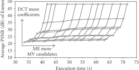
In this section, we combine the scalable ME and DCT in the MPEG encoder and apply the scalability rules for (de)quantization, IDCT, and VLC, as we have described them inSection 2. Since the DCT and ME are the main sources for scalability, we will focus on the tradeoffbetween MVs and the number of computed coefficients.
Figure 21 portrays the obtained average PSNR of the coded “Stefan” sequence (CIF resolution) and Figure 22 shows the achieved bit rate corresponding toFigure 21. The experiments are performed with a (12,4)-GOP and qscale=
1. Both figures indicate the large design space that is available with the scalable encoder without quantization and open-loop control. The horizontally oriented curves refer to a fixed number of DCT coefficients (e.g., 8, 16, 24, 32,. . ., 64), whereas vertically oriented curves refer to a fixed number of MV candidates. A normal codec would compute all the 64 coefficients and would therefore operate on the top horizon-tal curve of the graph. The figures should be jointly evalu-ated. Under the above-mentioned measurement conditions, the potential benefit of the scalable ME is only visible in the
50
Figure21: PSNR results of different configurations for the scalable MPEG modules.
Figure 22: Obtained bit rates of different configurations for the scalable modules. The markers refer to points in the design space, where the same bit rate and quality (not computational complex-ity) is obtained as resulting from using diamond search (A) or full
search with a 32×32 (B) or 64×64 (C) search area for ME.
reduction of the bit rate (seeFigure 22) since an improved ME leads to less DCT coefficients for coding the difference signal after the MC in the MPEG loop.
Figures21and22both present a large design space, but in practice, this is limited due to the quantization and bit rate control. Further experiments using quantization and bit rate control at 1500 kbps for the “Stefan,” “Foreman,” and “ta-ble tennis” sequence resulted in a quality level range from roughly 22 dB to 38 dB. As could be expected from inserting the quantization, the curves moved to lower PSNR (the lower half ofFigure 21) and less computation time is required since fewer coefficients are computed. It was found that the re-maining design space is larger for sequences having less mo-tion.
6. CONCLUSIONS
We have presented techniques for complexity scalable MPEG encoding that gradually reduce the quality as a function of limited resources. The techniques involve modifications to the encoder modules in order to pursue scalable complexity and/or quality. Special attention has been paid to exploiting a scalable DCT and ME because they represent two compu-tational expensive corner stones of MPEG encoding. The in-troduced new techniques for the scalability of the two func-tions show considerable savings of computational complex-ity for video applications having low-qualcomplex-ity requirements. In addition, a scalable block classification technique has been presented, which is designed to support the scalable process-ing of the DCT and ME. In the second step, performance evaluations have been carried out by constructing a com-plete MPEG encoding system in order to show the design space that is achieved with the scalability techniques. It has been shown that even a higher reduction in computational complexity of the system could be obtained if available data (e.g., which DCT coefficients are computed during a scal-able DCT computation) is exploited to optimize other core functions.
The obtained execution times of the encoder when cod-ing the “Stefan” sequence as an example for complexity has been measured. It was found that the overall execution time of the scalable encoder can be gradually reduced to roughly 50% of its original execution time. At the same time, the codec provides a wide range of video quality levels (roughly from 20 dB to 48 dB PSNR in average) and compression ra-tios (from 0.58 to 2.02 Mbps). Further experiments target-ing a bit rate of 1500 kbps for the Stefan, Foreman, and table tennis sequence result in a quality level range from roughly 21.5 dB to 38.5 dB. Compared with the diamond search ME from literature which requires 21.77 MV candidates on the average per macroblock, our scalable coder operating un-der the same quality and bit rate combination uses 10.06 average MV candidates, thus 53.8% less than the diamond search.
Another result of our experiments is that the scalable DCT has an integrated coefficient selection function which may enable a quality increase during interframe coding. This phenomenon can lead to an MPEG encoder with a number of special DCTs with different selection functions, and this option should be considered for future work. This should
also include different scaling of the DCT for intra- and inter-frame coding. For scalable ME, future work should examine the scalability potentials of using various fixed and dynamic GOP structures, and of concentrating or limiting the ME to frame parts, whose content (could) have the current viewer focus.
REFERENCES
[1] C. Hentschel, R. Braspenning, and M. Gabrani, “Scalable
al-gorithms for media processing,” inIEEE International
Confer-ence on Image Processing (ICIP ’01), vol. 3, pp. 342–345, Thes-saloniki, Greece, October 2001.
[2] R. Prasad and K. Ramkishor, “Efficient implementation of
MPEG-4 video encoder on RISC core,” inIEEE International
Conference on Consumer Electronics, Digest of Technical papers (ICCE ’02), pp. 278–279, Los Angeles, Calif, USA, June 2002. [3] K. Lengwehasatit and A. Ortega, “DCT computation based
on variable complexity fast approximations,” inProc. IEEE
International Conference of Image Processing (ICIP ’98), vol. 3, pp. 95–99, Chicago, Ill, USA, October 1998.
[4] S. Peng, “Complexity scalable video decoding via IDCT data
pruning,” inInternational Conference on Consumer Electronics
(ICCE ’01), pp. 74–75, Los Angeles, Calif, USA, June 2001. [5] Y. Chen, Z. Zhong, T. H. Lan, S. Peng, and K. van Zon,
“Reg-ulated complexity scalable MPEG-2 video decoding for media
processors,” IEEE Trans. Circuits and Systems for Video
Tech-nology, vol. 12, no. 8, pp. 678–687, 2002.
[6] R. Braspenning, G. de Haan, and C. Hentschel, “Complexity
scalable motion estimation,” inProc. of SPIE: Visual
Commu-nications and Image Processing 2002, vol. 4671, pp. 442–453, San Jose, Calif, USA, 2002.
[7] S. Mietens, P. H. N. de With, and C. Hentschel, “New DCT
computation technique based on scalable resources,” Journal
of VLSI Signal Processing Systems for Signal, Image, and Video Technology, vol. 34, no. 3, pp. 189–201, 2003.
[8] S. Mietens, P. H. N. de With, and C. Hentschel, “Frame
reordered multi-temporal motion estimation for scalable
MPEG,” inProc. 23rd International Symposium on
Informa-tion Theory in the Benelux, Louvain-la-Neuve, Belgium, May 2002.
[9] N. Cho and S. Lee, “Fast algorithm and implementation of
2-D discrete cosine transform,” IEEE Trans. Circuits and
Sys-tems, vol. 38, no. 3, pp. 297–305, 1991.
[10] Y. Arai, T. Agui, and M. Nakajima, “A fast DCT-SQ scheme for
images,”Transactions of the Institute of Electronics, Information
and Communication Engineers, vol. 71, no. 11, pp. 1095–1097, 1988.
[11] D. Farin, N. Mache, and P. H. N. de With, “A software-based high-quality MPEG-2 encoder employing scene change
detec-tion and adaptive quantizadetec-tion,” IEEE Transactions on
Con-sumer Electronics, vol. 48, no. 4, pp. 887–897, 2002.
[12] T. Kummerow and P. Mohr, Method of determining motion
vectors for the transmission of digital picture information, EPO 496 051, European Patent Application, November 1991. [13] M. Chen, L. Chen, and T. Chiueh, “One-dimensional full
search motion estimation algorithm for video coding,” IEEE
Trans. Circuits and Systems for Video Technology, vol. 4, no. 5, pp. 504–509, 1994.
[14] R. Li, B. Zeng, and M. Liou, “A new three-step search
algo-rithm for block motion estimation,”IEEE Trans. Circuits and
Systems for Video Technology, vol. 4, no. 4, pp. 438–442, 1994. [15] J. Tham, S. Ranganath, M. Ranganath, and A. A. Kassim, “A novel unrestricted center-biased diamond search algorithm
for block motion estimation,” IEEE Trans. Circuits and
[16] P. N. H. de With, “A simple recursive motion estimation
tech-nique for compression of HDTV signals,” inIEE 4th
Interna-tional Conference on Image Processing and Its Applications (IPA
’92), pp. 417–420, Maastricht, The Netherlands, April 1992.
[17] F. Rovati, D. Pau, E. Piccinelli, L. Pezzoni, and J. M. Bard, “An innovative, high quality and search window independent mo-tion estimamo-tion algorithm and architecture for MPEG-2
en-coding,” IEEE Transactions on Consumer Electronics, vol. 46,
no. 3, pp. 697–705, 2000.
[18] S. Mietens, P. H. N. de With, and C. Hentschel,
“Com-putational complexity scalable motion estimation for mobile
MPEG encoding,”IEEE Transactions on Consumer Electronics,
2002/2003.
Stephan Mietens was born in Frankfurt (Main), Germany in 1972. He graduated in Computer Science from the Technical Uni-versity of Darmstadt, Germany, in 1998 on the topic of “asynchronous VLSI design.” Subsequently, he joined the University of Mannheim, where he started his research on “flexible video coding and architectures” in cooperation with Philips Research Labora-tories in Eindhoven, The Netherlands. He
joined the Eindhoven University of Technology in Eindhoven, The Netherlands, in 2000, where he is working towards a Ph.D. degree on “scalable video systems.” Since 2003, he became a Scientific Re-searcher at Philips Research Labs. in the Storage and System Ap-plications group, where he is involved in projects to develop new coding techniques.
Peter H. N. de Withobtained his M.S. engi-neering degree from the University of Tech-nology in Eindhoven in 1984 and his Ph.D. degree from the University of Technology Delft, The Netherlands in 1992. From 1984 to 1993, he joined the Magnetic Recording Systems Department, Philips Research Labs. in Eindhoven, and was involved in several European projects on SDTV and HDTV recording. He also contributed as a
prin-cipal coding expert to the DV digital camcording standard. In 1994, he joined the TV Systems group, where he was leading ad-vanced programmable architectures design as Senior TV Systems Architect. In 1997, he became a Full Professor at the University of Mannheim, Germany, in the Faculty of Computer Engineering. In 2000, he joined CMG Eindhoven as a principal consultant and he became a Professor in Electrical Engineering Faculty, University of Technology Eindhoven (EE Faculty). He has written numerous pa-pers on video coding, architectures, and their realization. He is a Regular Teacher of postacademic courses at external locations. In 1995 and 2000, he coauthored papers that received the IEEE CES Transactions Paper Award. In 1996, he obtained a company Inven-tion Award. Mr. de With is an IEEE Senior Member, Program Mem-ber of the IEEE CES (Tutorial Chair, Program Chair) and Chairman of the Benelux Information Theory Community.
Christian Hentschelreceived his Dr.-Ing. (Ph.D.) in 1989 and Dr.-Ing. habil. in 1996 from Braunschweig University of Technol-ogy, Germany. He worked on digital video signal processing with focus on quality improvement. In 1995, he joined Philips
Research Labs. in Briarcliff Manor, USA,
where he headed a research project on moir´e analysis and suppression for CRT-based displays. In 1997, he moved to Philips
Research Labs. in Eindhoven, The Netherlands, leading a cluster for programmable video architectures. He got the position of a Princi-pal Scientist and coordinated a project on scalable media processing
with dynamic resource control between different research