LETTER
Fatality rates of the
M
w
~8.2, 1934,
Bihar–Nepal earthquake and comparison
with the April 2015 Gorkha earthquake
Soma Nath Sapkota
1*, Laurent Bollinger
2and Frédéric Perrier
3Abstract
Large Himalayan earthquakes expose rapidly growing populations of millions of people to high levels of seismic hazards, in particular in northeast India and Nepal. Calibrating vulnerability models specific to this region of the world is therefore crucial to the development of reliable mitigation measures. Here, we reevaluate the >15,700 casualties (8500 in Nepal and 7200 in India) from the Mw ~8.2, 1934, Bihar–Nepal earthquake and calculate the fatality rates for this earthquake using an estimation of the population derived from two census held in 1921 and 1942. Values reach 0.7–1 % in the epicentral region, located in eastern Nepal, and 2–5 % in the urban areas of the Kathmandu valley. Assuming a constant vulnerability, we obtain, if the same earthquake would have repeated in 2011, fatalities of 33,000 in Nepal and 50,000 in India. Fast-growing population in India indeed must unavoidably lead to increased levels of casualty compared with Nepal, where the population growth is smaller. Aside from that probably robust fact, extrapolations have to be taken with great caution. Among other effects, building and life vulnerability could depend on population concentration and evolution of construction methods. Indeed, fatalities of the April 25, 2015, Mw 7.8 Gorkha earthquake indicated on average a reduction in building vulnerability in urban areas, while rural areas remained highly vulnerable. While effective scaling laws, function of the building stock, seem to describe these dif-ferences adequately, vulnerability in the case of an Mw >8.2 earthquake remains largely unknown. Further research should be carried out urgently so that better prevention strategies can be implemented and building codes reevalu-ated on, adequately combining detailed ancient and modern data.
Keywords: Earthquake, Nepal, Mortality, Fatalities, Power law, Building vulnerability, Mitigation measures
© 2016 Sapkota et al. This article is distributed under the terms of the Creative Commons Attribution 4.0 International License (http://creativecommons.org/licenses/by/4.0/), which permits unrestricted use, distribution, and reproduction in any medium, provided you give appropriate credit to the original author(s) and the source, provide a link to the Creative Commons license, and indicate if changes were made.
Background
In a context of fast-growing population, more and more peo-ple are exposed to large devastating earthquakes (Bilham
2004; Jackson 2006). This is particularly true at the foot of
the Himalayan range where such events are given to happen in the coming decades when, on the meantime, the popula-tion is expected to grow quickly and aggregate in supercities
(Bilham 2009). Indeed, since the last major Himalayan
earth-quake, the giant Mw ~8.6 August the 15th 1950 earthquake
in Assam, the population of the whole Indian subcontinent more than tripled and concentrated in densely populated large cities having yearly growth rates in excess of 20 % (The
Registrar General and Census Commissioner, India: cen-susindia.gov.in). With the recent occurrence of the deadly
Mw 7.8 Gorkha earthquake of April 25, 2015 (Adhikari et al.
2015), the estimation of damage and loss of life from future
large earthquake becomes an even more pressing priority. Among the fastest growing in the last decades and actu-ally most dense areas are the Himalayan range foreland basins. These regions were particularly impacted by the
1897 Shillong (Oldham 1899), 1905 Kangra (Middlemiss
1910) and 1934 Bihar (Rana 1935; Dunn et al. 1939) and
will be impacted by future earthquakes that will rupture inevitably the Main Himalayan Thrust along the foothills
of the mountain range (Fig. 1), with a major seismic gap
located between Dehli and Patna and focusing much of the current attention and debates (e.g., Rajendran et al.
2015; Pulla 2015).
Open Access
*Correspondence: sapkota.research@gmail.com
Among the past Himalayan earthquakes, the Bihar– Nepal, January 15, 1934, earthquake, with a death toll of more than 8000 people in Nepal and 7000 in India, deeply traumatized the population. In Nepal, several original testimonies were collected by Brahma Shum-sher Rana, a Nepalese army “major general” responsible for the rescue and reconstruction operations (see
Addi-tional file 1). Some of these testimonies as well as key
scientific information are compiled in his 1936 book, “Mahabukhampa”—“Great Earthquake” in nepali (Rana
1935). It has been partially complemented by the
obser-vations made during the three trips organized through the meizoseismal zone in eastern Nepal and Ganges
basin (Dunn et al. 1939). A systematic macroseismic data
collection was concomitantly organized in India. Indeed, the collection of questionnaires prepared by the Geologi-cal Survey of India and sent through the government of Bihar and Orissa were a major source of information in
terms of macroseismic effects (e.g., Dunn et al. 1939).
These macroseismic surveys resulted in a vast accumula-tion of data, including death toll and damages, consigned
in Rana (1935) and Dunn et al. (1939), compiled and
further analyzed in review studies (Pandey and Molnar
1988). However, information on the fatality rates was
lacking due to limited availability of any individual and housing census at the time of the event. This lack lim-ited exploitation of the data collected in terms of hazard estimation.
In this article, we determine the casualty rate and its spatial variations in Nepal. For that purpose, we confront the fatality counts with estimates of the Nepalese popula-tion repartipopula-tion deduced from two Napopula-tional populapopula-tions and housing census carried out in 1924 and 1942. We then extrapolate these fatalities to modern conditions. The difficulties of such extrapolations are illustrated by comparing the 1934 fatality rates with the fatality rates of
the April 25, 2015, Mw 7.8 Gorkha earthquake and also
scaling laws proposed by Shiono (1995) for the Asian
region.
Macroseismic dataset: from collection to interpretation
“It was exactly twenty-four minutes and twenty-two sec-onds after two PM Nepal time” on January the 15th 1934 (Magh 2 1990 in the Bikram Sambat calendar) “when a strange noise, assimilated to a rumble coming from the earth’s interior,” was perceived by the Kathmandu valley
0 100 200 300 400 500 600 700 800 900 1000
0 100 200
km
Inhabitants per (30s)2
Dehli
Kathmandu Timphu
Lucknow
Kanpur
Patna Varanasi
Faizabad Pokhara
Darjeeling Chandigarh
Dehra Dun
App rox. po
sition of the
downdip en d of
the loc
ked
faultzo n e
Xigaze
Monghyr Muzzafarpur Gorkha
Fig. 1 The great Bihar–Nepal January 15, 1934, earthquake epicenter, red star (Chen and Molnar 1977), and the Gorkha April 25, 2016, epicenter,
yellow star, in light of the present-day population density. The past and future great earthquakes ruptures correspond to the area in between the
inhabitants. “This noise was followed by observations of water in reservoirs, basins and containers overflowing and spilling out. Observers then felt the ground mov-ing from east to west before describmov-ing it as bended. The strong shaking followed immediately and its arrival induced development of cracks and the collapse of the first houses.” These observations described by Bhrama
Shumsher Rana in 1935 (see Additional file 1 for his
biography and the context of his study) are not limited to Kathmandu valley. Indeed, the author reported wide-spread damages from Kathmandu to the eastern Nepal border with India. The devastation affected also par-ticularly northern India, and above all a large part of the state of Bihar. The strong damages reported were accom-panied by a large number of casualties including a death toll greater than 15,000 people. Comprehensive
macro-seismic studies carried out in India (Dunn et al. 1939)
had suggested at first that the epicenter was located in the Indian plains. Indeed, a 300-km-long region of Bihar, named the “slump belt,” was very strongly impacted, in soft ground area, by liquefactions and slumping as well as the place of a metrical subsidence measured by spirit leveling shortly after the earthquake [references and
dis-cussions in Bilham et al. (1998)].
B.S. Rana, from the beginning of his book (Rana 1935),
refutes this thesis and gives the elements that make him think that the earthquake did happen in Nepal. Among others, he could actually see that many villages were destroyed east of Kathmandu, the damaged area far exceeding the state of Bihar and the Kathmandu valley. He also notes that many landslides were triggered in the east, in the vicinity of Udaypur Gadhi and Dharan (86– 87.5°E). He further described the situation in the eastern mountains further north, near the village of Bhojpur (87° E), with the Sanskrit term “patala,” somewhat ambigu-ous in this context, but suggesting the idea of hell
(Pan-dey and Molnar 1988). Concurrently to the first scenario,
associating the epicentral region with the state of Bihar, the distribution of heavy destructions along the Nepal foothills as well as further north in the Lesser Himalaya of eastern Nepal rather suggested an epicenter on a fault further north between the front of the high Himalayan
range and the Main Frontal Thrust (Rana 1935; Pandey
and Molnar 1988).
This second scenario was first consolidated by the instrumental relocation of the epicenter 10 km south of
Mount Everest (Chen and Molnar 1977) (Fig. 1). It was
then definitely confirmed by the discovery of the traces of a 150-km-long surface rupture along the Main
Fron-tal Thrust in eastern Nepal (Sapkota et al. 2013;
Bol-linger et al. 2014) (Fig. 1). In the meantime, Hough and
Bilham (2008) proposed that the strong intensities in the
Gangetic plains, in addition to local liquefaction and site
effects, are mostly due to post-critical Moho reflection that led to the focus of an aggressive SmS seismic phase.
In addition to providing qualitative information on the earthquake rupture, the macroseismic data material col-lected in India and Nepal in 1934 is an invaluable source of quantified observations. The macroseismic question-naire prepared by the Geological Survey in India has been adapted two times in 1934 to be able to collect the most comprehensive information possible (Dunn et al.
1939). Government reports, newspapers and other
mate-rials complemented this information. Besides its
qualita-tive descriptions from Nepal, Rana (1935) also provided a
detailed accounting of casualties and damage by location.
These data were analyzed by Pandey and Molnar (1988)
and seem accurate enough to be considered/investigated
with some attention (see Table 1). Note, however, that the
casualty counts in Nepal must be taken cautiously, given the number of remote villages that were hit by the earth-quake and for which it is doubtful that reliable figures will ever be available. The document also provides statistics on the buildings completely destroyed, heavily cracked
and slightly cracked (see Table 1).
Notwithstanding the great quality of this information, the spatial analysis of macroseismic observations is deli-cate. Indeed, these observations depict a significant local variability partially simulated by biases coming from the observer, the various source of macroseismic informa-tion as well as from natural variainforma-tions inherent to the local geological conditions. These observations were further translated into various intensity scales including
MMI (Dunn et al. 1939), MSK-64 (Ambraseys and
Doug-las 2004) and EMS-98 (Martin and Szeliga 2010) using
some subjective choices. Except first-order differences
coming from integration (Dunn et al. 1939) or
deple-tion (Ambraseys and Douglas 2004; Martin and Szeliga
2010) of the effects of liquefactions of the soils on
build-ings, the differences between the interpretations are
dif-ficult to clarify [see Szeliga et al. 2010 for quantifications
of differences between Ambraseys and Douglas (2004)
and Martin and Szeliga (2010)]. Finally, the density of
the macroseismic intensities being highly variable along strike the felt area, we tested several interpolation/krig-ing schemes in order to finally compare fatalities counts and intensities and avoid subjectivity.
Whatever the method used on the intensity dataset depleted from the observations at sites encompassing soil liquefactions, the surface covered by intensities greater than VIII, usually correlated along shallow dipping thrust with the fault segment that ruptured, is relatively
sta-ble on the order of 10,800 ± 1600 km2. It corresponds
approximately to the trace of the 150-km-long
sur-face rupture mapped in the field (Sapkota et al. 2013)
of 150–250 km of the epicenter is intensity VII, while intensity VI is reached within 200–300 km. This intensity decrease as a function of the epicentral distance is typi-cal of the decrease predicted by the intensity attenuation laws calibrated with all Himalayan earthquakes
(Ambra-seys and Douglas 2004; Szeliga et al. 2010).
In order to avoid biases induced (1) by the variable quality of the sparse macroseismic data available in Nepal
and (2) by the spatially unresolved accounting of the observations within a district associated with (3) an unre-solved high variability of the geological and topographical site effects, we will further compare the destructions and fatalities to “estimated MSK intensities” deduced from
Ambraseys and Douglas (2004) and associated with each
district centroid. While more recent relations in EMS-98 intensities are presented in the literature for Himalayan
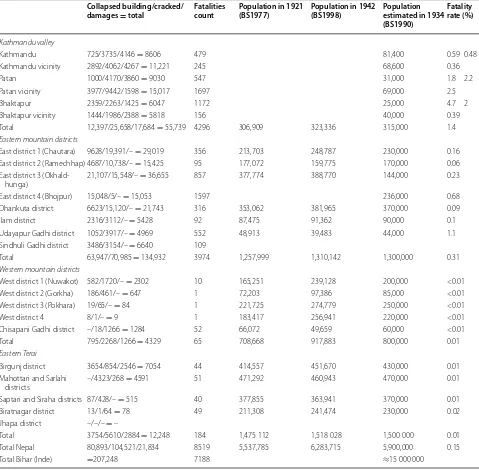
Table 1 Fatalities count per district due to the January 15, 1934, earthquake (Rana 1935) and comparison with popula-tion estimates
The population estimation in 1921 and 1942 comes from the Central Bureau of Statistics, Katmandu. The population estimation for 1934 is deduced from an extrapolation in between the values for 1921 and 1942. The population distribution in the valley in 1934 is estimated from the 1953 census (BS2009)
Collapsed building/cracked/
damages = total Fatalities count Population in 1921 (BS1977) Population in 1942 (BS1998) Population estimated in 1934 (BS1990)
Fatality rate (%)
Kathmandu valley
Kathmandu 725/3735/4146 = 8606 479 81,400 0.59 0.48
Kathmandu vicinity 2892/4062/4267 = 11,221 245 68,600 0.36
Patan 1000/4170/3860 = 9030 547 31,000 1.8 2.2
Patan vicinity 3977/9442/1598 = 15,017 1697 69,000 2.5
Bhaktapur 2359/2263/1425 = 6047 1172 25,000 4.7 2
Bhaktapur vicinity 1444/1986/2388 = 5818 156 40,000 0.39
Total 12,397/25,658/17,684 = 55,739 4296 306,909 323,336 315,000 1.4
Eastern mountain districts
East district 1 (Chautara) 9628/19,391/– = 29,019 356 213,703 248,787 230,000 0.16
East district 2 (Ramechhap) 4687/10,738/– = 15,425 95 177,072 159,775 170,000 0.06
East district 3
(Okhald-hunga) 21,107/15,548/– = 36,655 857 377,774 388,770 144,000 0.23
East district 4 (Bhojpur) 15,048/5/– = 15,053 1597 236,000 0.68
Dhankuta district 6623/15,120/– = 21,743 316 353,062 381,965 370,000 0.09
Ilam district 2316/3112/– = 5428 92 87,475 91,362 90,000 0.1
Udayapur Gadhi district 1052/3917/– = 4969 552 48,913 39,483 44,000 1.1
Sindhuli Gadhi district 3486/3154/– = 6640 109
Total 63,947/70,985 = 134,932 3974 1,257,999 1,310,142 1,300,000 0.31
Western mountain districts
West district 1 (Nuwakot) 582/1720/– = 2302 10 165,251 239,128 200,000 <0.01
West district 2 (Gorkha) 186/461/– = 647 1 72,203 97,386 85,000 <0.01
West district 3 (Pokhara) 19/65/– = 84 1 221,725 274,779 250,000 <0.01
West district 4 8/1/– = 9 1 183,417 256,941 220,000 <0.01
Chisapani Gadhi district –/18/1266 = 1284 52 66,072 49,659 60,000 <0.01
Total 795/2268/1266 = 4329 65 708,668 917,883 800,000 0.01
Eastern Terai
Birgunj district 3654/854/2546 = 7054 44 414,557 451,670 430,000 0.01
Mahottari and Sarlahi
districts –/4323/268 = 4591 51 471,292 460,943 470,000 0.01
Saptari and Siraha districts 87/428/– = 515 40 377,855 363,941 370,000 0.01
Biratnagar district 13/1/64 = 78 49 211,308 241,474 230,000 0.02
Jhapa district –/–/– = –
Total 3754/5610/2884 = 12,248 184 1,475 112 1,518 028 1,500 000 0.01
Total Nepal 80,893/104,521/21,834 8519 5,537,785 6,283,715 5,900,000 0.15
earthquakes (Szeliga et al. 2010), we retain this relation-ship in MSK-64 because it facilitates direct comparison
of our results with those of Shiono (1995).
Besides, the distribution of the collapsed buildings and fatalities are far from being as clearly related to the epi-central distance. Indeed, in the eastern districts to the south of the epicenter there are a considerable number
of collapsed buildings (see Table 2), suggesting a strong
effect of the earthquake despite a comparatively small number of victims. The effects diminish quickly eastward,
with little damage to Darjeeling (Fig. 2). To the west, in the
Kathmandu valley, the rate of victims per collapsed build-ings appears higher than elsewhere suggesting a higher vulnerability of the population to the destructions, most
probably due to the taller buildings and higher buildings density (multi-story masonry with mud cement) as well as local site conditions. These observations could therefore benefit from being confronted to demographical records.
Fatality rate collection and analysis
Besides this information on the macroseismic field, we benefited from the individual and housing counts of the Nepalese population issued before (1921) and after the earthquake (1942) by the Central Bureau of Statistics, critical information that was not available to previous
studies including Pandey and Molnar (1988). We
esti-mated the population counts in 1934 from an extrapola-tion in between the values for these censuses, estimating the average annual growth rate for each region and mak-ing the hypothesis that these rates are constant over the considered period. Given that we did not benefit from details concerning the population repartition within the Kathmandu valley in 1921 and 1942, we used those from the 1953 census, making the hypothesis that the distri-bution of the population remained similar up to at least
1953 (Table 1). The growth rate remained smaller than
1 % per year during that period; therefore, uncertainties, conservatively taken as 5 % when necessary, have no con-sequence on the conclusions we reach in this study.
We then confront, to evaluate the fatality rate, the
num-ber of victims reported by Rana (1935) to this estimate
of the 1934 population. These numbers are summarized
in Tables 1 and 2. In Kathmandu valley, the fatality rate
appears higher than in other areas of the meizoseismal zone
in Nepal (Fig. 2). Indeed, the fatality rates in Kathmandu,
Bhaktapur and Lalitpur–Patan districts are typically as high as 0.5 % or larger, while they rarely reach 0.1 % in most regions at similar distances from the epicenter. Actually, the fatality rate is of the order of 2 % for Patan, similar in and out the city center due to a mixed type of building, but var-ies in between 0.4 % for the most rural areas in Bhaktapur
-Fig. 2 Macroseismic map of the 1934 earthquake. Isoseists inter-polated from 806 MSK64 macroseismic intensities compiled in Ambraseys and Douglas (2004). Slump belt was severely affected by liquefactions and slumping (contour from Dunn et al. 1939). Red star is the instrumental epicenter of the main shock from Chen and Molnar (1977). Red polyline with triangles corresponds to the trace of the Main Frontal Thrust that ruptured in 1934 according to Sapkota et al. (2013). In gray, 1934 administrative districts borders and names. Refer to Table 1 for full district names
Table 2 Fatality rate due to the January 15, 1934, earthquake in the Kathmandu valley
The fatalities count comes from Rana (1935). The 1934 population estimate is deduced from the 1921 and 1942 census. The 2011 population is given for comparison
Area Surface (km2) Fatality rate in 1934
(%) Population esti-mated in 1934 Population density in 1934 (per km2) Population in 2011 Population density in 2011 (per km2)
Kathmandu city 49.45 0.59 81,400 1646 1,003,285 20,290
Kathmandu vicinity 345 0.36 68,600 199 696,004 2017
Kathmandu district 395 150,000 1,699,289 4302
Patan city 15.15 1.8 31,000 2046 226,728 14,970
Patan vicinity 370 2.5 69,000 187 230,878 624
Patan district 385 100,000 457,606 1189
Bhaktapur city 6.56 4.7 25,000 3810 83,658 12,753
Bhaktapur vicinity 113 0.39 40,000 356 215,046 1903
and Kathmandu to nearly 5 % for the urban community of Bhaktapur. The high fatality rate in that urban community is of the same order of magnitude as the fatality rates recorded in the worst fatal meizoseismal areas which include the cit-ies of Managua, Nicaragua, in 1972 (1 %), Spitak, Armenia, in 1988 (4.5 %), Avezzano and Messina, Italy, in 1915 and
1908 (17 and 20 %) (e.g., Nichols and Beavers 2003, 2008)
and has to be compared to the 30 % recorded in 1976 in areas of the city of Tangshan, China, exposed to total
col-lapse of masonry buildings (Shiono 1995).
This high fatality rate in Kathmandu valley is probably due to combined effects of the vulnerable multi-storys building stock, made of brick with mud mortar, its high concentra-tion and of addiconcentra-tional seismo-geological effects typical of the Kathmandu basin, including (1) very long solicitation of the structures due to trapping of the seismic waves (e.g.,
Bhatta-rai et al. 2012; Chamlagain and Gautam 2015), (2) dominant
seismic periods, related to the seismic source and sedimen-tary basin response, corresponding to the natural periods of
multi-storys buildings (e.g., Paudyal et al. 2012; Rajaure et al.
2014; Goda et al. 2015; Galetzka et al. 2015; Bhattarai et al.
2015) and (3) liquefactions (e.g., Gajurel et al. 2000; Mugnier
et al. 2011). In comparison, mountainous areas of Bhojpur
and Udaypur Gadhi fatality rates, on the hanging wall of the fault that ruptured, are of the order of one percent, which is low compared with the values observed in Kathmandu valley, but still very high for rudimentary buildings, wood-framed with light roof material, usually safer when, in addi-tion, established on the bedrock.
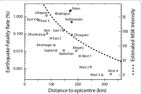
When presented as a function of the distance to
epi-center (Fig. 3), the earthquake fatality rate decreases
in a similar way as the macroseismic intensity, not tak-ing into account the most densely populated areas of the
Kathmandu valley. Indeed, those regions appear as outli-ers, far beyond average fatality rates, even when consid-ering separately the most urban areas and their vicinity
(Fig. 4). In 1934, Patan was a mix of urban and rural
envi-ronment, whereas Bhaktapur urban and rural zones were (and actually still are) very pure, an observation that help in understanding the differences between the urban and rural end members of each city. However, these fatality rates from these urban centers appear better correlated when plotted relatively to the building destruction rate
(Fig. 5), suggesting a possible causal relationship between
the fatality rate and the population density.
IX
Fig. 3 Fatality rate from the 1934 Nepal–Bihar earthquake as a function of the distance to epicenter (Rana 1935). The dashed curve
corresponds to the attenuation of the MSK macroseismic intensity from Ambraseys and Douglas (2004) as a function of the distance to epicenter. The black diamonds correspond to the samples within the Kathmandu basin
Fig. 4 Fatality rate from the 1934 Nepal–Bihar earthquake (Rana 1935) as a function of the mean MSK intensity from Ambraseys and Douglas (2004). The black diamonds correspond to the samples within the Kathmandu basin. The dashed curve corresponds to Shiono (1995) standard—unreinforced masonry—fatality rate relationship as a function of the macroseismic intensity
Fa
tality
Ra
te (%)
Building destroyed per population (/100 hab) 0.010
Fig. 5 Fatality rate from the 1934 Nepal–Bihar earthquake as a function of the building destruction (Rana 1935). The black diamonds
These fatality rates can already be used to derive first-order fatality estimates in the case of a repetition of the 1934 earthquake, assuming the local vulnerability has remained constant. For example, with the 2011 popu-lation census, we can calculate casualties in each zone used to calculate the 1934 fatality rates and reported in
Table 1. Taking into account the change in
administra-tive boundaries used in the recent census compared with 1934, we obtain numbers given in details in Additional
file 1: Table S1. We then obtain 33,000 victims in Nepal,
but over 50,000 in India. Due to the large increase in population in northern India, larger numbers of victims are expected in India, while the rupture zone remains in Nepal. If the 2001 census population is used instead, we obtain about 26,000 victims in Nepal and 39,000 in India. An interesting temporal variability can be observed when the 2001 and 2011 censuses are compared, beyond just the unavoidable increase in the number of victims. Popu-lation growth remains larger than 20 % per year in India, but is decreasing to values of the order of 14 % in Nepal. Hill districts of the epicentral zone of the 1934 earth-quake tend to lose population, while Nepalese population dramatically increases in the foothills near the Indian border. Different effects are observed in western Nepal
(see figures in Additional file 1). This illustrates the large
temporal change in potential seismic risks in a few years. The numbers of victims estimated above can only be considered as a baseline. Indeed, numerous effects com-plicate the problem. In addition to the population growth and redistribution, the fatality rates must have been mod-ified by the change in population lifetime and the evolu-tion of construcevolu-tion methods. The April 25, 2015, Gorkha earthquake definitely brings important new information to address these problems.
Comparison with the 2015 Gorkha earthquake
The earthquake of April 25, 2015 (Fig. 1), of magnitude
Mw ~7.8 (ML ~7.6), with more than 8700 victims, is the
most deadly earthquake in Nepal since the Mw ~8.4
meg-aquake of 1934. Beyond the large number of victims, the destruction of infrastructure and houses was tremendous in the villages north of Kathmandu, even total in some locations, and a terribly traumatic situation was cre-ated for the population. While the epicenter was loccre-ated near Gorkha city, the aftershock distributions covered a 150-km segment extending to the east (Adhikari et al.
2015). Fatality rates were moderate in the Katmandu
Val-ley (<0.1 %), but was surprisingly large in hill districts north of Kathmandu, with a maximum fatality of 1.5 % in Rasuwa District, 1.2 % in Sindhupalchowk district and 0.4 % in Nuwakot district (Central Department of Statis-tics, Home Ministry, Nepal). When comparing the fatal-ity rate with the building destruction rate per inhabitant
(Fig. 5), the fatalities of the Gorkha earthquake appear
significantly smaller than for the 1934 earthquake, while the building destruction rate appears comparatively large for the 2015 Gorkha earthquake. Actually, in some rural communities north of Kathmandu, the building destruc-tion rate was close to 100 % in 2015. This suggests that large differences in some rural and some urban districts have now emerged in Nepal, with the implementation of appreciably efficient building methods in Kathmandu val-ley, while the construction methods were not improved at all since the 1934 earthquake in rural communities. Note that the 1934 and 2015 earthquakes both happened on a holiday around noon time.
The intensity distribution in the case of the Gorkha
earthquake (Martin et al. 2015) hardly compares with
predictions from known attenuation laws of the mac-roseismic intensity at short distance (the first tenths of kilometers) from the source. Nevertheless, to compare with the previous analysis for the 1934 earthquake, we
use again the Ambraseys and Douglas (2004)
attenua-tion law to estimate the intensities, taking into account an effective macroseismic epicenter north of Kath-mandu in the center of the aftershock distribution. We note that the macroseismic intensities predicted by this attenuation law are significantly larger than what was
observed for the Kathmandu valley (Martin et al. 2015),
10 to 30 km from the ruptured fault segment (e.g.,
Avouac et al. 2015; Grandin et al. 2015; Kobayashi et al.
2015). The fatality rates versus the estimated
intensi-ties (Fig. 6) are significantly smaller than the values
Fa
observed for the 1934 earthquake. This conclusion still hold after converting the estimated intensities in true intensities at observation sites documented both in 1934
and 2015, respectively, in Martin and Szeliga (2010) and
Martin et al. (2015). In Fig. 6, scaling laws proposed by
Shiono (1995) are also shown versus intensity. While the
large heterogeneity mentioned before causes large scat-ter in the case of the Gorkha earthquake (e.g., intensi-ties reported in Kathmandu valley typically range from
IEMS98 6 to 8), the so-called composite building Shiono
scaling law appears on average as a satisfactory descrip-tion of the 2015 data.
Conclusions
In this paper, complementing previously known informa-tion, the censuses carried out in 1921 and 1942 in Nepal are used to evaluate the fatality rates from the great 1934 Bihar–Nepal earthquake and better characterize its impact in eastern Nepal. Such data provide important archives, given the scarcity of documented magnitude 8 earthquakes. While rarely exceeding 1 %, even in the most impacted areas of eastern Nepal, close to the epi-center and on the hanging wall of the thrust fault that was activated, the fatality rates exceed 0.5 % in Kathmandu valley, reaching even 5 % in urban Bhaktapur. Such observed fatality rates can be used to broadly estimate their order of magnitude in case this earthquake repeats. While the numbers obtained have to be taken with cau-tion, they definitely illustrate that the country has to con-sider preparations. The order of magnitude of temporal
variations (+15 % per decade) noted when using 2001 or
2011 population numbers, and the fact that larger num-bers of victims have now to be expected on the India side, are probably robust.
Compared with the fatality rates of the 1934 earth-quake, the fatalities of the 2015 earthquake are signifi-cantly smaller for a given estimated intensity, except in some hill districts. This suggests that the lessons of the 1934 earthquake may have been ignored in some rural districts and that earthquake prevention methods have not been widely implemented outside the Kathmandu valley. This is also illustrated by the fact that the
compos-ite Shiono scaling law (Shiono 1995), which reflects the
building prevention strategies suggested in Asia after the 1976 Tangshan earthquake in China, appears to repro-duce, on average, the 2015 fatality rates, while the scal-ing law for unreinforced masonry reproduces the 1934 earthquake. Therefore, while numerous problems remain open, the results of decades of earthquake prevention methods, indeed, seem to have saved a significant num-ber of lives in 2015. In the absence of more precise work, the composite Shiono scaling law could be a reasonable
approach to estimating casualties in the case of contem-porary large Himalayan earthquakes.
While simple scaling laws, in no way, can be claimed as reliable predictive models, they suggest important fea-tures that can be used to guide further research. In any case, given the large increase in population crowding in buildings, which are built both in Nepal and in India without much consideration for earthquake hazards (e.g.,
Dixit et al. 2013), it is the duty of the scientific
commu-nity to raise great concern in this matter, and to make sure that every possible steps are taken to mitigate the effects of the coming megaquake in the Himalayan foot-hills. Intensity and fatality distributions from the 2015 Gorkha earthquake, while referring to a smaller earth-quake and probably of a different kind, will be of tre-mendous importance to better constrain possible fatality scaling laws, and the potential damage and loss of life from the next giant Himalayan earthquake.
Authors’ contributions
The material of this paper is part of the doctoral thesis of SNS, defended in 2011 at IPGP. All three authors contributed to the data analysis and manu-script. All authors read and approved the final manumanu-script.
Author details
1 Department of Mines and Geology, Lainchaur, Kathmandu, Nepal. 2 Départe-ment Analyse et Surveillance EnvironneDéparte-ment, CEA, DAM, DIF, 91297 Arpajon, France. 3 Institut de Physique du Globe de Paris, Sorbonne Paris Cité, Université Paris Diderot, CNRS, 75005 Paris, France.
Acknowledgements
We would like to thank the Central Bureau of Statistics, Katmandu, for provid-ing the census records. We also thank DASE-France and the Department of Mines and Geology, Kathmandu, Nepal, for constant support. We appreciated discussions with Paul Tapponnier and the feedback from two reviewers. This is IPGP contribution 3710.
Competing interests
The authors declare that they have no competing interests.
Received: 10 September 2015 Accepted: 11 February 2016
Additional file
Additional file 1: Text S1. Biography of Brahma Shamsher Rana (December 1909–January 1989) Personal communicationwith Sagar Shamsher Janga Bahadur Rana (Nephew of Brahma Shamsher). Table S1.
Fatalities count per district due to a repetition of the January 15th, 1934 earthquake in 2001 and in 2011, applying the fatality rates observed in 1934. The population is the divisions used in 1934 are estimated using the 2001 and 2011 census data (Central Bureau of Statistics). Table S2. District name equivalence between Rana (1935) and present-day districts names.
Figure S1. Map of eastern nepal districts showing an estimate of the population derived from 1921 and 1942 census (green in thousands), the number of fatalities (red) (and the number of collapsed buildings (violet) (Rana, 1935). Figure S2. Map of the fatality rates (this study) and damages mentioned in Rana 1935. MSK VIII isoseist from this study. Figure S3.
Population distribution in 2011 according to the 2011 Census. Figure S4.
References
Adhikari LB, Gautam UP, Koirala BP, Bhattarai M, Kandel T, Gupta RM, Timsina C, Maharjan N, Maharjan K, Dahal T, Hoste-Colomer R, Cano Y, Dandine M, Bollinger L (2015) The aftershock sequence of the April 25 1 2015 Gorkha-Nepal earthquake. Geophys J Int 203:2119–2124
Ambraseys NN, Douglas J (2004) Magnitude calibration of north Indian earth-quakes. Geophys J Int 159:165–206
Avouac JP, Meng L, Wei S, Wang T, Ampuero JP (2015) Lower edge of locked Main Himalayan Thrust unzipped by the 2015 Gorkha earthquake. Nat Geosci 8(9):708–711
Bhattarai M, Gautam U, Pandey R, Bollinger L, Hernandez B, Boutin V (2012) Capturing first records at the Nepal NSC accelerometric network. J Nepal Geol Soc 43:15–22
Bhattarai M, Adhikari LB, Gautam UP, Laurendeau A, Labonne C, Hoste-Colomer A, Sèbe O, Hernandez B (2015) Overview of the large April 25th 2015 Gorkha, Nepal earthquake from accelerometric perspectives. Seism Res Lett 86(6):1540–1548. doi:10.1785/0220150140
Bilham R (2004) Urban earthquake fatalities: a safer world, or worse to come? Seismol Res Lett 75:706–712
Bilham R (2009) The seismic future of cities. Twelfth Annual Mallet-Milne Lec-ture. Bull Earthquake Eng 2009:1–49. doi:10.1007/s10518-009-9147-0 Bilham R, Blume F, Bendick R, Gaur VK (1998) Geodetic constraints on the
translation and deformation of India: implications for future great Himala-yan earthquakes. Curr Sci 74(3):213–229
Bollinger L, Sapkota SN, Tapponnier P, Klinger Y, Rizza M, Van der Woerd J, Tiwari DR, Pandey R, Bitri A, Bes de Berc S (2014) Estimating the return times of great Himalayan earthquakes in eastern Nepal: evidence from the Patu and Bardibas strands of the Main Frontal Thrust. J Geophys Res. doi:10.10 02/2014JB010970
Chamlagain D, Gautam D (2015) Seismic hazard in the Himalayan inter-montane basins: an example from Kathmandu Valley, Nepal. In: Shaw R, Nibanupudi HK (eds) Mountain hazards and disaster risk reduction. Springer, Japan, pp 73–103
Chen WP, Molnar P (1977) Seismic moments of major earthquakes and the average rate of slip in Central Asia. J Geophys Res 82:2945–2969 Dixit AM, Yatabe R, Dahal RK, Bhandary NP (2013) Initiatives for earthquake
dis-aster risk management in the Kathmandu Valley. Nat Hazards 69:631–654 Dunn JA, Auden JB, Gosh AMH, Roy SC, Wadia DN (1939) The Bihar–Nepal
earthquake of 1934, vol 73. Memoirs of the geological survey of India, Geological Survey of India
Gajurel AP, Huyghe P, Upreti BN, Mugnier JL (2000) Palaeoseismicity in the Koteshwor area of the Kathmandu valley, Nepal, inferred from the soft sediment deformational structures. J Nepal Geol Soc 22:547–556 Galetzka J, Melgar D, Genrich JF, Geng J, Owen S, Lindsey EO, Xu X, Bock Y,
Avouac J-P, Adhikari LB, Upreti BN, Pratt-Sitaula B, Bhattarai TN, Sitaula BP, Moore A, Hudnut KW, Szeliga W, Normandeau J, Fend M, Flouzat M, Bollinger L, Shrestha P, Koirala B, Gautam U, Bhatterai M, Gupta R, Kandel T, Timsina C, Sapkota SN, Rajaure S, Maharjan N (2015) Slip pulse and resonance of the Kathmandu basin during the 2015 Gorkha earthquake, Nepal. Science 349(6252):1091–1095. doi:10.1126/science.aac6383 Goda K, Kiyota T, Pokhrel R, Chiaro G, Katagiri T, Sharma K, Wilkinson S (2015)
The 2015 Gorkha Nepal earthquake: insights from earthquake damage survey. Front Built Environ 1(8):2015. doi:10.3389/fbuil.2015.00008 Grandin R, Vallée M, Satriano C, Lacassin R, Klinger Y, Simoes M, Bollinger L
(2015) Rupture process of the Mw= 7.9 Gorkha earthquake (Nepal): insights into Himalayan megathrust segmentation. Geophys Res Lett 42(20):8373–8382
Hough SE, Bilham R (2008) Site response of the Ganges basin inferred from re-evaluated macroseismic observations from the 1897 Shillong, 1905 Kangra, and 1934 Nepal earthquakes. J Earth System Sci 117(S2):773–782 Jackson J (2006) Fatal attraction: living with earthquakes, the growth of
vil-lages into megacities, and earthquake vulnerability in the modern world. Phil Trans R Soc A 364:1911–1925
Kobayashi T, Morishita Y, Yarai H (2015) Detailed crustal deformation and fault rupture of the 2015 Gorkha earthquake, Nepal, revealed from ScanSAR-based interferograms of ALOS-2. Earth Planets Space 67:201
Maqsood ST, Schwarz J (2011) Estimation of Human casualties from earthquakes in Pakistan—an engineering approach. Seismol Res Lett 82(1):32–41. doi:10.1785/gssrl.82.1.32
Martin S, Szeliga W (2010) A catalog of felt intensity data for 570 earthquakes in India from 1636 to 2009. Bull Seismol Soc Am 100(2):562–569 Martin SS, Hough SE, Hung C (2015) Ground motions from the 2015 Mw 7.8
Gorkha, Nepal, earthquake constrained by a detailed assessment of macroseismic data. Seismol Res Lett 86(6):1524–1532
Middlemiss CS (1910) The Kangra earthquake of 4th April, 1905. Geol Surv India Mem 37:1–409
Mugnier JL, Huyghe P, Gajurel AP, Upreti BN, Jouanne F (2011) Seismites in the Kathmandu basin and seismic hazard in central Himalaya. Tectonophysics 509(1–2):33–49
Nichols JM, Beavers JE (2003) Development and calibration of an earthquake fatality function. Earthquake Spectra 19(3):605–633
Nichols JM, Beavers JE (2008) World earthquake fatalities from the past: impli-cations for the present and future. Nat Hazards Rev 9:179–189 Oldham RD (1899). Report on the great earthquake of 12th June 1897.
Mem-oirs of the Geological Survey of India, pp 1–379
Pandey MR, Molnar P (1988) The distribution of Intensity of the Bihar Nepal earthquake of 15 January 1934 and bounds on the extent of the rupture. J Nepal Geol Soc 5:22–44
Paudyal YR, Bhandary NP, Yatabe R (2012) Seismic microzonation of densely populated area of Kathmandu valley of Nepal using microtremor obser-vations. J Earthquake Eng 16:1208–1229
Pulla P (2015) New jitters over megaquakes in Himalayas. Science 347(6225):933–934
Rajaure S, Koirala B, Pandey R, Timsina C, Jha M, Bhattarai M, Dhital MR, Paudel LP, Bijukchhen S (2014) Ground response of the Kathmandu Sedimentary Basin with reference to 30 August 2013 South-Tibet Earthquake. J Nepal Geol Soc 47:23–34
Rajendran CP, Biju J, Rajendran K (2015) Medieval pulse of great earthquakes in the central Himalaya: viewing past activities on the frontal thrust. J Geophys Res 123:1623–1641
Rana BS (1935) Nepal Ko Maha Bhukampa (The great earthquake of Nepal). Jorganesh Press, Kathmandu, pp 1–250 (in nepali)
Sapkota SN, Bollinger L, Klinger Y, Tapponnier P, Gaudemer Y, Tiwari DR (2013) Primary surface ruptures of the great Himalayan earthquakes in 1934 and 1255. Nat Geosci 6:71–76
Shiono K (1995) Interpretation of published data of the 1976 Tangshan, China Earthquake for the determination of a fatality rate function. Japan Soc Civil Eng Struct Eng Earthquake Eng 11(4):155s–163s