Automatic Classification Of Stock Twitter Data
By Using Different Svm Kernel Functions
Lakshmana Phaneendra Maguluri, R Ragupathy
Abstract: Twitter is an American online microblogging and social networking platform where people around different places of the world share their opinions, express their views on various topics, discuss current issues and etc. These opinions and reviews which are seen on this platform are based on that particular individual’s perspective which can be conflicting to others. Also, the numbers of reviews on this platform are so many that one cannot go through all those reviews to come to a conclusion about what they are searching for. In order to perform this analysis, we take the help of Twitter UPI, a major source that is used for the collection of a dataset and real-time tweets and performs analysis on that data. In this paper, the emotional tone behind a series of words on twitter is determined. The main objective is to implement various algorithms like Support Vector Machine (SVM) and Naïve Bayes (NB) for the classification of tweets. The approach followed here primarily focuses on the real-time analysis and classifies the polarity of a tweet at the word level and each tweet is categorized is either positive or negative with help of feature vector and classifiers of the above algorithms. Also quantitative analysis of SVM and NB are carried out through performance metrics like accuracy, sensitivity, specificity, prevalence, kappa, etc.
Index Terms: Microblogging, Machine Learning Algorithms, Performance Metrics, Social Media, Sentiment Analysis. —————————— ——————————
1.
INTRODUCTION
Nowadays all of the big companies try to understand the sentiment of their customers. They try to analyze what are the customers toking about, how they are saying it, and what they exactly mean by it. So, Sentiment analysis is basically a particular domain where you try to understand human emotions with software. If these human emotions are in written form, we can go ahead and classify these sentiments to positive, negative or neutral. Sometimes Opinion mining referred as Sentiment analysis because what we are basically doing is, trying to figure out the Opinion or the attitude of the customer with respect to a Tweet. So, now we`ll go ahead and look and look at some interesting applications of Sentiment Analysis. So, Sentiment Analysis can be used for review classification, product review mining and also during election times. In the past decade also there has huge increase in online activity across the globe. So, every single second, people make millions of tweets and this is where social media plays a pivotal role. Now social media is not just any other platform. People go on to Social media and express their views in the form of tweets. They tweet about their likes and their dislikes. There is where we are able to tap all these tweets, it can be very useful to us to know about the sentiment or Opinion of people mindset of Current Scenario. So today we`re going to do a bit of Twitter Sentiment Analysis. Twitter sentiment analysis has become the talk of the town when people got curious about the sentiment analysis of the posted tweets. Microblogging is a very small blogging and the most popular way of microblogging nowadays is through Twitter that allows users to post tweets, which can be 140 character messages, videos, photos or links. Twitter has become a staple much like Facebook and teens are big users.
All age category people around the world exchange their views, express opinions in the twitter platform. All those who register on this platform can view and post tweets and can interact with various kinds of people whereas unregistered people can only view tweets but cannot post any tweets on this particular platform. Twitter has more than 336 million monthly active users until the end of January 2019. Sentimental analysis of twitter-based tweets can be further classified into three different categories Emoticon, Polarity, and Strength. When we are extracting emotions expressed in tweets which are having some values for every facial expression. Basically polarity values can be extracted from the tweeted sentence and these values can be classified as +ve, -ve or neutral. Lastly in strength-based analysis information from tweets is extracted and we will assign an equivalent numerical value for different tweets or sentences with respect to the intensity of tweet returned.
2
RELATED
WORK
In 2009, Alec G et al [8] introducing a novel approach for automatic classification of Tweets Based on the query term Tweets can be automatically classified into positive or negative classes. By using a different machine learning Algorithms with different feature extractions techniques, unigrams, bigrams, and POS to achieve high accuracy. In 2011, Apoorv Agarwal et al [9] designed an approach for sentiment analysis of Twitter Data. He combined tree kernel and feature-based models to perform classification of Tweets basically into 3 categories of classes ―+ve‖, ―-ve‖ and ―neutral‖. These models outperform the unigram baseline. To perform feature extraction, he combines both prior polarities of words and their POS. In 2014, Walaa Medhat et al [5] written Sentiment Analysis Algorithms and Applications: A Survey. This survey’s main target is to give a clear picture of sentiment analysis techniques in brief. So, that researcher can quick start the research in a recent trend in the era of sentiment analysis. _____________________________
Lakshmana phaneendra maguluri, Department of Computer Science and Engineering, Annamalai University, Annamalai Nagar, Chidambaram, Tamil Nadu, India-608002, PH-9666966077. E-mail: [email protected]
In 2016, M.Kiruthika et al [2] has been carried out Sentiment Analysis of Tweet by using an aspect level-based approach for sentiment classification. They proposed a system that would analyze tweets about movies into three categories as it is desirable to understand the sentiment of each aspect of different entities for deep grained analysis. In 2016, Akshay Amolik et al [1] in this paper with the help feature vector and machine learning classifier developed Twitter Sentiment Analysis of latest movie reviews using Machine learning techniques. 75% accuracy from SVM, 65% accuracy from NB are the results obtained by implementing machine learning techniques. They also concluded that the accuracy of classification can be increased by increasing the training data. In 2017, Shubham S. Deshmukh et al [6] had given design and implementation of Twitter Data Analysis and Visualization in R platform for Twitter data. This primarily focuses on real-time analysis rather than historic datasets.
3 MACHINE
LEARNING
ALGORITHMS
In this paper we take the help of SVM and NB algorithms for automatic classification of tweets [7]. Finding whether the expressed opinion is positive or negative i.e., classifying the polarity of a given tweet is our main concern and problem statement of twitter sentiment analysis. We computationally identify and categorize Sentiment expressed in a tweet, in order to determine whether the Customer or user mindset towards a particular Scenario or product is positive, negative or neutral.
3.1 Naïve Bayes Theorem
Understanding Naïve Bayes and machine learning like with any of our other machine learning tools it’s important to understand where the Naïve Bayes fits in the hierarchy. So under Machine Learning, we have Supervised Learning and there are other things like unsupervised Learning, this falls under the supervised learning and under the supervised learning there`s classification and there`s also a regression but we are going to be in classification side and under the classification side Naïve Bayes Classifier. As a Classifier we use in face recognition, weather prediction, Medical Diagnosis and News Classification. The probability value by which Naïve Bayes classifier works predicted as shown in (1)
𝑝(𝑓) = (𝑝(𝑙) ∗ 𝑝(𝑓/𝑙))/(𝑝(𝑓)) (1)
Where,
P (l) is the prior probability of a label.
P (f | l) is the prior probability that a given feature set is being classified as a label.
P (f) is the prior probability that a given feature set is occurred.
Given the Naïve assumption which states all features are independent, the equation could be rewritten in (2).
𝑝(𝑓) = (𝑝(𝑙) ∗ 𝑝(𝑓1/𝑙) ∗ … . .∗ 𝑝(𝑓𝑛/𝑙))/(𝑝(𝑓𝑠)) (2)
Where,
P (fs) is equal to P (features), P (l) is equal to P (label).
In analysis, each feature is independent which the advantage of NB classifier.
Another major advantage of NB classification is easy to
interpret and computation is efficient. 3.2 . Support Vector Machine
The SVM is basically is a classifier that separates that data into different classes based on their membership, with the help of a hyper plane. This SVM makes use of the different type of kernels based on the requirement for the computation. It can be used as both classification and regression model. The input set of data are usually vector and are later classified into classes. Once we have the data, we need to draw a decision boundary which is called a hyperplane anywhere between the two classes. To get a precise location of the decision boundary, because if we get that line incorrect we cannot precisely classify the data. So we draw two more decision lines using our intuition and calculate the precise location of the decision boundary. The above mentioned process is given in the below, Fig.1.
Fig.1. Support Vector Machine
From Fig.1, H1, H2 & H3 are the support vectors. Here we need to check the maximum margin from the two classes and consider it as a hyperplane. H1 has no scope of separating the classes, coming to H2 it has small margin length from the classes and H3 which is possessing the maximum margin Length and can be considered as the hyperplane. The SVM has a function called descriptive which is shown in (3)
(𝑥) = 𝑧 ∅(𝑥) + 𝑐 (3)
Where X is called as the feature vector, the different weights are represented by z, the Ø used to represent the non-linear mapping function and bias vector is denoted by c. Here the weights and the bias vector are learning from the data set provided.
3.3 Kernels in Support Vector Machine
The SVM’s uses certain kind of functions called kernel to compute the data and change it into required form. There are many kernel functions available but the most significant ones are given below.
Significant kernels used in SVM are, 1. Polynomial
4. Sigmoid
Polynomial Kernel: This is a kernel function used in the support vector machine and also in the many other models that makes use of the kernel functions. The polynomial kernel is used to represent the similarities between the vectors (training examples) over the polynomials of the original variable and all this process computes in the feature space and helps us to learn about the non-linear models. Radial Kernel: This radial kernel is also called as Radial Basis Function (RBF). This type of kernel is basically used in the support vector machine classification. And also the Euclidean distance between the two feature vectors may be calculated as squared. Linear Kernel: Of all available kernels this linear kernel considered to be extremely fast data mining algorithm. It is also the one with high accuracy rate and performance. Usually when the given data can be separated by one line, this linear kernel is used in SVM. And also preferably it is used on ultra large datasets. Sigmoid Kernel: A SVM which is making use of this kernel function is similar to the two-layer perceptron neural network, as this kernel is taken from the neural networks only when the activation function comes from the bipolar sigmoid function. SVM can also be used for the high end binary classification. The SVM can exhibits an effective performance in the high dimensional feature space. The best algorithm to use when the classes are separable to classify.
4
PROPOSED
SYSTEM
4.1 Existing System
One of the existing system contains the following modules, 1. Data Collection using Twitter API
2. Data Pre-processing
3. Applying Classification Algorithms 4. Classified Tweets
5. Sentiments in graphical representation.
Data Collection Using Twitter API: Large datasets are not available publically to the users to take from the Twitter, so the system first makes sure that the data is extracted from the Twitter API. Data Pre-Processing: The extracted data can’t be without any error. So here we process the data and make it error free and simplify the data. The operations like spell
correction, punctuation marking, etc. Applying Classification Algorithms: Here we categorize the data (tweets) into different types by using the classification algorithms. It’s also preferable to use the algorithm that provides us with high accuracy. Classified Tweets: The tweets available in the Twitter API are comprised of different categories like positive, negative or neutral and the results are taken from the above step. Sentiments in Graphical Representation: In here we make use of pie charts to display the result obtained in the sentiment analysis.
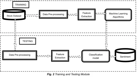
4.2 Proposed System
Fig. 2 Training and Testing Module
Fig.3 Real – Time Implementation Module
5 EXPERIMENTAL
RESULTS
AND
DISCUSSION
5.1 Datasets
The collected datasets area unit analyzing the information to go looking the sentiment on Twitter [3], some of the twitter datasets area unit that is that the most closely fits for carrying for work and seventieth of train data and the rest half-hour of the check knowledge into consideration in analyzing the
sentiment. Seventieth of train knowledge and therefore the rest half-hour of check knowledge area unit taken into consideration in analyzing the sentiment. The collected datasets area unit
(i)
https://old.datahub.io/dataset/twitter-sentiment-analysis
(ii)
https://github.com/vineetdhanawat/twitter-Stock Dataset Data Pre-processing
Feature Extraction
Machine Learning Algorithms TRAINING
Data Pre-processing Feature
Extraction
Classification
model Sentiment
TESTING
Stock Dataset Data Pre-processing Feature Extraction
Machine Learning Algorithms TRAINING
Data Pre-processing Extraction Feature Classification model Sentiment
sentimentanalysis/blob/master/datasets/Sentimen t Analysis Dataset.csv
(iii) https://data.world/crowdflower/airline-twitter
sentiment
This paper used the dataset out there in
―https://github.com/vineetdhanawat/twitter-sentiment-analysis/blob/master/datasets/Sentiment AnalysisDataset.csv‖. It contains 3 columns, particularly Id No, Sentiment, Tweets regarding 1048588 tweets. The column ―sentiment‖ can offer the particular sentiment that lies behind every tweet. In Order to coach the machine once the dataset is downloaded and pre-processing followed by the feature extraction and MLA modules area unit disbursed. Then the work thought of all the data alongside the size of 100counts of tweets, i.e.100, 200... Till 1048588.The conniving numerous metrics performances area unit created in line chat with all the parameters [4]. In SVM, in every coaching, with completely different kernels, tweets area unit from one hundred to one hundred thousand and individual kernel’s performance metrics area unit found. In every one of the on top of mentioned case, a line chart is drawn that would illustrate the parameters like accuracy, sensitivity, specificity, prevalence, detection rate, detection prevalence, precision, etc.
5.2 Performance Metrics
An application developer can create as many number of applications and a result of confusion matrix which is in the form of 2x2 Matrices. The 2x2 matrices are True Positive (TP), True Negative (TN, False Positive (FP), and False Negative (FN). From this one we can calculate the performance metrics like accuracy, specificity, sensitivity, etc. As the testing is done easily then classified model is sentiment could be obtained. There are various performance measures that are in order to know how the machine learning works, that are obtained from Metrix like confusion matrix given in table 3.Instead of calculating an error between predicted values and known values in classification, the actual predict value can compare directly with the help of confusion matrix then the Metrix will contrast predictions to the actual results. The both results are TP and TN are found along with the diagonal. All other cells are indicate the false results, i.e. FN and FP. Here Actual can also be referred as Reference.
TABLE 1CONFUSION MATRIX
Predicted
Actual
Negative Positive
Negative TN FP
Positive FN TP
From Table 1, leading diagonals are the cells that carry truly predicted, i.e. actual and predicted lies the same whereas the rest gives false values. From the Confusion Matrix, some of the metrics like Sensitivity, Specificity, Kappa, Prevalence, Detection Rate, Detection Prevalence, Balance, Accuracy (ACC), Precision (PREC), Recall (REC), F – Measure (FM), True Positive Rate (TPR), False Positive Rage (FPR), Positive predictive value (PPV), negative predictive value (NPV), etc. Following equations give a brief idea of how all the above measures could be calculated from the Confusion Matrix. Accuracy: The proportion of the whole variety of predictions is given by atomic weight by. (4)
𝐴𝑐𝑐𝑢𝑟𝑎𝑐𝑦 % = (("𝑇𝑁 + 𝑇𝑃"))/ (("𝑇𝑁 + 𝐹𝑁 + 𝐹𝑃 + 𝑇𝑃”)) (4)
Precision: The proportion of the predicted relevant materials, dataset is given by. (5)
𝑃𝑟𝑒𝑐𝑖𝑠𝑖𝑜𝑛 % = 𝑇𝑃/ ((𝐹𝑃 + 𝑇𝑃)) (5)
Recall: The proportion of the relevant materials, dataset identified from. (6)
𝑅𝑒𝑐𝑎𝑙𝑙 % = 𝑇𝑃/((𝐹 + 𝑇𝑃) ) (6)
F – Measure: Derives from precision and recall values mentioned in. (7)
𝐹 − 𝑚𝑒𝑎𝑠𝑢𝑟𝑒 % = ((2 𝑥 𝑅𝐸𝐶 𝑥 𝑃𝑅𝐸𝐶) )/((𝑅𝐸𝐶
+ 𝑃𝑅𝐸𝐶) ) (7)
True Positive Rate: TPR measures the number of relevant tuples, is given by. (8)
𝑇𝑃𝑅 = 𝑇𝑃/((𝑇𝑃 + 𝐹𝑁) ) (8)
False Positive Rate: FPR measures the number of incorrect classifications of relevant tuples out of irrelevant test tuples mentioned in. (9)
𝐹𝑃𝑅 = 𝐹𝑃/((𝐹𝑃 + 𝑇𝑁) ) (9)
Positive Predictive Value: In this positive value is equivalent to precision where the classes are perfectly balanced and it's very similar to precision and expert s that takes prevalence into account as shown in. (10)
𝑃𝑃𝑉 = ((𝑠𝑒𝑛𝑠𝑖𝑡𝑖𝑣𝑖𝑡𝑦 ∗ 𝑝𝑟𝑒𝑣𝑎𝑙𝑒𝑛𝑐𝑒))/(((𝑠𝑒𝑛𝑠𝑖𝑡𝑖𝑣𝑖𝑡𝑦 ∗ 𝑃𝑟𝑒𝑣𝑎𝑙𝑒𝑛𝑐𝑒) + (1 − 𝑠𝑝𝑒𝑐𝑖𝑓𝑖𝑐𝑖𝑡𝑦) ∗ (1 − 𝑃𝑟𝑒𝑣𝑎𝑙𝑒𝑛𝑐𝑒))) (10)
Negative Predictive Value: NPV is given by. (11)
𝑁𝑃𝑉 = ((𝑠𝑝𝑒𝑐𝑖𝑓𝑖𝑐𝑖𝑡𝑦 ∗ (1 − 𝑝𝑟𝑒𝑣𝑎𝑙𝑒𝑛𝑐𝑒)))/((((1 − 𝑠𝑒𝑛𝑠𝑖𝑡𝑖𝑣𝑖𝑡𝑦) ∗ 𝑃𝑟𝑒𝑣𝑎𝑙𝑒𝑛𝑐𝑒) + ((𝑠𝑝𝑒𝑐𝑖𝑓𝑖𝑐𝑖𝑡𝑦) ∗ (1
− 𝑃𝑟𝑒𝑣𝑎𝑙𝑒𝑛𝑐𝑒)))) (11)
Kappa: This is primarily a live off however well the classifier performed as compared to however well it might have performed just by likelihood. In different words, a model can have a high letter of the alphabet score if there's a giant distinction between the accuracy and also the null error rate. Sensitivity and Specificity: Both are statistical measures of the performance of a binary classification test is given in. (12) and (13)
𝑠𝑒𝑛𝑠𝑖𝑡𝑖𝑣𝑖𝑡𝑦 = (𝑛𝑢𝑚𝑏𝑒𝑟 𝑜𝑓 𝑡𝑟𝑢𝑒 𝑝𝑜𝑠𝑖𝑡𝑖𝑣𝑒𝑠) /(𝑛𝑢𝑚𝑏𝑒𝑟 𝑜𝑓 𝑡𝑟𝑢𝑒 𝑝𝑜𝑠𝑖𝑡𝑖𝑣𝑒𝑠
𝑠𝑝𝑒𝑐𝑖𝑓𝑖𝑐𝑖𝑡𝑦 = (𝑛𝑢𝑚𝑏𝑒𝑟 𝑜𝑓 𝑡𝑟𝑢𝑒 𝑛𝑒𝑔𝑎𝑡𝑖𝑣𝑒𝑠) /(𝑛𝑢𝑚𝑏𝑒𝑟 𝑜𝑓 𝑡𝑟𝑢𝑒 𝑛𝑒𝑔𝑎𝑡𝑖𝑣𝑒𝑠
+ 𝑛𝑢𝑚𝑏𝑒𝑟 𝑜𝑓 𝑓𝑎𝑙𝑠𝑒 𝑝𝑜𝑠𝑖𝑡𝑖𝑣𝑒𝑠) (13)
In pattern recognition and information retrieval is given in. (14) and (15)
𝑝𝑟𝑒𝑐𝑖𝑠𝑖𝑜𝑛 = (|*𝑟𝑒𝑙𝑒𝑣𝑎𝑛𝑡 𝑑𝑜𝑐𝑢𝑚𝑒𝑛𝑡𝑠+ ∩ *𝑟𝑒𝑡𝑟𝑖𝑒𝑣𝑒𝑑 𝑑𝑜𝑐𝑢𝑚𝑒𝑛𝑡𝑠+|)
/(|*𝑟𝑒𝑡𝑟𝑖𝑒𝑣𝑒𝑑 𝑑𝑜𝑐𝑢𝑚𝑒𝑛𝑡𝑠+|) (14)
𝑟𝑒𝑐𝑎𝑙𝑙 = (*𝑟𝑒𝑙𝑒𝑣𝑎𝑛𝑡 𝑑𝑜𝑐𝑢𝑚𝑒𝑛𝑡𝑠+ ∩ *𝑟𝑒𝑡𝑟𝑖𝑒𝑣𝑒𝑑 𝑑𝑜𝑐𝑢𝑚𝑒𝑛𝑡𝑠+|)
/(|*𝑟𝑒𝑡𝑟𝑖𝑒𝑣𝑒𝑑 𝑑𝑜𝑐𝑢𝑚𝑒𝑛𝑡𝑠+|) (15)
Null Error Rate: Null error rate are often helpful for baseline metric to match the simplest classifier for a selected application can typically have the best error rate than the null error rate.
5.3 Results and Discussion
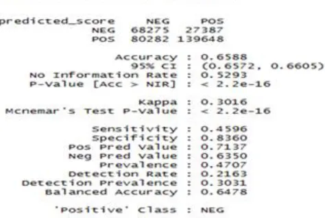
Performance Metrics For 1048588 Tweets in NB and SVM: For each sale of the tweets count then calculate all the metrics performances with the help of confusion matrix as given below table 3,various performance metrics discussed it can be calculated.
Fig. 5 - Performance Metrics of 1048588 tweets in Naïve Bayes
Null error gives for all under NB tweets performance metrics, similar kind of Metrics performance can be calculated for various kernels in SVM. The paper proposed some of the results were made with the help of stored CSV files that are discussedCSV File Format for all 1048588 Tweets in NB and SVM: By the means of sampling dataset under the SVM and NB, are separate files are stored in the form of comma separated value file. Naive Bayes with the performance metrics on different scales of tweets which are given in csv file format is given in fig.6
Fig. 6 CSV File Format for 1048588 tweets in Naïve Bayes and its metrics
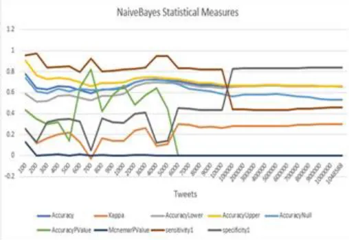
Above NB CSV file, separate csv files may be generated for all the kernels of SVM. Naïve Bayes and its Performance Metrics: Under Naïve Bayes, the paper, thought of all 1048588 tweets along within the scales of a hundred. From Fig. 7, it's evident to grasp however the MLA works with the assistance of Performance Metrics for all tweets in NB.
Fig. 7 Naïve Bayes Performance Metrics
Metrics: In this case, the tweets in the scales of 100 are considered. From Fig. 8, that sensitivity remains almost constant till 7000 tweets and then falls down. From the Figure, Accuracy is maximum at initial tweet count, i.e. 100 and again, it is maximum at 3000 tweets and there after a fall.
Fig. 8 SVM – Linear Kernel Performance Metrics
SVM – Polynomial Kernel and its Performance Metrics: From the below Fig. 9, as the sensitivity remains constant from start till 10000 and the graph went down suddenly. Accuracy Upper and Accuracy Lower have first maximum at 100 and second maximum at 300 number of tweets. Kappa value remains almost near the baseline, indicating that polynomial kernels does not suit well.
Fig. 9 – SVM – Polynomial Kernel Performance Metrics
SVM – Radial Kernel and its Performance Metrics: From Fig. 10, there is a large vary of Accuracy worth, thus peak worth is ascertained at the initial stage. Sensitivity is most at initial count values of tweets until 2000, then a fall is being detected at 3000 tweets and shows a slope in between ten thousand
and one hundred thousand. Specificity and letter of the alphabet worth move on the point of one another until 2000 tweets. After that, there's a light deviation within the vary, i.e. Specificity and letter of the alphabet values area unit same with variation within the performance metrics. At 3000, letter of the alphabet worth is regardingzero.3 whereas, within the same 6000, Specificity worth is sort of up to zero.4.
Fig. 10 – SVM – Radial Kernel Performance Metrics
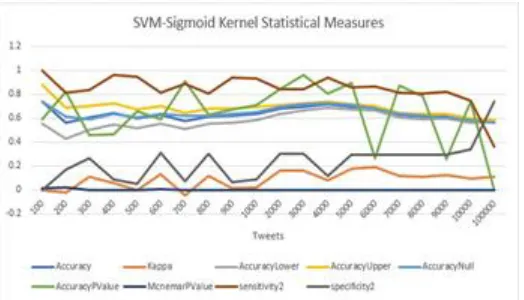
SVM – Sigmoid Kernel and its Performance Metrics: From Fig. 11, this shows the sigmoid kernel does not suit well for analyzing the sentiment under any parameter value and the random movement of all the parameters throughout the tweet count. In other words, SVM under Sigmoid Kernel yield poor results.
Fig. 11 SVM - Sigmoid Kernel Performance Metrics
Fig. 12 Comparison of Accuracy among NB and SVM (all kernels)
Sensitivity Comparison between NB and SVM: As far as sensitivity is concerned, from Fig 13, Linear Kernel based SVM is found better as it remains more or less constant. Next to linear, Radial Kernel SVM will yield almost a good sensitivity value. But Naïve Bayes is not suitable when sensitivity is taken into account of performance metrics.
Fig. 13 Comparison of Sensitivity among NB and SVM (all kernels)
Specificity Comparison between NB and SVM: From Fig. 14, Specificity value of NB is more preferable (remains almost high). On the other hand, SVM with Radial kernel tries to compete with NB specificity, but it fails when number of tweets are less. Specificity calculated using Polynomial kernel is often found missing when different count values are considered.
Fig. 14 Comparison of Specificity among NB and SVM (all kernels)
5 INFERENCES
In general, SVM gives 75% accuracy, whereas NB provides 65% only. In this paper, it is observed that the accuracy value of NB is about 68% (average value) with some fluctuations. While consider SVM, the accuracy value remains almost constant as it provides accurate value nearby to 70% under Radial Kernel. From the above experimentation, Sensitivity value is maximum for SVM based analysis. And hence if one wishes to have good Sensitivity value, they must consider Linear based SVM. Above all, these results are furnished by means of various line charts. In deployment phase, training is done once again in order to check how well the MLA works. From various line charts, it is inference that one can go with Naïve Bayes in terms of Accuracy and Specificity oriented Performance Metrics. Acquiring real time tweets, pre-processing it and feature extraction from the pre-processed data are carried in deployment. While applying Classification Model under NB, by considering less number of tweets say 3000, the predicted result is negative. On the other hand, by increasing the prediction based training dataset up to 1000000 tweets, it gives all the predicted value as positive. Under SVM, while implementing prediction, it gives predicted value as a combination of positive and negative. In other words, SVM provides bidirectional results, whereas NB provides unidirectional values.
6 CONCLUSIONS
In general, SVM gives 75% accuracy, whereas NB provides 65% only. Here it is observed that the accuracy value of NB is about 68% (average value) with some fluctuations. While consider SVM, the accuracy value remains almost constant as it provides accurate value nearby to 70% under Radial Kernel. From various analysis and visualization, it is concluded that it is better to opt SVM with Radial Kernel for Twitter Sentiment Analysis to avoid fluctuations in the result. The second most analysis has been made under NB and tested the working ability of the classifier. If sensitivity is preferred, the linear kernel suits better.
7 FUTURE
ENHANCEMENTS
The task of sentiment analysis, in the domain of micro-blogging, is still in the developing stage and far from complete; Parallelizing code; Detect sarcasm in tweets Adding some of the words that are not considered in the dataset; so as to enhance the betterment of analyzing the sentiment: Extract from newspapers (TOI); Analyzing images for emotions; Since the paper majorly concentrated only on unilingual concept, sometimes multilingual is also preferable i.e. more than one language should also be encountered in analyzing the sentiment since twitter has many varies users from across: Applying sentiment analysis to Facebook messages.
REFERENCES
[1] A. Akshay, J. Niketan, B. Mahavir and M. Venkatesan, "Twitter Sentiment Analysis of Movie Reviews using Machine Learning Techniques," International Journal of Engineering and Technology (IJET), vol. 7, no. 6, pp. 0975-4024, 2016.
Engineering and Technology (IJET), vol. 6, no. 4, pp. 2319-1058, 2016.
[3] A. Vishal, Kharde and S. Sonawane, "Sentiment Analysis of Twitter Data: A Survey of Techniques," Internatinal Journal of Computer Applications, vol. 139, no. 11, pp. 0975-8887, 2016. [4] A. Sonali and P. Asmita, "Twitter Sentiment Analysis and
Visualization," Technical Paper, pp. 2-18, 2016.
[5] M. Walaa, H. Ahmed and K. Hoda, "Sentiment Analysis Algorithms and Applications: A Survey," Ain Shams Engineering Journal, vol. 5, pp. 1093-1113, 2014.
[6] S. Shubham, J. Harshal, P. Pranali, M. Aniket and M. Aniket, "Twitter Data Analysis using R," International Journal of Science Engineering and Technology Research (IJSETR), vol. 6, no. 4, pp. 2278-7798, 2017.
[7] M. Nethu, "Sentiment Analysis in Twitter using Machine Learning Techniques," IEEE, vol. 4, 2013.
[8] G. Alec, B. Richa and H. Lei, "Twitter Sentiment Classification using Distant Supervision," 2009.