* Corresponding author at: Department of Biomedical Engineering, Khalifa University of Science and Technology, and Healthcare Engineering Innovation Center, Abu Dhabi, UAE. cell phone number: , fax number: , [email protected]
Linear and Nonlinear Dynamic Methods towards
1
Investigating Proprioception Impairment in Non-specific
2
Low Back Pain Patients
3
4
Seyed Mohammadreza Shokouhyan
a, Mehrdad Davoudi
a,
5
Maryam Hoviat Talab
a, Mohsen Abedi
b, Soha Bervis
c, Mohamad
6
Parnianpour
a, Simon Brumagne
d, Kinda Khalaf
e *7
8
a
Department of Mechanical Engineering, Sharif University of Technology, Tehran, Iran
9
b
Physiotherapy Research Center, School of Rehabilitation, Shahid Beheshti University of Medical Science, Tehran, Iran
10
c
Physical Therapy Department, School of Rehabilitation sciences, Shiraz University of Medical Science, Shiraz, Iran
11
d
Department of Rehabilitation Sciences, KU Leuven, Leuven, Belgium
12
e
Department of Biomedical Engineering, Khalifa University of Science and Technology, and Healthcare Engineering
13
Innovation Center, Abu Dhabi, UAE
14
15
Abstract
16
Central nervous system (CNS) uses vision, vestibular, and somatosensory information to
17
maintain body stability. Research has shown that there is more lumbar proprioception error
18
among low back pain (LBP) individuals as compared to healthy people. In this study, two
19
groups of 20 healthy people and 20 non-specific low back pain participants (LBP) took part
20
in this investigation. This investigation focused on somatosensory sensors and in order to
21
alter proprioception, a vibrator (frequency of 70Hz, amplitude of 0.5 mm) was placed on the
22
soleus muscle area of each leg and two vibrators were placed bilaterally across the lower
23
back muscles. Individuals, whose vision was occluded, were placed on two surfaces (foam
24
and rigid) on force plate, and trunk angles were recorded simultaneously. Tests were
25
performed in 8 separate trials; the independent variables were vibration (4 levels) and surface
26
(2 levels) for within subjects and 2 groups (healthy and LBP) for between subjects (4×2×2).
27
MANOVA and multi-factor ANOVA tests were done. Linear parameters for center of
28
pressure (COP) (deviation of amplitude, deviation of velocity, phase plane portrait (PPP), and
29
overall mean velocity) and nonlinear parameters for COP and trunk angle ((recurrence
30
quantification analysis) RQA and Lyapunov exponents) were chosen as dependent variables.
31
Results indicated that NSLBP individuals relied more on ankle proprioception for postural
32
stability. Similarly, RQA parameters for the COP on both sides and for the trunk sagittal
33
angle indicated more repeated patterns of movement among the LBP cohort. Analysis of
34
short and long Lyapunov exponents showed that people with LBP caused no use of all joints
35
in their bodies (non-flexible), are less stable than healthy subjects.
36
37
Keywords:
Posture control, low back pain, COP, proprioception, Recurrence Quantification
38
Analysis, Vibrator
39
40
1.
Introduction
41
60 to 80 percent of the world's population have experienced at least one incidence of low back pain
42
(Waddell, 1987; Burton et al., 1995; Méndez and Gómez-Conesa, 2001;
(LBP) in their lifetime
43
Truchon, 2001
)
, with 15% reporting pain in the acute range(Liebenson, 1996)
. Overall, the44
monthly prevalence of LBP is estimated around 23.2%
documented (Hoy et al., 2012). Although
LBP is very common among people between the ages of 35-55(Sarker et al., 2017), it impacts
46
individuals of all ages. Indeed, reports indicate that low back pain represents a prevalent limiting
47
physical factor for adults under 45 years of age, and is considered as the most common cause of
job-48
related disability and a key contributor to missed work days. Health economists estimate that the
49
caring cost for 15% of people with low back pain is equivalent to taking care of 85% of the remaining
50
(Hashemi et al., 1997; Hashemi et al., 1998; Filiz et al., 2005)
population . The cost of treating
51
patients with low back pain has major economic implications. In the U.S. alone, the direct and indirect
52
(Dagenais et al., 2008)
costs associated with LBP range from $84 billion to $624 billion annually .
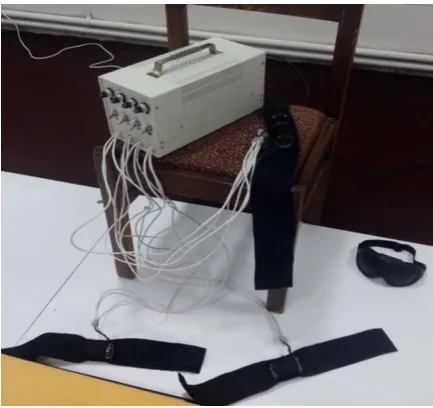
53
In 2006, American insurance claims associated with low back pain were estimated at $100-200
54
(Katz, 2006; Rubin,
billion, 66% of which was due to loss of revenue and reduced productivity
55
2007; Dagenais et al., 2008)
. Importantly, prevalence of LBP has increased by more than 50%56
since 1990, and is projected to continue to increase specially in low and middle income countries
57
(Clark and
(LMICs) where resources are limited and the lifestyle is rapidly becoming more sedentary
58
Horton, 2018)
.59
60
Although postural control for LBP patients is an active area of research, many questions remain
61
unanswered, particularly in terms of changes in sensory input and proprioception. In terms of the
62
physiological processes associated with postural control, it is assumed that once the human neuronal
63
control system senses a deviation associated with the trunk reference location, it sends commands for
64
producing corrective ankle torque to counteract such deviations. This process, however, is highly
65
dependent on the integrity of the three sensory systems: the vision, vestibular, and somatosensory
66
systems. It is likely that the disruption of any one of these systems would negatively impact the final
67
output of the postural system.
68
The proprioception sensory system or central processing of proprioception information may be
69
impaired in individuals with chronic low back pain (della Volpe et al., 2006). It should be noted,
70
however, that the compromised delivery of proprioceptive information does not necessarily disturb
71
the postural function of a person with LBP as he/she may still have sufficient motor control to
72
overcome the deficit. Nonetheless, a disturbed sense of proprioception in people with LBP often
73
impacts their ability to control postural response, particularly when the complexity of postural
74
conditions increases (e.g. walking on unstable or uneven surfaces, standing on one leg, rapid
75
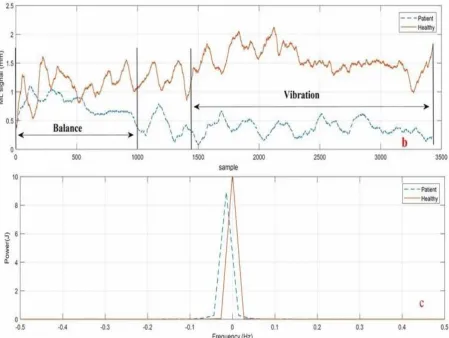
movements of the upper limb (bending), whole body vibration (X), etc.), As such, postural
76
fluctuations and consequent postural control adaptation strategies are likely to significantly increase in
77
LBP patients (della Volpe et al., 2006).
78
Brumagne et al. (Brumagne et al., 2008) indicated that individuals without LBP are more reliant on
79
ankle proprioception while standing on an unstable surface as compared to standing on a stable
80
surface. In contrast, nonspecific low back pain (NSLBP) patients exhibit similar levels of reliance on
81
ankle proprioception regardless of stability conditions. Thus, the ability to discriminately employ
82
ankle proprioception strategy is decreased in NSLBP individuals. Similarly, Claeys et al. (Claeys et
83
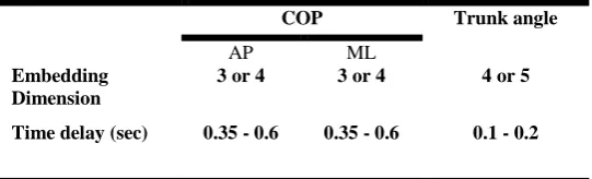
al., 2011) reported decreased variables in postural control strategies among LBP patients during
84
standing and sitting conditions. They found that young people without LBP are able to choose an
85
optimal strategy for postural control based on postural conditions, while conversely, young adults
86
with NSLBP shows reduced variability in self-selected proprioception control strategies. Claeys et al.
87
(Claeys et al., 2012) also evaluated the variability in proprioception during sitting and rising
88
movements, demonstrating that people with low back pain used less lumbar proprioception to control
89
posture in comparison to their healthy counterparts. Claeys et al (Claeys et al., 2015) further examined
90
the potential impact of strategy change for LBP risk, with findings indicating that a higher reliance on
91
ankle-steered proprioception elevated the risk for mild NSLBP. In contrast, fluctuations in postural
92
angle, psychological variables, and physical activity levels did not increase the risk for LBP among
93
the study’s cohort. This study expands previous research by describing a methodology using various
94
advanced linear and nonlinear dynamic analysis tools (RQA and Lyapunov exponents) to quantify and
95
compare proprioception control parameters (body sway and stability) between non-specific low back
96
pain patients and healthy controls towards effective personalized LBP interventional therapy and
97
treatment.
98
2.
Materials and methods
100
2.1.
Subjects specifications
101
40 males participated in this study. The subjects were equally divided into two groups: an NSLBP
102
group and a healthy control group. The number of individuals in each group was estimated using the
103
literature (COP displacement) (Claeys et al., 2011), as well as a G-Power statistical software
104
(Gpower, 2019). The inclusion criteria for the NSLBP patients included being free of vestibular
105
disorders, radiculopathy, neurological, or respiratory disease, in addition to any surgical procedures
106
involving the spine, neck, chest, or lumbar. After all 40 participants completed the required informed
107
consent form approved by the University Internal Ethics Board (approved by IRB of Shahid Beheshti
108
University of Medical Sciences, Tehran, IR, No: IR.SBMU.RETECH.REC.1396.1392), demographic
109
data was recorded including age, height, weight, and BMI index (Table 1). Prior to experimental
110
testing, each individual completed two questionnaires designed to assess LBP by ODI (Oswestry
111
Disability Index) (Fairbank and Pynsent, 2000), and to rate back pain on a numerical scale by NPRS
112
(quantization of pain), respectively (Joos et al., 1991). Individuals were then assigned to the “healthy”
113
group if they reported ODI>6 or NPRS>0. However, all men in the healthy cohort reported zero for
114
both NPRS and ODI questionnaires in this study. If any participant reported any pain at the time of
115
the test, it was postponed to a later date.
116
117
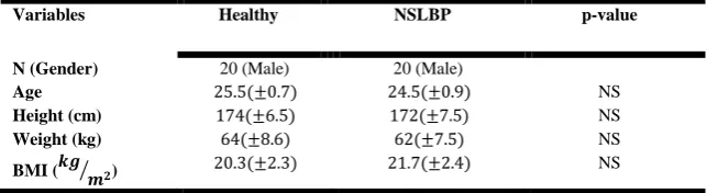
Table 1 :Demographic Data of Healthy and Low Back Patients Participants
118
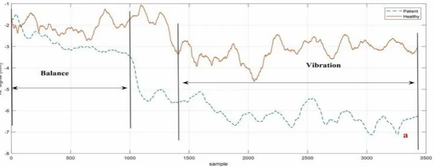
Variables Healthy NSLBP p-value
N (Gender) 20 (Male) 20 (Male)
Age NS
Height (cm) NS
Weight (kg) NS
BMI ( ⁄ ) NS
119
2.2.
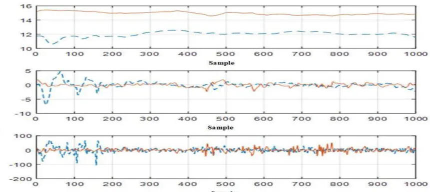
Muscle proprioception
120
There are several ways to alter proprioception input, the most common of which is to externally
121
vibrate the muscles (Goodwin et al., 1972; Roll and Vedel, 1982). In order to alter proprioception of
122
the soleus and lumbar muscles, we developed an in-house vibrator apparatus equipped with four
123
brushless DC motors to produce muscle vibration (Figure 1). The device was placed at the
124
longissimus and multifidus muscles spanning the lumbar vertebrae L3 to L5, as well as in the triceps
125
surae located at the calf of the lower legs. Previous research suggests that optimal proprioception
126
alteration occurs at a frequency of 70 Hz (Goodwin et al., 1972; Roll and Vedel, 1982; Cordo and
127
Gurfinkel, 2004), while another reports a frequency of 60 Hz and an amplitude of 0.5 mm as ideal for
128
altering one’s sense of proprioception (Claeys et al., 2011). The vibration frequency of our device was
129
set to 70 Hz, with amplitude of about 0.5 mm to produce optimal altered proprioceptive data. When
130
the vibrators were applied to the soleus muscles, dorsiflexion was externally induced. In response, the
131
central nervous system (CNS) used the proprioceptive data to move the body rearward to maintain
132
balance. Conversely, when the vibrations were applied to the lumbar area, an extension was externally
133
135
136
Figure 1: in-house vibrator apparatus for producing of muscle vibration
137
2.3.
Procedure
138
A force plate (Bertec USA) was used to record the body's center-of-pressure (COP) fluctuations
139
and to obtain the trunk angles through inverse dynamics. A Vicon optical motion capture system with
140
markers synced to the force plate was used in conjunction. The markers were positioned at the C7,
141
T12, lower sternum (xiphoid process), clavicle (Incisura jugularis), right scapula, right and left sides
142
of the PSIS (posterior superior iliac spine) and ASIS (anterior superior iliac spine) based on literature.
143
The coordinate system was defined such that the axis perpendicular to the individual’s coronal plane
144
was defined as the X-axis (anterior-psoterior (AP)), the axis perpendicular to the sagittal plane was set
145
as the Y-axis (medial-lateral (ML)), and the Z-axis (proximal distal (PD)) was perpendicular to the
146
transverse plane. The selected sampling frequency on both devices was 100 Hz. The motor straps
147
were attached to the end of triceps surae muscle (muscle spindle) on each foot, and on the multifidus
148
muscles bilaterally. Each participant, with occluded vision (using am eye mask), performed 8 separate
149
trials as follows: 1) standing on a motionless rigid surface (without any vibrator-induced movement);
150
2) standing on a rigid surface with the activation of the triceps vibrators; 3) standing on a rigid surface
151
with the activation of the multifidus vibrators; 4) standing on a rigid surface with the activation of
152
both the triceps and multifidus vibrators; 5) standing on a motionless foam surface; 6) standing on a
153
foam surface with the activation of the triceps vibrators; 7) standing on a foam surface with the
154
activation of the multifidus vibrators; and 8) standing on a foam surface with the activation of both the
155
triceps and multifidus vibrators. For each trial, COP data was recorded in both the anterior posterior
156
(AP) and medial lateral (ML) positions; trunk angles were also recorded in the three anatomical
157
planes. Each trial lasted 30 seconds: (1) 10 seconds with the individual standing on the force place in
158
the absence of any vibration (the balance phase); and (2) 20 seconds when the motors were turned on
159
at a frequency of 70 Hz (the vibration phase). The experimental set-up in this study is shown in
160
Figure 2 (written informed consent was obtained from the individuals for the publication of any
161
potentially identifiable images or data included in this article).
162
Figure 2: Experimental set-up
164
2.4.
Filtering and time series separation
165
In order to filter COP and trunk angle data, the exact cutoff frequency was determined acoustically
166
via spectral analysis. The amount of signal energy was determined in terms of the frequency. 99% of
167
signal strength for all COP and trunk sagittal angles was at a frequency of less than 5 Hz; thus, the
168
cutoff frequency of 5 Hz was used for data filtering (Figure 3c). The data was then filtered by
169
selecting a second-order Butterworth non-linear filter, according to literature (Ghomashchi et al.,
170
2011).
171
2.5.
Linear analysis of COP time series
172
In order to analyze center-of-pressure data, the standard deviation of displacement, standard
173
deviation of velocity, the mean total velocity, and the phase plane portrait for both anterior-posterior
174
(AP) and medial-lateral (ML) directions were obtained according to Eq. 5-Eq. 12 Table A
175
(Appendix), in which 𝑥 is the average of balance time series, 𝑥𝑖 corresponds to each point of
176
vibration time series, and indicates the length of the time series.
177
Although COP sway toward balance condition can be explained by linear analysis, it is usually not
178
sufficiently powerful for a detailed kinematic interpretation of physiological signal results. Thus,
179
other nonlinear tools were required, which are explained in the following sections.
180
181
2.6.
Nonlinear analysis of COP time series and trunk angle
182
2.6.1.Phase space reconstruction
183
The phase space for a dynamic system refers to a space in which all possible states are shown.
184
Each possible state for the system represents a point in this space. Although there are several methods
185
for analyzing the nonlinear time series of a phase space for a dynamic system, the Time delay method
186
is most commonly used. The most challenging step of this method is to identify (𝜏) Time Delay and
187
(m) Embedding Dimension. For a time series of scalar variables according to Eq. 1
188
Eq. 1
189
We can construct a vector in the phase space according to Eq. 2 at any time:
190
𝑋 𝑡
𝑖= 𝑥 𝑡
𝑖, 𝑥 𝑡
𝑖+ 𝜏 , 𝑥 𝑡
𝑖+ 𝜏 , … , 𝑥 𝑡
𝑖+ 𝑚 − 𝜏
Eq. 2191
Average Mutual Information (AMI) and False Nearest Neighbors (FNN) represent two standard
192
methods for determining the time-delay parameter and the embedding dimension parameter,
193
respectively (Horak, 2003). MATLAB software was used to reconstruct the phase space. For each
194
individual, the phase space was reconstructed separately for each of the three signals: APCOP,
195
MLCOP, and trunk angle. In most cases, the space embedding dimension for both the COP and trunk
196
angle was 3. The time delay was assumed to be the first minimal relative for each person.
197
Subsequently, the obtained phase space was verified using Chaos Data Analyzer software (Sprott,
198
1998), which confirmed the validity of the embedding dimension value. Time delay and embedding
199
dimension values for COP and trunk data were assessed for each person individually and are
200
summarized in Table 2.
201
202
Table 2: Embedding Dimension and Time delay values used as Input parameters for phase space
203
reconstruction of COP and Trunk angle
204
Trunk angle COP
ML AP
4 or 5 3 or 4
3 or 4 Embedding
Dimension
0.1 - 0.2 0.35 - 0.6
0.35 - 0.6 Time delay (sec)
205
206
2.6.2.RQA method
207
Another prominent method for nonlinear time series analysis is Recurrence Quantification Analysis
208
(RQA). Using this approach, the dynamic properties of a system’s path in a phase space can be
209
represented in a two dimensional space. Riley et al. (Riley et al., 1999) expressed numerical criteria
210
based on diagonal lines in n recurrence plot (RP), which can be used to analyze the amount of
211
recurrence or complexity of the dynamics of an observed time series. In this study, RQA quantitative
212
measurements were calculated using the RQA software (Webber Jr, 2009), developed by Webber et
213
al. (Webber Jr and Zbilut, 2005). The Euclidean norm was used for calculating these criteria and the
214
neighborhood radius was identified (Riley et al., 1999), which was considered 2.5% of the mean
215
distance.
216
2.6.3. Short and Long Terms of Lyapunov
217
Next, the phase space for both the COP and trunk angle time series were reconstructed. 𝑋𝑗 can be
218
determined by exploring through all points such that its distance from the reference 𝑋𝑗 is minimized,
219
according to Eq. 3:
220
𝑑𝑖 = min
𝑋𝑗
𝑋𝑗− 𝑋𝑗 Eq. 3
Where … is a Euclidean norm.
221
A Lyapunov function was used for both the COP (both directions) and trunk angle using Eq. 4:
222
Eq. 4
𝑦 𝑖 =
Δt
ln 𝑑
𝑗𝑖
=
𝜆
𝑖 + 𝑐
Where … expresses the mean of the neighboring data points for all values of j. This function was
223
divided by the sampling time intervals (Rosenstein et al., 1993). The short term time (𝜆𝑆) scale was
224
obtained by the initial slope of the curve for the first few sampling intervals. Similarly, the long-term
225
values for the two exponents represent the divergence of the two neighboring paths of phase space
227
(unstable), while negative values represent the convergence of the two neighboring paths— their
228
combination expresses the relative stability of the system. Large and positive exponents are indicators
229
of the system’s dynamic instability; conversely, the larger and negative the exponents, the greater the
230
stability of the system. For this investigation, the slope of the Lyapunov function in the range of 1 to
231
30 samples determined the short-term Lyapunov, while the slope of the Lyapunov function in the
232
range of 250-500 samples determined the long-term Lyapunov exponent for both the COP and
trunk-233
angle time series.
234
2.7.
Statistical Analysis
235
The results from the linear and nonlinear methods to obtain COP and trunk data were compared using
236
SPSS (SPSSsoftware, 2019),where analysis of variance (ANOVA) and multiple analysis of variance
237
(MANOVA) were employed to check for significant differences. In this study, the independent
238
variables consisted of the group category (healthy or NSLBP), the vibration covered muscular area
239
(triceps, multifidus, none and both), and the foot placement condition (rigid or foam) . The
240
results were considered significant at a level of 𝑃 < . Subsequently, all dependent variables were
241
subjected to multi-factor ANOVA, followed by Bonferroni adjustment/correction of the independent
242
variables(Field, 2013)
.
243
3.
Results
244
As shown in Table 3, the results from the ODI and NPRS questionnaires demonstrate significant
245
differences between the healthy participants and the LBP group.
246
247
248
Table 3: Oswestry Disabity Inventory Questionnaire and Pain Scale results from participants
249
Significant difference Patient
(SD) Healthy
(SD) Questioners
Yes 12.3(3.6)
0 ODI-2 (0-100)
Yes 2.5(1.2)
0 NPRS (0-10)
250
The recorded data associated with the force-plate testing was divided into two 10-second segments
251
(balance part) and one 20-second segment (vibration part). Figure 2 a and2b show the results for the
252
second trial in both directions (AP and ML), while the cutoff frequency (5 Hz) for the sample data is
253
shown in Figure 3c with the person standing on the stationary rigid surface with active triceps
254
vibrators.
255
Figure 3: Divided signal and signal power of COP for a healthy subject and a LBP subject during Trial
257
#2. a) AP direction; b) ML direction; c) signal power
258
259
The trunk kinematics (angular velocity and the angular acceleration) were obtained using
260
sequential numerical derivatives of the trunk angular position. Since the noise effects increase may
261
impact RQA analysis, the derivate was filtered once again. On the other hand, subsequent RQA
262
analyses of angular velocity and angular acceleration data showed unexpected results (positive trend
263
(+1.2)), which we attribute to the noise effect. Therefore, while no analysis was conducted on the
264
angular velocity and acceleration of the trunk, the effect of noise on angular velocity remains
265
uncertain and cannot be factored out from the data analysis. The angular position, velocity and
266
acceleration for the trial #2 are depicted in Figure 4 for both healthy and the LBP participants.
267
Figure 4: Angle, angular velocity, and angular acceleration of trunk in sagittal view for a healthy
269
participant and a LBP participant in Trial #2(ankle vibration on rigid surface).
270
271
All linear parameters are listed in Table A2and Table A3 of the Appendix. Note that the values for
272
the linear parameter data were higher in the LBP individuals as compared with the healthy control in
273
both the AP and ML directions for the rigid and foam conditions. This finding indicates that to
274
maintain balance, the LBP group altered their COP more than their healthy counterparts, which made
275
them more reliant on the ankle proprioception strategy, thereby leading to increased COP variation.
276
These changes were evident when the ankle vibrators were activated on the foam surface
277
(𝝈𝒙=Healthy 18.82< Patient 28.91 and 𝝈𝝊𝒙=Healthy 22.11 < Patient 29.21). Table 4 shows the
278
results of the statistical analyses with linear parameters (units in millimeters).
279
280
Table 4: Results of Three way Analysis of Variance (ANOVA) tests for the effects of Surface, Vibration
281
and Group on the linear parameters of COP
282
r
TotalV
y r
x r
y v
x v
y
x
Independent Variable P F P F P F P F P F P F P F P F Main Effect P<0.05 163.57 P<0.05 277.97 P<0.05 521.18 P<0.05 246.19 P<0.05 162.43 P<0.05 199.67 P<0.05 81.75 P<0.05 11.06 Surface P<0.05 33.67 P<0.05 24.38 P<0.05 67.76 P<0.05 57 P<0.05 18.9 P<0.05 6.35 P<0.05 14.32 P<0.05 53.43 Vibration P<0.05 118.54 P<0.05 72.53 P<0.05 583.19 P<0.05 157.6 P<0.05 84.57 P<0.05 36.56 P<0.05 259.8 P<0.05 69.02 Group Interaction P=0.28 1.28 P<0.05 5.72 P<0.05 9.4 P=0.14 1.82 P=0.06 2.49 P=0.55 0.73 P<0.05 4.1 P=0.06 2.48Surface× Vibration
P<0.05 4.39 P=0.31 1.035 P<0.05 108.51 P=0.19 1.657 P<0.05 16.32 P<0.05 9.74 P<0.05 47.1 P=0.06 3.38 Surface× Group P<0.05 7.72 P<0.05 3.27 P<0.05 26.74 P<0.05 11.61 P<0.05 5.79 P=0.3 1.21 P<0.05 8.8 P<0.05 12 Vibration× Group P=0.85 0.25 P=0.62 0.58 P<0.05 7.77 P=0.39 0.98 P=0.08 2.21 P=0.98 0.05 P<0.05 3.5 P=0.17 1.66 Surface× Vibration× Group
283
The RQA parameters for both the AP and ML directions of COP are shown in
Table A4 and284
Table A5 (Appendix). Note that the value of Recurrence in the LBP cohort, as compared to the
285
healthy group, indicates the presence of repetitive points and more repetitive sway in motor behavior,
286
especially on foam. This was evident in the trials performed with the active vibrators (0.45 > 0.11).
287
Furthermore, the value of Determinism was greater in the LBP group as compared to the healthy
288
individuals. This was more remarkable when the triceps vibrators were activated, especially on foam
289
(99.52 > 96.44), suggesting the reliance on more repetitive patterns among the LBP group.
290
The Entropy value, which expresses the complexity of determinism, was also calculated. Entropy was
291
higher for the LBP group as compared to the healthy group across most of the trials (4.69 > 3.9). The
292
trend is also shown in Table A4and Table A5 (Appendix), which helps explain the non-stationary
293
behavior of the system. Specifically, the amplitude of this parameter was higher in the LBP group
294
statistical analysis of the RQA parameters is shown in Table A6 (Appendix), where most of these
296
parameters indicate significant differences between the LBP and Healthy cohort (P<0.05). Results for
297
the RQA parameters of the trunk data are provided in Table A7 and Table A8 (Appendix). RQA
298
measures based on diagonal lines including Recurrence, determinism, entropy, and trend for each
299
group of the COP time series were calculated from the recurrence plots, as shown in Figure 5 for both
300
cohorts (Trial #6). The concept of RQA parameters and their relationship with the diagonal lines can
301
be found in (van den Hoorn et al., 2018)
.
The results of the statistical analyses are provided inTable302
A9.
303
304
Figure 5: recurrence plot for a healthy (left) and a LBP (right) individual in Trial #6 (ankle vibration on
305
foam surface
306
Short-term and long-term Lyapunov exponents are shown in Table A10 and Table A11 (Appendix)
307
for the COP and trunk angle data. For all the trials, the phase space path stability of the healthy cohort
308
was higher than that of the LBP cohort (less Lyapunov exponents value). These results are consistent
309
with the results of the velocity deviation parameters for both the AP and ML directions as shown in
310
Table A2 and Table A3 (Appendix). Moreover, a direct relationship was observed between
311
instability and the increase of velocity deviation in both cohorts. It can be seen from the short and
312
long-term Lyapunov exponents that the LBP individuals experienced greater problems with stability
313
in comparison with the healthy group under the same testing conditions. Moreover, when the same
314
tests were conducted on the softer surface (foam), those instability differences became more
315
pronounced (𝝀𝒔=Healthy 2.5 < Patient 3.2 and 𝝈𝝊𝒙=Healthy 22.11 < Patient 29.21). Statistical
316
analysis of Lyapunov Exponents are provided in Table A12 (Appendix), where short-term Lyapunov
317
shows more significant differences between LBP and Healthy cohorts as compared to long-term
318
Lyapunov (P<0.05).
319
4.
Discussion
320
This work presents a quantitative methodology that leverages both linear and nonlinear dynamic tools
321
to delineate and discriminate proprioception control in non-specific low back pain patients as
322
compared to healthy individuals.
323
The linear analysis employed here revealed that the standard deviation of amplitude and velocity of
324
the COP were higher among the LBP group as compared to the healthy controls in both AP and ML
325
directions, suggesting that the LBP patients experienced a greater challenge in using the hip control
326
strategy to maintain stability instead of the ankle strategy. This was most apparent in the trials during
327
which the vibrators were active (Trials 8, 7, 6, 4, 3 and 2) and while standing on the foam surface.
328
whether this change of strategy in the LBP cohort is due to a disorder in lumbar proprioception
330
receptors making them unable to send the proprioception data to the brain correctly, or whether the
331
control scheme of the brain is actually altered by the LBP, causing the brain to use less of these data
332
(della Volpe et al., 2006).
333
The nonlinear dynamic analysis, including the analysis of the COP data in terms of recurrence,
334
determinism and entropy in the both directions showed that the LBP individuals have more repetitive
335
patterns and sway as compared to the healthy group. This renders them less able to adapt to the
336
environmental conditions and use prior repetitive sway behavior to maintain stability, particularly
337
while on the foam surface which requires more flexibility and adaptive control behavior. Trend, or
338
the measure of the non-stationary behavior of a system, was shown to be higher among the LBP group
339
reflecting failure to achieve a balance point. In conjunction with an increase in the standard deviation
340
of COP, this may be interpreted as functional brain changes that occur during proprioceptive
341
processing in LBP patients contributing to their postural control impairments. Thus, the brain may be
342
able to obtain different data and identify the equilibrium point by increasing the change in COP
343
(Ghomashchi et al., 2011).
344
Functional stability analyses (Table A10 and Table A11 (Appendix)) based on short-term and
345
long-term Lyapunov stability components demonstrated a higher short-term exponent in the LBP
346
cohort as compared to the healthy group for the COP and trunk data. This indicates reduced stability
347
in LBP individuals, suggesting that these patients are less likely to use their full body potential to
348
maintain stability and instead rely more on their ankle joints. This adaptive control strategy is
349
probably due to the less flexible lumbar area as compared to healthy people.
350
Statistical analyses indicated that for most of the parameters used in this study (linear parameters,
351
RQA and Lyapunov components), there were significant differences between the LBP cohort and the
352
healthy group. This suggests that the methodology introduced here along with the various quantitative
353
parameters could be incorporated in the diagnosis and treatment/rehabilitation of individuals with
354
proprioception disorders, including LBP patients. Specifically, physiotherapists should consider the
355
increased use of therapeutic exercises that encourage the use of hip strategy for maintaining stability
356
and to prevent LBP recurrence. The less complexity in NSLBP behaviors (Table A4 and Table A5)
357
can be explained by their higher muscle coactivation (Guthart and Salisbury, 2000) and higher
358
reliance on the ankle strategy (Brumagne et al., 2008)that may reduce the stabilizing control in the
359
ML direction.
360
A number of limitations must be acknowledged. First, in the absence of a device such as
361
obtain direct angular velocity and angular acceleration of the
gyroscope and accelerometer to362
trunk, we relied on a derivative method for calculating these two parameters, which could
363
have led to unreliable results in analyzing and interpreting the data. Second, we did not
364
employ a direct questionnaire or experimental trial that could have unequivocally identified those
365
with proprioception disorders, the patients self-identified which may have affected the results. While
366
motor control adaptation in LBP has been extensively studied from a motor output perspective, much
367
less attention has been paid to changes in sensory input, specifically proprioception. Future studies are
368
needed to use the quantitative tools proposed here to further investigate the adaptive strategies and
369
their impact on the chronification of LBP.
370
5.
Conclusion
371
This study developed a methodology that leverages linear and nonlinear dynamic tools to
372
quantitatively study proprioception impairment in a cohort of LBP patients. The linear analyses
373
results indicated an increase of the standard deviation of amplitude and velocity among the LBP
374
participants, reflecting that these patients were mechanically challenged while using a hip control
375
strategy to maintain stability, and hence opted for an ankle control strategy instead. Nonlinear
376
analyses of recurrence, determinism, and entropy from the COP in both directions, coupled with the
377
trunk kinematic data, demonstrated that the LBP participants used more repetitive sway kinematics, as
378
conditions. Higher trend values in the LBP group indicated that they engage in more non-stationary
380
sway behaviors. The short-term Lyapunov component was greater in the LBP group suggesting
381
greater physical instability. From a short term perspective, our work suggests that LBP patients tend
382
not to use their full body potential to maintain stability and instead rely on the ankle control strategy,
383
possibly due to a compromised or less flexible lumbar area and/or fear of further injury. Future studies
384
are needed to investigate the long-term impact of impaired proprioceptive signaling and its role in
385
postural control.
386
Acknowledgment
387
This research was supported by Sharif University of Technology. We are grateful to Mr. Hamzeh
388
Asadi and Ms. Zeynab Najafi, who contributed greatly to the development of the vibrating device. We
389
also extend our thanks and appreciation to Dr. Dehghan for assistance in the data-recording section of
390
this research. All of the laboratory tests in this study were conducted at the Biomechanics Laboratory
391
of the Faculty of Rehabilitation, Shahid Beheshti University.
392
393
Conflict of interest
394
None.(Salavati et al., 2009)