A Parallel System with Priority to Preventive Maintenance over Replacement Subject To Maximum Operation and Repair Times

(1)

IJEDR1403063

International Journal of Engineering Development and Research (www.ijedr.org)

3199

A Parallel System with Priority to Preventive

Maintenance over Replacement Subject To Maximum

Operation and Repair Times

R. Rathee, S.C. Malik

Research Scholar, Professor

Department of Statistics, M.D. University, Rohtak-124001, India

________________________________________________________________________________________________________

Abstract - The present study deals with profit analysis of a parallel system of two identical units by giving priority to preventive maintenance of one unit over replacement of the other. Each unit has two modes- operative and complete failure. A single server is provided immediately to conduct the repair activities whenever needed. The preventive maintenance of the unit is done after a maximum operation time up to which no failure occurs. The failed unit is replaced by new one in case its repair is not possible by the server in a given maximum repair time. The unit performs with full efficiency as new after repair and preventive maintenance. All random variables are statistically independent. The distributions for failure time, replacement time and the rate by which unit undergoes for preventive maintenance are taken as negative exponential while that of preventive maintenance, repair and replacement rates are assumed as arbitrary with different probability density functions. The semi-Markov process and regenerative point technique are adopted to derive the expressions for some measures of system effectiveness in steady state. The variation of mean time to system failure (MTSF), availability and profit function has been observed graphically for arbitrary values of various parameters and costs.

Key Words - Parallel system, preventive maintenance, replacement, priority and profit analysis.

I. INTRODUCTION

The main intension of the manufacturers is to get maximum profit by selling their products with minimum efforts. And, they have managed it up to a considerable level by using proper operational and repair techniques in their systems. The method of parallel redundancy has been considered as one of the effective strategies for improving performance of the systems and thus profit. Several studies have been conducted on parallel systems under a common assumption that system can work for a long time without requiring any maintenance. But, this assumption seems to be unrealistic as continued operation and ageing of operable systems reduce their performance, reliability and safety. In such a situation preventive maintenance can be conducted after a specific operation time in order to slow the deterioration process. Kishan and Kumar (2009) studied a parallel system with preventive maintenance. The system of parallel units can be made more profitable by making replacement of the failed unit in case server fails to get its repair in a fixed time. Malik and Gitanjali (2012) obtained reliability measures of a parallel system with replacement of the unit subject to maximum repair time. Furthermore, the concept of priority in repair disciplines is one of the best ideas to enhance the profit of the system. Malik and Nandal (2010), Malik and Sureria (2012) and Kumar et al. (2012) have developed reliability models for the standby systems using the concept of priority. However, the idea of priority to preventive maintenance over replacement has not been introduced while analyzing system reliability models of two or more units.

Thus, the focus of the present study is to fill up this gap while carrying out profit analysis of a parallel system of two identical units. Each unit has two modes- operative and complete failure. A single server is provided immediately to conduct the repair activities whenever needed. The preventive maintenance of the unit is done after a maximum operation time up to which no failure occurs. The failed unit is replaced by new one in case its repair is not possible by the server in a given maximum repair time. Priority is given to preventive maintenance of one unit over the replacement of the other unit. The unit works as new after repair and preventive maintenance. All random variables are statistically independent. The distributions for failure time, replacement time and the rate by which unit undergoes for preventive maintenance are taken as negative exponential while that of preventive maintenance, repair and replacement rates are assumed as arbitrary with different probability density functions. The semi-Markov process and regenerative point technique are adopted to derive the expressions for some measures of system effectiveness in steady state. The variation of mean time to system failure (MTSF), availability and profit function has been observed graphically for arbitrary values of various parameters and costs.

II. NOTATIONS

E/ : Set of regenerative/ non-regenerative states λ : Constant failure rate

α0 : The rate by which system undergoes for preventive maintenance (called maximum constant rate

of operation time)

(2)

IJEDR1403063

3200

time)

FUr /FWr : The unit is failed and under repair/waiting for repair FURp : The unit is failed and under replacement

UPm : The unit is under preventive maintenance WPm : The unit is waiting for preventive maintenance

FUR/FWR : The unit is failed and under repair / waiting for repair continuously from previous state FURP : The unit is failed and under replacement continuously from previous state

UPM : The unit is under preventive maintenance continuously from previous state WPM : The unit is waiting for preventive maintenance continuously from previous state g(t)/G(t) : pdf/cdf of repair time of the unit

f(t)/F(t) : pdf/cdf of preventive maintenance time of the unit r(t)/R(t) : pdf/cdf of replacement time of the unit

qij (t)/ Qij(t) : pdf / cdf of passage time from regenerative state Si to a regenerative stateSj or to a failed state

Sj without visiting any other regenerative state in (0, t]

qij.kr (t)/Qij.kr(t) : pdf/cdf of direct transition time from regenerative state Si to regenerative state Sj or to a failed

state Sj visiting state Sk, Sr once in (0, t]

Mi(t) : Probability that the system up initially in state Si E is up at time t without visiting to any

regenerative state

Wi(t) : Probability that the server is busy in the state Si up to time „t‟ without making any transition to

any other regenerative state or returning to the same state via one or more non-regenerative states.

i : The mean sojourn time in state which is given by

where denotes the time to system failure.

mij : Contribution to mean sojourn time (i) in state Si when system transits directly to state Sj so that

_i _ij j

m







and mij =

*

'

( )

(0)

ij ij

tdQ t

 

q





&

: Symbol for Laplace-Stieltjes convolution/Laplace convolution */** : Symbol for Laplace Transformation /Laplace Stieltjes Transformation The possible transition states of the system model are shown in fig.1

III. TRANSITION PROBABILITIES AND MEAN SOJOURN TIMES

Simple probabilistic considerations yield the following expressions for the non-zero elements as











0

(

)

(

q

t

dt

Q

p

_ij _ij _ij

(1) 01 0

2 ,

2 p



 





0 02 0

,

2 p



 





*

10

(

0 0

),

p



g

 





₁₃ * ₀ ₀

0 0

(1

(

)),

(

)

p



g

 



 









*

40

(

0

),

p



r

 



₄₈ _41.8 * ₀

0

(1

(

)),

(

)

p



r

 







* 0

6,11 66.11 0

0

(1

(

)),

(

)

p



f

 







*

31 56

(

0

),

p



p



g



₄₉ 0 * ₀

0

(1

(

)),

(

)

p



r

 







*

6,10 61.10 0

0

(1

(

)),

(

)

p



f

 







* 0

14 0 0

0 0

(1

(

)),

(

)

p



g

 



 









* *

11.3 0 0 0

0 0

(

)(1

(

)),

(

)

p



g



g

 



 









* 0

15 0 0

0 0

(1

(

)),

(

)

p



g

 



 









* *

0

16.5 0 0 0

0 0

g (

)(1

(

)),

(

)

p





g

 



 









*

37 31.7 59

1 (

0

),

p



p



p

 

g



_19.5 0 * ₀ * ₀ ₀

0 0

(1

(

))(1

(

)),

(

)

p



g



g

 



 









*

60

(

0

),

p



f

 



_11.37 * ₀ * ₀ ₀

0 0

(1

(

))(1

(

)),

(

)

p



g



g

 



 









p

26



p

71



p

81



p

94



p

10,1



p

11,6



1

(2) It can be easily verified that

01 02 10 13 14 15 40 48 49 60 6,10 6,11

1 p



p



p



p



p



p



p



p



p



p



p



p



10 14 11.3 11.37 16.5 19.5 40 41.8 49 60 6,10 66.11

1

(3)

IJEDR1403063

3201

The mean sojourn times ( ) is in the state Si are

0

m

01

m

02







,



₁



m

₁₀



m

₁₃



m

₁₄



m

₁₅ ,



₂



m

₂₆,



₄



m

₄₀



m

₄₈



m

₄₉,

6

m

60

m

6,10

m

6,11







,



₉



m

₉₄

,



₁'



m

₁₀



m

₁₄



m

_11.3



m

_11.37



m

_16.5



m

_19.5

,

'

4

m

40

m

41.8

m

49

,









₆'



m

₆₀



m

_6,10



m

_66.11 (3)

IV. RELIABILITY AND MEAN TIME TO SYSTEM FAILURE (MTSF)

Let



i(t) be the cdf of first passage time from regenerative state Si to a failed state. Regarding the failed state as absorbing

state, we have the following recursive relations for



i(t):

1 02

0

(t)

Q

01

(t)



Q

(t)





&



0 14 4

1

(

t)

Q

10

(

t)



Q

(t)



(

t

)

Q

13

( )

t

Q

15

(t

)





&



&



0

4

(t)

Q

40

(t)



Q

48

(t)

Q

49

( )

t





&



(4) Taking LST of above relation (4) and solving for (s), we have

** *

1 ( )

(s)

s

R

s







(5)

The reliability of the system model can be obtained by taking Inverse Laplace transform of (5). The mean time to system failure (MTSF) is given by

**

0

1 ( )

lim

s

N

MTSF

s

D









(6) Where

0 01 1 01 14 4

N







p





p p



and

D

 

1 p p

_{01 10}



p p p

_{01 14} ₄₀

(7) V. STEADY STATE AVAILABILITY

Let Ai(t) be the probability that the system is in up-state at instant „t‟ given that the system entered regenerative

state Si at t = 0.The recursive relations for

A t

_i

( )

are given as:

0

( )

0

(t) q

01

( )

1

( )

02

(

)

2

( )

A t



M



t



A t



q

t



A t

0 14 4 11.3

1

( )

1

(

t

) q ( )

10

( )

(

) (q

( )

11.37

( ))

1

( )

16.5

( )

6

(t)

19.5

( )

9

( )

t

A

t



M



t



A t



q

t



A t



t



q

t



A t



q

t



A



q

t



A

2

( )

26

( )

6

( )

A

t



q

t



A

t

0 41.8 1 4

4 4 9 9

4

(

)

( )

0

( )

( ) q

( )

( ) q ( )

( )

A t



M t



q

t



A t



t



A t



t



A

t

0 61.10

6

( )

6

( )

60

(

)

A t

( ) q

(

t

)

A t

1

( ) q

66.11

(

t

)

6

( )

A t



M t



q

t











A t

9

( )

q ( )

4

t

A t

4

( )

A t





(8) Where

0

(2 ) 0

( )

t

M t



e

   , ( 0 0)

1

( )

( ) ,

t

M t



e

    

G t

( 0)

4

( )

R( )

t

M t



e

  

t

, ( 0)

6

( )

F( )

t

M t



e

  

t

₍₉₎ Taking LT of above relations (8) and solving for A0*(s). The steady state availability is given by

* 1

0 0

0 ₁

( )

lim

( )

s

N

A

sA s

D



 



(10) Where

1 0

{ (1

1 01

)

4

(

14 19.5

)}

6

and

N





X







p





p



p

Y





Z

' ' '

1

(

0 2

p )

02

{

1

(1

49

)

4

(p

14

p

19.5

)

9

(p p

14 49

p

19.5

)}Y

6

D









X







p













Z

(11) VI. BUSY PERIOD ANALYSIS FOR SERVER

(a) Due to Repair

Let B_iR( )t be the probability that the server is busy in repair the unit at an instant„t‟ given that the system entered regenerative state Si at t=0.The recursive relations for B tiR( )are as follows:

0 01 1

(

02 2

(4)

IJEDR1403063

3202

14 11.3

1

( )

1

(t) q (

10

)

0

( )

4

( ) (q

( )

11.37

( ))

1

( )

16.5

(

)

6

(t)

19.5

( )

9

(t)

R R R R R R

t

q

t

q

t

q

t

q

t

B

t



W



t



B





B





B





B





B

2

( )

26

( )

6

( )

R R

B

t



q

t



B

t

41.8

4

( )

40

( )

0

( ) q

( )

1

(

) q ( )

49 9

( )

R R R R

t

B

t



q

t



B





B

t



t



B

t

6

( )

60

(

)

0

( ) q

61.10

( )

1

( ) q

66.11

( )

6

(

)

R R R R

t

B

t



q

t



B





B





B

t

9

( )

q ( )

4 4

( )

R R

t

B

t





B

(12) Where

0 0 0 0 0 0

( ) ( ) ( )

1

( )

( ) (

1) ( )

(

0

1) ( )

t t t

W

t



e

    

G t





e

    



G t





e

    



G

t

(13) Taking LT of above relations (12) and solving for _B₀R*_{( )}_s .The time for which server is busy due to repair is given by

₀ ₀* 2

0 ₁

( )

lim

(s)

R R

s

N

B

sB

D



 



(14)

Where *

2 1

(0)(1

49

) Y

N



W



P

and D1 is already mentioned. (15)

(b) Due to Replacement

Let B_iRp( )t be the probability that the server is busy in replacement the unit at an instant „t‟ given that the system entered regenerative state Si at t=0.The recursive relations for B_iRp( )t are as follows:

0 01 1 02 2

B

Rp

( )

t



q (

t

)



B

Rp

( )

t



q

(

t

)



B

Rp

( )

t

14 11.3 11.37 16

1

( )

q

10

(

)

0

( )

4

( ) (q

( )

( ))

1

( )

.5

( )

6

(t)

19.5

( )

9

(

t

)

Rp Rp Rp Rp Rp Rp

t

q

t

q

t

B

t



t



B





B





B



q

t



B



q

t



B

2

( )

26

( )

6

( )

Rp Rp

B

t



q

t



B

t

41.8 49

4

( )

4

( )

40

( )

0

( ) q

( )

1

( ) q ( )

9

(

)

Rp Rp Rp Rp

B

t



W t



q

t



B

t



t



B

t



t



B

t

6

( )

60

( )

0

( ) q

61.10

( )

1

( )

q

66. 11

( )

6

( )

Rp Rp Rp Rp

t

B

t



q

t



B





B





B

t

9

(

)

q ( )

4 4

(

)

Rp Rp

t

B

t





B

(16)

Where

0 0

( ) ( )

4

( )

( ) (

1) ( )

t t

W t



e

  

R t





e

  



R t

(17) Taking LT of above relations (16) and solving for *

0 ( )

Rp

B s .The time for which server is busy due to replacement is given by

₀ ₀ * 3

0 ₁

( )

lim

( )

Rp Rp

s

N

B

s

sB

s

D





(18)

Where *

3 4

(0)(

14 19.5

)

N



W

p



p

Y

(c) Due to Preventive Maintenance Let P_{( )}

i

B t be the probability that the server is busy in preventive maintenance the unit at an instant „t‟ given that the system entered regenerative state Si at t=0.The recursive relations for B_iP( )t are as follows:

0 01 1

(

02 2

B (

P

t

)



q

( )

t



B

P

t

)



q

( )

t



B

P

( )

t

14 11.3 11.37 16.5 19

1

( )

q ( )

10 0

( )

4

( ) (q

( )

( ))

1

( )

6

(t

)

.5

( )

9

(t)

P P P P P P

t

q

t

q

t

q

t

q

t

B

t



t



B





B





B





B





B

2

( )

2

(

)

26

(

)

6

(

)

P P

B

t



W t



q

t



B

t

41.8

4

( )

40

( )

0

( ) q

( )

1

(

) q ( )

49 9

( )

P P P P

t

B

t



q

t



B





B

t



t



B

t

61.10 66.1

6

( )

6

( )

60

(

)

0

( ) q

( )

1

(

) q

1

(

)

6

(

)

P P P P

B

t



W t



q

t



B

t



t



B

t



t



B

t

9

(

)

9

( )

t

q (

94

)

4

(

)

P P

(5)

IJEDR1403063

3203

Where

2

( )

9

( )

W t



W t



F t

and

W t

₆

( )



e

 ( 0) t

F t

( ) (





₀

e

 ( 0)t



1) ( ) (

F t





e

 ( 0)t



1) ( )

F t

(21) Taking LT of above relations (20) and solving for B₀P*( )s .The time for which server is busy due to preventive maintenance is given by

₀ ₀* 4

0 ₁

( )

lim

( )

P P

s

N

B

sB

s

D



 



(22)

Where

* * *

4 2

(0)

02 6

(0) Z

9

(0)(p

14 49 19.5

) Y

N



W

p X



W



W

p



p

VII. EXPECTED NUMBER OF REPAIRS

Let _{R t}_i_{( )}be the expected number of repairs by the server in (0, t] given that the system entered the regenerative state Si at t = 0. The recursive relations for R t_i( )are given as:

0

( )

01

(

)

R t

1

( )

Q

02

( )

2

(

)

R t



Q

t

&



t

&

R

t

0 14 4 11.3 1

11.37 1 16.5 6 1

1 1

5 0

9. 9

(1

( ))

( )

(1

( ))

( )

(1

(t)

( )

)

( )

(t)

R t

Q

t

R t

Q

t

R t

Q

t

R t

Q

t

R

Q

t

R

R t

Q

t







&

2

( )

26

(

)

6

( )

R t



Q

t

&

R

t

0 41.8 4 9

40 9

4

(

)

( )

R t

( )

Q

( )

t

R t

1

( )

Q

( )

t

R t

(

)

R t



Q

t

&



&



&

0 61.10 1 66.11

60 6

6

( )

(

)

R t

( )

Q

( )

t

R t

( )

(

)

( )

R t



Q

t

&



&



Q

t

&

R

t

9

( )

4

( )

4

( )

R t



Q

t

&

R t

(24)

Taking LST of above relations (24) and solving for

R

₀**

( )

s

.The expected no. of repairs per unit time by the server are giving by

** 5

0 0

0 ₁

( )

lim

(s)

s

N

R

sR

D



 



(25)

Where

5

(

10 11.3 16.5

)(1

49

)

N



P



P



P



P

Y

VIII. EXPECTED NUMBER OF REPLACEMENTS

Let

Rp t

_i

( )

be the expected number of replacements by the server in (0, t] given that the system entered the regenerative state Si at t = 0. The recursive relations for

Rp t

_i

( )

are given as:

0 2

0

( )

1

( )

Rp t

1

(

)

Q

02

( )

Rp t



Q

t

&



t

&

Rp

t

0 14 4 11.3 1

11.37 1 16

1 10

.5 6 19.5 9

( )

(1

( ))

( )

(t)

( )

(t

(

)

(

Rp t

Q

t

Rp t

Q

t

Rp t

Q

t

Rp t

Q

t

Rp

Q

t

Rp t

Q

Rp

t





&

2 6

2

( )

6

(

)

( )

Rp t



Q

t

&

Rp

t

0 41.8

4

( )

40

( )

(1

Rp t

( ))

Q

( )

t

(1

1

( ))

49

( )

9

( )

Rp t



Q

t

&



&



Rp t



Q

t

&

R

p

t

6

( )

60

(

)

Rp t

0

( )

Q

61.10

( )

t

Rp t

1

( )

Q

66.11

(

)

6

(

)

Rp t



Q

t

&



&



t

&

R

p

t

9 4

9

( )

4

( )

Rp t



Q

t

&

Rp t

(27)

Taking LST of above relations (27) and solving forRp**₀ ( )s .The expected number of replacements per unit time by the server is giving by

₀ ₀** 6

0 ₁

( )

lim

( )

s

N

Rp

sRp

s

D



 



(28)

Where

6

(1

49

)(

14 11.3 19.5

)

N



Y



p



p



p

and D1 is already mentioned. (29) IX. EXPECTED NUMBER OF PREVENTIVE MAINTENANCES

(6)

IJEDR1403063

3204

0

( )

01

(

)

P t

1

( )

Q

02

( )

2

(

)

P t



Q

t

&



t

&

P

t

0 14 4 11.3 11.37

1 10 1

16.5 6 19.5 9

(

)

( )

(

( )

( ))

( )

P (t)

( )

(t)

P t

Q

t

P t

Q

t

Q

t

P t

Q

t

Q

t

P

P t



Q

t



&

2

( )

Q

26

( )

t

(1

P

6

( ))

t

P t



&



0 41.8 4 9

40 9

4

(

)

( )

P t

( )

Q

( )

t

P t

1

( )

Q

( )

t

P t

(

)

P t



Q

t

&



&



&

0 61.10 1 66.

6

(

)

60

( )

(1

P t

( ))

Q

( )

t

(1

P t

( ))

Q

11

( )

t

(1

6

( )

)

P t



Q

t

&



&



&



P t

9

( )

Q

4

( )

t

(1

P t

4

( )

)

P t



&



(30) Taking LST of above relations (30) and solving for **

0 ( )

P s .The expected number of preventive maintenances per unit time by the

server is giving by

** 7

0 0

0 ₁

( )

lim

( )

s

N

P

sP

s

D



 



(31)

Where

7 02

(

14 49 19.5

)

N



p X



p p



p

Y



Z

Where

49 11.3 11.37 66.11 61.10 16.5 41.8 66.11 14 19.5

(1

){(1

)(1

) p

}

(1

)(

)

X

 

p



p



p



p



p



p



p



p

01

(1

66.11

)

61.10 02

Y



p



p



p

49 01 16.5 11.3 11.37 02 02 41.8 14 19.5

(1

){

(1

)

}

(

)

Z

 

p

p p

 

p



p



p p

p



p

(33) X. PROFIT ANALYSIS

The profit incurred to the system model in steady state can be obtained as

0 0 1 0 2 0 3 0 4 0 5 0 6 0

Rp

R P

P



K A



K B



K B



K B



K R



K Rp



K P

(34) Where

P = Profit of the system model

K0 = Revenue per unit up-time of the system

K1 = Cost per unit time for which server is busy due to repair

K2 = Cost per unit time for which server is busy due to replacement

K3 = Cost per unit time for which server is busy due to preventive maintenance

K4 = Cost per unit time repair

K5 = Cost per unit time replacement

K6 = Cost per unit time preventive maintenance

XI. CONCLUSION

The results for some important reliability measures have been evaluated for the particular case

g t

( )

=



et, r t( ) =__et_,

( )

f t =



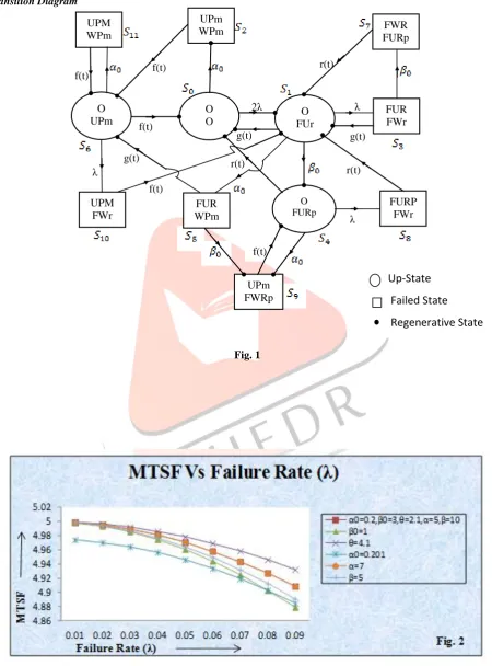
et. Graphs are drawn to show the behavior of MTSF, availability and profit with respect to failure rate (λ) as shown in figures 2, 3 and 4 respectively. It is observed that MTSF, availability and profit go on decreasing with the increase of failure rate (λ) and the rate (α0) by which unit undergoes for preventive maintenance while their values increase with the increase of repair rate (θ) and replacement rate (β). MTSF and availability keep on increasing as the rate (β0) by which unit undergoes for replacement increases while system becomes less profitable. Also, there is no effect of preventive maintenance rate (α) on MTSF whereas system becomes more profitable with the increase of preventive maintenance rate (α). Thus, the study reveals that a parallel system of two identical units in which priority to preventive maintenance is given over replacement can be made more reliable and profitable to use by increasing repair, preventive maintenance and replacement rates.

REFERENCES

[1] R. Kishan and M. Kumar, “Stochastic analysis of a two-unit parallel system with preventive maintenance”, Journal of Reliability and Statistical Studies, vol. 22, pp. 31- 38, 2009.

[2] S.C. Malik and P. Nandal, “Cost-analysis of stochastic models with priority to repair over preventive maintenance subject to maximum operation time”, Learning Manual on Modeling, Optimization and Their Applications, Edited Book, Excel India Publishers, pp165-178, 2010.

[3] S.C. Malik and Kumar Ashish, “Stochastic modeling of a computer system with priority to PM over S/W replacement subject to maximum operation and repair times”, International Journal of Computer Applications, vol.43 (3), pp. 27-34, 2012.

(7)

IJEDR1403063

3205

[5] S.C. Malik and Gitanjali, “Cost-benefit analysis of a parallel system with arrival time of the server and maximum repair

time”, International Journal of Computer Applications, vol.46 (5), pp. 39-44, 2012.

State Transition Diagram

Fig. 1

r(t)

g(t)

r(t)

f(t) r(t) f(t)

g(t)

f(t) f(t)

f(t)

g(t)

λ λ

λ

2λ UPM

WPm

UPm

WPm FWR

FURp

UPm FWRp UPM

FWr

FUR WPm

FURP FWr FUR FWr O

UPm

O FURp O

O

O FUr

Up-State

Failed State

Regenerative State

(8)