A Graphical Survey of the Various Trajectories of Thermal Electrons in Fu & Fu’s Heat-electric Conversion Xinyong Fu & Zitao Fu 2020/7/30 [email protected] [email protected] Key words Maxwell’s demon magnetic demon entropy decrease entropy elimination

(1)

A Graphical Survey of the Various Trajectories of Thermal

Electrons in Fu & Fu’s Heat-electric Conversion

Xinyong Fu & Zitao Fu 2020/7/30

Key words

Maxwell’s demon magnetic demon

entropy decrease entropy elimination

Abstract

This is a graphical survey of the various thermal electron trajectories

and their contribution to the output current in Fu and Fu’s experiment of

heat-electric conversion. The thermal electrons were emitted at room

temperature from two symmetric Ag-O-Cs surfaces in a vacuum tube,

with various exiting angles, speeds, and exiting spots. Due to the

magnetic field, a certain part of the thermal electrons were transferred

from A to B or from B to A, and the survey shows that the former

exceeds the latter a little bit more, resulting in an electric charge

distributio

n,

with A positively charged and B negatively (or vice versa).

A potential difference between A and B emerges, enabling an output

(2)

Introduction

In our experiment of electron tube FX12-51, two identical and parallel

Ag-O-Cs surfaces (work function 0.8eV) ceaselessly emit thermal

electrons at room temperature. The speeds of the thermal electrons, as

discovered by Richardson in his famous retarding potential experiments

in 1907~1909, are governed by Maxwell’s gas molecule speed

distribution law,

dv

v

e

kT

m

n

dv

v

f

k Tv

m

2 2

2

3 2

)

2 (

4 )

(







₍₁₎

Fig.1

Maxwell’s speed distribution law

volume distribution, three-dimension speed

Equation (1) and Fig.1 gives the numbers of gas molecules or thermal

electrons

in unit space

volume

(n = N/V) and in the speed interval from

v to v + dv for an equilibrium state at temperature T.

It is a

volume distribution.

(3)

and the mean kinetic energy of the gas molecules or thermal electrons by

equation (1).

m

kT

v

_p



2 m

kT

v



8 

m

kT

v

2



3 kT

2

3 



₍₂₎

Maxwell’s speed distribution concentrates in the speed range of

0.125v

p

~ 2.75v

p

, here v

p

is

the most probable speed

of the gas

molecules or thermal electrons.

0.125v

p

< v <

2.75v

p

,

⊿

N

/

N = 99.70%

When a static uniform magnetic field is applied to the electron tube in

the direction of the axis of the tube, along axis OZ, as shown in Fig.2 (b),

the electrons will fly clockwise in the XOY plane along circles of

different radii according to the component of their speed in the XOY

plane, u

u

eB

m

R



u



v

_x2



v

_y2

₍₃

₎

(4)

Hence, for the graphical survey of the trajectories of the thermal

electrons in the XOY plane, we need a Maxwell’s speed distribution of

two dimensions.

The Maxwell’s velocity distribution of three dimensions may also take

the following form,

z y x v v v kT m z y x z y

x

e

dv

kT

m

n

dv

v

f

32 2 ( x y z )

2 2 2

)

2 (

)

,

(



  



. (4)

By integration over all the v

z

, equation (4) reduces to two dimensions

y x v v k T m y x y

x

e

dv

kT

m

n

dv

v

f

2 ( x y )

2 2

)

2 (

)

,

(



 



With a cylindrical coordinate system, we may have

udu

e

kT

m

n

du

u

f

k Tu

m



)

2

2 (

)

(

2 2 



udu

e

kT

m

n

du

u

f

k Tu

m 2

2

)

(



 

₍₅₎

It is the number of gas molecules or thermal electrons

in unit volume

and

in the speed interval from u to u+d u. This is also a

volume distribution

,

and speed u is of two dimensions.

Moreover, in the case of our experiment, for all the trajectories, the

thermal electrons are just ejected from the two emitters and will soon

return back to them. The speed distribution of the ejected electrons is

actually not a volume distribution, but a

beam distribution

, or a

wall

emission distribution

,.

(5)

It is a

gas molecule hole-passing or wall colliding speed distribution, or,

a thermal electron wall emission speed distribution. Conventionally, all

these are called the

beam distribution.

Beam speed distribution of two dimensions

(For beam speed distribution of gas molecules or thermal electrons of

three dimensions, see the appendix.)

As shown in Fig 3, at time t, all the gas molecules or thermal electrons

in a cylinder udtdAcos





with a speed from u to u + du and in the

Fig 3 the number of molecules of u ~ u + du and  dpass dA in dt

direction from





to





+ d





will pass through the hole

dA on the

separation in a duration dt, and their number is

(6)

The factor cos





repersents Lambert law.

For

dA

= 1 and

dt

= 1, and integrate over





from



to



we

derive

du

u

e

kT

m

n

u

d

k Tu

m 2 2 2

)

(









(6

)

The general collision ( or emission) number of thermal electrons in unit

time and on unit area is the so called

wall collision number (or wall

emission number)

, which may be derived by integrate (6) over u from 0

to

∞

Briefly

n

u

4

1 



(7

)

The beam distribution, i.e., the ratio of the number of molecules or

thermal electrons of speed interval u ~ u+du in the beam to the number of

the molecules or thermal electrons of all speeds in the same beam, is

(8)

m

kT

n

m

kT

m

n

du

u

e

kT

m

n

k Tu

m



8

4

1 )

2 (

4

1

₂3

2 2 2













u

n

du

u

e

kT

m

n

d

du

u

g

u k T m

4

1 )

(

2 2 2 









du

u

e

kT

m

du

u

g

k Tu

(7)

Fig 4 Beam distribution, two-dimensional speed

The two different distribution functions, equation (1) and (8), one

is the volume distribution of three dimensions and the other is the

beam distribution of two dimensions, are alike exactly!

We may also easily derive the three characteristic speeds and the mean

kinetic energy of the gas molecules or thermal electrons for the beam

distribution of two dimensional speeds,

m

kT

u

_p



2 m

kT

u



8 

m

kT

u

2



3 kT

2

3 



₍₉

₎

Equation (2) and (9) are also alike exactly.

The beam distribution of two dimensions also concentrates in the speed

range of 0.125u

p

~2.75u

p

, here u

p

is

the most probable speed

of u, u

p

= v

p.

Divide the area under the beam distribution graph of Fig 4 into nine

parts, A0, A1, A2, A3, A4, A5 A6, A7, A

∞

, as shown in Fig 5: for A0 ,



u =

0.25u

p

, for each of A1 to A7,



u

= 0.5u

p

, and for A

∞

,



u

=

∞

(

from

(8)

Fig 5 The nine areas under Maxwell’s beam distribution, two dimensional speeds.

Table 1 The nine areas under Maxwell’s distribution graph, ∑Ai=100% (beam distribution, two dimensions)

Range of speed



u

N

A

ui ui ui ui

i ~ 0 ~ 0 ) ~

( 1





1







 

0.0 ~ 0.25

u

p

0.0 ~ 0.125

u

p

0.125 ~ 0.25

u

p

0.25 ~ 0.75

u

p

0.75 ~ 1.25

u

p

1.25 ~ 1.75

u

p

1.75 ~ 2.25

u

p

2.25 ~ 2.75

u

p

2.75 ~ 3.25

u

p

3.25 ~ 3.75

u

p

3.75 u

p

~

∞

A0 =

〔

0.276326 - 0.265004

〕

= 0.011358 = 1.13%

A

01

=

〔

0.140222-138860

〕

= 0.001362 = 0.14 %

A

02

=

〔

0.011358-0.001362

〕

= 0.009996 = 0.99%

A1 = 0.228958 - 0.011358 = 0.217599 = 21.76%

A2 = 0.627286 - 0.228958 = 0.398328 = 39.83%

A3 = 0.894316 - 0.627249 = 0.267067 = 26.71%

A4 = 0.982467 - 0.894316 = 0.088151 = 8.82%

A5 = 0.998287 - 0.982467 = 0.015820 = 1.58%

A6 = 0.999900 - 0.998287 = 0.001613 = 0.16%

A7 = 0.999996 - 0.999901 = 0.00009

5≈

0.01%

(9)

Calculate with the help of error functions the relative ratios of numbers

of gas molecules or thermal electrons in the nine ranges, and the results

are listed in Table 1. The error functions are

d x

x

e

N

d u

u

e

u

N

d u

u

e

kT

m

N

x v u u p u u k T m u u p 2 0 2 2 0 2 2 2 3 0 ~ 0 2 2 2 2 3 2

4 )

1 (

4 )

2 (

4

  







































   



2 2 2 2

2 )

(

)

(

2

1

2

1

4

0 0 2 0 ~ 0 x x x x x x x v

xe

x

erf

xe

d

dx

e

dx

x

e

N



Now, taking equation (8), Fig 5 and table 2 together as a new platform,

we begin our graphical survey of the various trajectories of thermal

electrons in such an experiment. What we deal with hereafter is the wall

emission distribution of thermal electrons (beam distribution), and the

speeds are of two dimensions.

When a magnetic field is applied to the electron tube, thermal

electrons of the nine different ranges of speed u contribute to the

output current very differently. There are two causes.

The first cause, of course, is Maxwell’s speed distribution itself (beam

distribution, two dimensions). The numbers of electrons in the nine

different speed ranges, as shown in Fig.5 and table 2, are explicitly

different, hence their contributions to the output current are explicitly

(10)

The second cause is that the trajectories of the thermal electrons of

different speeds also related to the exiting angles and exiting spots, are

tremendously different. Tremendously different trajectories result in

tremendously different contributions to the output current.

Fig 6 The cross section of an ideal simple and symmetric electron tube, (1 : 1)

For simplicity of discussion, we analyze here the electron migration

between A and B with an ideal simple and symmetric tube as shown in

Fig.6, which is alike to FX12-51, the actual tube in our experiment,

meanwhile the two tubes have some differences from each other, as

shown in Fig.7.

(11)

At 20

o

_{C, the mean speed of the thermal electrons is}

_u



₁₀₆

_km

_/

_s

_,

compare to the mean velocity of common gas molecules (say, the remnant

gas molecules in the same tube), 460 m/s,

they are extremely fast!

The mean free path of thermal electrons in a vacuum of 10

-6

mmHg is

determined by their collisions with the remnant gas molecules, about 50m,

which is much greater than the dimensions of our tube,



mm

×

L

60 mm.

Hence, these collisions may be neglected and the actual free paths of the

thermal electrons in the tube may be regarded to be just determined by

their ejection from the emitters, their collisions with the tube’s glass wall,

and their absorption by the emitters.

Numerous thermal electrons frequently collide with the glass wall.

These collisions are due to the kinetic energy of their quick motion. At t =

20

o

_{C, the average kinetic energy of the thermal electrons and also of the}

remnant molecules is,

(10)

So, the collisions are extremely weak. The glass wall is sufficiently hard

and smooth for such collisions, and may be regarded here as a perfect

elastic solid.

Now, we start the graphic method to survey the numerous various

trajectories of the thermal electrons emitted from A or B in a magnetic

field with different exiting angles, different speeds, and different exiting

(12)

All the electron trajectories in the tube may be classified into four

groups: A-A, B-B,

A-B

,

B-A

．

Here

directly means no collision with the

glass wall.

A-A = A-directly-A + A-glass-A B-B = B-directly-B + B-glass-B

A-B

=

A-directly-B

+

A-glass-B

B-A

=

B-glass-A

The whole graphical survey has about 150 pages, 250 trajectory figures.

The following

representative exiting angles and speeds are selected for

drawing the trajectories:



= 0

o

, -15

o

, 15

o

, -30

o

, 30

o

, -45

o

, 45

o

, -60

o

, 60

o

, -75

o

, 75

o

u = 0.5u

p,

u

p,

1.5u

p,

2u

p,

2.5u

p,

3u

p,

3.5u

p,

4.5u

p.

We divided the survey into two parts, the first part and the second part.

If the readers have enough time, we suggest them read the whole survey,

which is rather long, but very interesting, comprehensive and beneficial.

However, many readers may have not so much time to read the whole

survey. We suggest them to read just the first part, which deals with only

the thermal electrons emitted vertically from A or B (



= 0

o

_{) with}

different speeds. It has only 16 pages, 33 trajectory figures, providing a

(13)

The First Part of the survey( 

= 0

o



In this first part, we survey all the trajectories of electrons that emitted

vertically (



= 0

o

) from all the points of the two Ag-O-Cs surfaces of the

ideal electron tube shown in Fig.7 (left) with the following representative

exiting speeds,

u =

0.125u

p

, 0.25u

p

, 0.5u

p

,

u

p

,

1.5u

p

, 2u

p

, 2.5u

p

,

3u

p

, 4.5u

p

.

According to Lambert cosine law, normal is the direction of the

strongest emission,

j

∝

cos



.

For convenience of drawing and discussion, as we have mentioned

previously, we choose a static uniform magnetic field of a special

magnetic induction intensity,

B

= 1.34

×10

-4

tesla

= 1.34 gausses, to be

applied to the ideal electron tube in the direction parallel to the tube axis.

In such a magnetic field, for t = 20

o

C, the thermal electrons of speed of u

=

u

p

= 94.3km/s rotate with a radius of

R = 4mm (more precisely,

4.002mm). Thus, for the electrons of speed u = 0.5u

p

, the corresponding

radius is R

=2mm. For the electrons of speed u = 2u

p

, R = 8mm. The rest

may de deduced by analogy.

(14)

1. Trajectories of electrons of 

= 0

o

_{and different speeds u}

(1) Fig 1-1



= 0

o

_{u = u}

p

R = 4mm (B =1.34 gauss)

(a) A-directly-A & B-directly-B (b) B-glass-B

(from EM to PO, ON to QF, grey) (from C to F, D to U, etc., green) No electron migration between A and B due to these trajectories.

(c) A-directly-B (d) B-glass-A  (from MO to ON, red) (from J to K, G to H, etc, blue)

(MO=40, EO=70) (from DF to B, DF=35, OF=70) MO/EO = 40/70 = 0.57 DF/OF = 35/70 = 0.50 A-B 57% of the electrons of (0o_{, up)}_{emitted from A migrate to B,}

B-A 50% of the electrons of (0o, up)emitted from B migrate to A.

For all the electrons of (0o, up), migration A-B exceeds B-A, and their difference (equals CD) is the corresponding contribution to the output current

(15)

(2)

Fig 1-2



= 0

o

_{u = 0.5u}

p

R = 2mm (

cos

0

o





(a) A-directly-A & B-directly-B (b) B-glass-B No electron migration between A and B due to these trajectories.



(c) A-directly-B (d) B-glass-A (from M to O, P to Q, O to ON, etc., red) (from J to K, etc., blue) (from MO to ON, MO=20, EO=70) (from DF to B, DF =17.5, OF = 70)

MO/EO=20/70=0.29 DF/OF=17.5/70=0.25

A-B 29% of the electrons of (0o, 0.5up)emitted from A migrate to B. B-A 25% of the electrons of (0o, 0.5up)emitted from B migrate to A.

For all the electrons of (0o, 0.5up), migration A-B exceeds B-A, and their difference is the corresponding contribution to the output current

(16)

(3) Fig 1-3



= 0

o

_{u = 0.25u}

p

R = 1mm



(c) A-directly-B (d) B-glass-A (from MO to ON, red) (from J to K, etc., blue)

(MO=10, EO=70) (DF =8.5, OF = 70) MO/EO=10/70=0.14 DF/OF=8.5/70=0.12

A-B 14% of the electrons of (0o, 0.25up)emitted from A migrate to B. B-A 12% of the electrons of (0o, 0.25up)emitted from B migrate to A.

For all the electrons of (0o_{, 0.25up), A-B exceeds}_{B-A, and their difference is the}

corresponding contribution to the output current.

(17)

(4) Fig 1-4



= 0

o

_{u = 0.125u}

p

R = 0.5mm



(c) A-directly-B (d) B-glass-A (from MO to ON) from J to K, etc.)

(MO=5, EO=70) (DF = 4.5, OF = 70) MO/EO=5/70=0.071 DF/OF=4.5/70=0.064 A-B 7.1% of the electrons of (0o, 0.125up)emitted from A migrate to B. B-A 6.4% of the electrons of (0o, 0.125up)emitted from B migrate to A.

(18)

Now, let us see the trajectories of the faster electrons.

(5) Fig 1-5



= 0

o

_{u = 1.5u}

p

R = 6mm



(c) A-directly-B (d) B-glass-A (from PO to OQ, red) (from J to K, G to H, etc., blue)

(PO=60, EO=70) (DF =50, OF = 70) PO/EO=60/70=0.857 DF/OF=50/70=0.714 A-B 85.7% of the electrons of (0o, 1.5up)emitted from A migrate to B. B-A 71.4% of the electrons of (0o, 1.5up)emitted from B migrate to A.

For all the electrons of (0o, 1.5up),A-B exceeds B-A, and their difference is the corresponding contribution to the output current

(19)

(6) Fig 1-6



= 0

o

_{u = 2 u}

p

R = 8mm

(a) B-glass-B

(from C to E, D to V, CD = 3, green)

No electron migration between A and B due to these trajectories.

 (b) A-directly-B & A-glass-B (c) B-glass-A

(red, violet) (from J to K, G to H, etc., blue) (EP+PO=EO =70, EO=70) (DF =67, OF = 70)

EO/EO=70/70=1.00 DF/OF=67/70=0.96 A-B 100% of the electrons of (0o, 2up)emitted from A migrate to B. B-A 96% of the electrons of (0o, 2 up)emitted from B migrate to A.

For all the electrons of (0o, 2up), A-B exceeds B-A, and their difference is the corresponding contribution to the output current.

(20)

(7) Fig 1-7



= 0

o

_{u = 2.5 u}

p

R = 10mm

(a) A-directly-B (red) (b) A-glass-B (violet) A-B = A-directly-B + A-glass-B EM + MO = 70

(EM +MO)/EO =70/70 = 1.00

A-B 100% of the electrons of (0o_{, 2.5up)}_{emitted from A migrate to B.}

(c) B-glass-A (blue) OF/OF = 1.00

B-A 100% of the electrons of (0o, 2.5up) emitted from B migrate to A.

For all the electrons of (0o, 2.5up), A-B and B-A cancel each other, there is no net contribution to the output current.

(21)

(8)

Fig 1-8



= 0

o

u = 3u

p

R = 12mm

(a) A-B = A-directly-B (red) + A-glass-B (violet) 70/70=1.00

A-B 100% of the electrons of (0o_{, 3up)}_{emitted from A migrate to B.}

(b) B-glass-A (from G to H, J to K, etc. blue)

70/70 = 1.00

B-A 100% of the electrons of (0o, 3up) emitted from B migrate to A.

For all the electrons of (0o, 3up), A-B and B-A cancel each other, there is no net contribution to the output current..

(22)

(9) Fig 1-9



= 0

o

_{u = 3.5u}

p

R = 14mm

(a) A-directly-B (red), A-glass-B (violet) A-B = A-directly-B +A-glass-B (red + violet)

70/70 = 1.00

A-B 100% of the electrons of (0o_{, 3.5up)}_{emitted from A migrate to B.}

(b) B-glass-A

(from G to H, J to K, etc.) (OF = 70, blue) 70/70 = 1.00

B-A 100% of the electrons of (0o, 3.5up)emitted from B migrate to A.

For all the electrons of (0o, 3.5up), migrations A-B and B-A cancel each other, there is no net contribution to the output current.

(23)

(10) Fig 1-10



= 0

o

_{u = 4.5 u}

p

R = 18mm

_(a)_A-glass-B

EO/EO = 70/70 = 1.00 (violet)

A-B 100% of the electrons of (0o, 4.5up) emitted from A migrate to B.

(b) B-glass-A OF/OF = 70/70 =1.00 (blue)

A-B 100% of the electrons of (0o_{, 4.5up) emitted from B migrate to A.}

For all the electrons of (0o, 4.5up), migrations A-B and B-A cancel each other, there is no net contribution to the output current.

(24)

(11) Fig 1-11



= 0

o

_u

_{>> 4.5 u}

p

R >> 18mm

(i.e.,



= 0

o \

_{u =}

_∞

R

= ∞

)

(a)

A-glass-B & B-glass-A

(Red and blue)

(from M to N, G to H; from P to Q, J to K; etc.)

D

0o

(

u

∞

) =

｛

(A-B) – (B-A)

｝

0o∞

= 1.00 - 1.00 = 0.

For thermal electrons of extremely high speed, their trajectories are

approximately straight lines although a magnetic field is applied.

Statistically, the electrons are now in symmetric pairs (mirror reflect

symmetry, left-right symmetry), one electron exits from A and the other

from B, with the same speeds, symmetric exiting angles and exiting spots,

and they have symmetric trajectories. Their contributions to the output

(25)

Every 100 + 100 electrons (1.00 = 100% from A, 1.00 = 100% from B)

of exiting angle



= 0

o

and of different speeds contribute to the electron

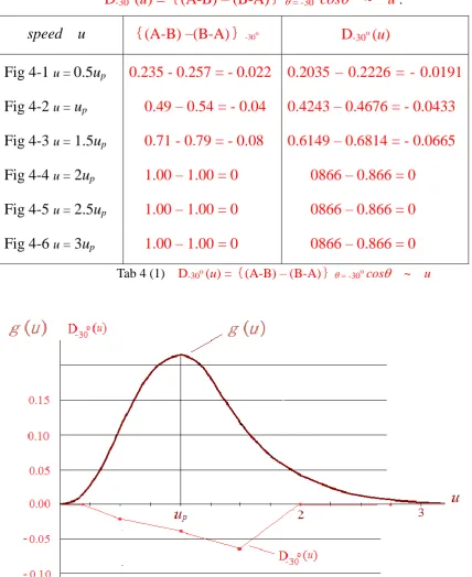
migration between A and B differently, as list in Tab 1 (1) (

cos

0

o





D

0o

(

u

) =

｛

(A-B)–(B-A)

｝

0o

cos



(

u

)

speed u

﹛

(A-B) - (B-A)

﹜

0o

D

0o

(

u

)

=

｛(A-B)–(B-A)｝0o

cos



(

u)

Fig 1-4

u = 0.125u

p

Fig 1-3

u = 0.25u

p

Fig 1-2

u = 0.5u

p

Fig 1-1

u = u

p

Fig 1-5

u = 1.5u

p

Fig 1-6

u = 2u

p

Fig 1-7

u = 2.5u

p

Fig 1-8

u = 3u

p

Fig 1-9

u = 3.5u

p

Fig 1-10

u = 4.5u

p

Fig 1-11

u =

∞

0.07 - 0.06 = 0.01

0.14 - 0.12 = 0.02

0.29 - 0.25 = 0.04

0.57 - 0.50 = 0.07

0.857 - 0.714 = 0.14

1.00 - 0.96 = 0.04

1.00 - 1.00 = 0

0.07 - 0.06 = 0.01

0.14 - 0.12 = 0.02

0.29 - 0.25 = 0.04

0.57 - 0.50 = 0.07

0.857 - 0.714 = 0.14

1.00 - 0.96 = 0.04

1.00 - 1.00 = 0

Tab. 1 (1) the contributions of the electrons of



= 0

o

and

of different speed,

D

0o

(

u

) =

｛

(A-B)–(B-A)

｝

0o

cos



(

u

)



.

(26)

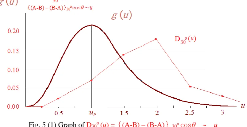
Fig 1 (1) is the corresponding graph,

D

0o

(

u

)

=｛(A-B)–(B-A)｝0o

~

u

\

(27)

Take Maxwell’s speed distribution g

(

u

)

into account to derive the actual

contributions of the thermal electrons of



= 0

o

_{and of different speed}

ranges

⊿

u

, i.e.,

N N

i i u

u~ )

( 1



×

D

0o

(

u

)

⊿

u

~

u

,

Speed range

⊿

_u

_(u

_i

_{~ u}

_{i + 1}

₎

N

i i u

u~ ) ( 1



_D

₀o

₍

_u

₎

｛(A-B)–(B-A)｝0ocos(u)

N

i i u

u~ ) ( 1



×

D

0o

(

u

)

⊿

u

0.00~0.125u

p

0.125~0.25u

p

0.25~0.75u

p

0.75~1.25u

p

1.25~1.75u

p

1.75 ~ 2.25u

p

2.25 ~ 2.75u

p

2.75 ~ 3.25u

p

3.25 ~ 3.75u

p

3.75u

p

~ ∞

A01

= 0.15%

A02

= 4.00%

A1

= 18.74%

A2

= 39.83%

A3

= 26.71%

A4

= 8.82%

A5

= 1.58%

A6

= 0.16%

A7

=

.0096%

A8

=

.0003%

0.07 - 0.06 = 0.01

0.14 - 0.12 = 0.02

0.29 - 0.25 = 0.04

0.57 - 0.50 = 0.07

0.857 - .714 = 0.14

1.00 - 0.96 = 0.04

1.00 - 1.00 = 0

0.15×

0.01 ×

0.125 (triangle



= 0.0001875

≈ 0.0002





× (0.02+0.01) × 0.5 ×

0.125 =

0.0075 (trapezoid



5.4346 – 4.685 = 0.7496

22.7031 -19,915 = 2.7881

22.8905–19.0709= 3.8196

8.82 – 8.4672 = 0.3528

1.58 – 1.58 = 0

0.16 - 0.16 = 0

0.0096 -0.0096 = 0

0.0003 -0.0003 = 0

∑

u

N N

i i v

v~ ) ( 1



×

D

0o

(

u

)

⊿

u

= 61.5981 – 53.888 +

0.0002 + 0.0075

= 7.7178

Tab. 1 (2) The actual contributions of electrons  = 0o with different speeds u.

In the above table, we see, the contributions of the thermal

electrons of 0.000~0.125~0.25u

p

are very few compared to the

(28)

0.0002

and

0.0075

are not of significant figures). For simplicity, we

will neglect these very few contributions (0.000~0.125~0.25u

p

) in our

discussion hereunder.

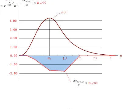
Fig.1 (1) is the graph of

N N

i i u

u~ )

( 1



×

D

0o

(

u

)

⊿

u

~

u

,

the real contributions

of thermal electrons of



= 0

o

, and of different speed ranges

⊿

_u

_.

Fig. 1(2) Graph of the actual contributions of electrons of  = 0o and of

different speeds,

N N

i i u

u~ ) ( 1



×D0o (u) ~ u and

N N

i i u

u~ ) ( 1



×D0o(u)⊿

u ~

u.

(29)

the output current of all the vertically emitted electrons from A and B

is not zero. It is positive

.

This is sharply in contradiction to

Boltzmann’s principle of detailed balance.

(30)

The Second Part of the survey

Trajectories of thermal electrons of other

exiting

angles (

≠

0

o

_{) and of different speeds}

The following exiting angles and speeds are adopted

 = -15

o

_{, 15}

o

_{, -30}

o

_{, 30}

o

_{, -45}

o

_{, 45}

o

_{, -60}

o

_{, 60}

o

_{, -75}

o

_{, 75}

o

u = 0.5u

p,

u

p,

1.5u

p,

2u

p,

2.5u

p,

3u

p,

3.5u

p,

4.5u

p.

(31)

2. Trajectories of electrons of = -15

o

_{and different speeds}

(1) Fig 2-1



= -15

o

_{u = 0.25u}

p

R = 1mm (B =1.34 gauss)

A-directly-A B-directly-B B-glass-B

(grey) CD/OF= 0.5/70 = 0.007≈0.01 No electron migration between A and B due to these trajectories.

A-directly-B B-Glass-A

(from MO to ON, MO = 9.5, red) (from G to H, etc., DF = 9, blue) MO/EO = 9.5/70 = 0.136 DF/OF= 9/70 = 0.129 A-B 13.6% of the electrons of (-15o, 0.25up) emitted from A migrate to B. B-A 12.9% of the electrons of (-15o_{, 0.25up) emitted from B migrate to A.}

For all the electrons of (-15o, 0.25up), migration A-B exceeds B-A, and their difference is the corresponding contribution to the output current

｛(A-B) – (B-A)｝-15o 0.25up = 0.136 – 0.129 = 0.007 D-15o(0.25up) = 0.007×cos15

o

(32)

(2)

Fig 2-2



= -15

o

_{u = 0.5u}

p

R = 2mm (

cos

-15

o





A-directly-A B-directly-B

B-Glass-B CD/OF=1/70 = 0.014 (grey) (CD = 1, OF =70) (green)

A-directly-B B-Glass-A

(from PO to OQ, red) (from J to K, etc., blue) (PO = 19, EO = 70) (DF = 18, OF = 70) 0 PO/EO = 19/70 = 0.27 DF/OF=18/70 = 0.26 A-B 27% of the electrons of (-15o, 0.5up) emitted from A migrate to B. B-A 26% of the electrons of (-15o, 0.5up) emitted from B migrate to A.

For all the electrons of (-15o, 0.5up), migration A-B exceeds B-A, and their difference is the corresponding contribution to the output current

｛(A-B) – (B-A)｝-15o 0.5up = 0.27 – 0.26 = 0.01 D-15o(0.5up) =｛(A-B) – (B-A)｝-15o 0.5up×cos15

o

(33)

(3)

Fig 2-3

= -15o

_{u = u}

p

R = 4mm (

cos

-15

o

= 0.9659)

A-directly-A B-directly-B

B-Glass-B (grey) CD/OF =2.5/70≈0.04 (green)

(CD=2.5, OF =70) No electron migration between A and B due to these trajectories.

(from P to O, M to N, O to Q, etc., red) (from G to H, D to L, etc., blue) (PO = 40, EO = 70) (DF = 37.5, OF = 70) PO/EO=40/70 = 0.57 DF/OF=37.5/70 = 0.54 A-B 57% of the electrons of (-15o, up) emitted from A migrate to B.

B-A 54% of the electrons of (-15o_{, up) emitted from B migrate to A.}

For all the electrons of (-15o, up),A-B exceeds B-A, and their difference is the corresponding contribution to the output current.

｛(A-B) – (B-A)｝-15oup= 0.57 – 0.54 = 0.03 D-15o(up) = 0.03×cos15

o

(34)

(3)

Fig 2-4



= -15

o

_{u = 1.5u}

p

R = 6mm

A-glass-A A-directly-A B-directly-B B-Glass-B

(brown) (grey) (grey) CD/OF = 5/70 =0.07 (green) No electron migration between A and B due to these trajectories.

A-directly-B B-glass-A

(from PMO to ONQ, PO = 58, red) (from G to H, etc., blue, DF = 54) PO/EO=58/70 = 0.83 DF/OF=54/70 = 0.77 A-B 83% of the electrons of (-15o, 1.5up) emitted from A migrate to B. B-A 77% of the electrons of (-15o, 1.5up) emitted from B migrate to A.

For all the electrons of (-15o_,_1.5up), _migration _{A-B exceeds} _{B-A, and their}

difference is the contribution to the output current,

｛(A-B) – (B-A)｝-15o1.5up = 0.83 – 0.77 = 0.06 D-15o(1.5up) =｛(A-B) – (B-A)｝-15o 1.5up×cos15

o

(35)

(4)

Fig 2-5



= -15

o

_{u = 2u}

p

R = 8mm

A-directly-B A-glass-B (from MP to NQ, red. MP=58, EO=70) (EM=2.5, PO=9.5, violet) 58/70 = 0.83 12/70 = 0.17 EM + MP + PO = 70

70/70 =1.00

A-B 100% of the electrons of (- 15o, 2up) emitted from A migrate to B.

B-glass-A

(from G to H, etc., blue, OE = 70) 70/70 = 1.00

B-A 100% of the electrons of (-15o_{, 2up) emitted from B migrate to A.}

For all the electrons of (-15o, 2up), migration A-B equals B-A, no net contribution to the output current,

｛(A-B) – (B-A)｝-15o 2up = 1.00 -1.00 = 0

D-15o(2up) = ｛(A-B) – (B-A)｝ -15o 2up×cos15

o

(36)

(6)

Fig 2-6



= -15

o

_{u = 2.5u}

p

R = 10mm

A-directly-B (red) A-glass-B (violet + volet) A-B = A-glass-B + A-directly-B + A-glass-B (violet + red + violet = 70) 70/70 = 1.00 A-B 100% of the electrons of (-15o_{, 2.5up) emitted from A migrate to B.}

B-Glass-A

(from G to H, F to J, O to L, etc., blue) 70/70 = 1.00

B-A 100% of the electrons of (-15o, 2.5up) emitted from B migrate to A.

For all the electrons of (-15o, 2.5up), migration A-B equals B-A, and their contribution to the output current cancel each other.

(A-B) – (B-A)｝ -15o 2.5up = 1.00 -1.00 = 0

D-15o (2.5up) =｛(A-B) – (B-A)｝-15o 2.5up×cos15

o

(37)

(7)

Fig 2-7



= - 15

o

_{u = 3u}

p

R = 10mm

A-glass-B (from M to N, etc., red) 70/70 = 1.00

A-B 100% of the electrons of (-15o, 3up) emitted from A migrate to B.

B-Glass-A (from G to H, etc., blue) 70/70 = 1.00

B-A 100% of the electrons of (-15o, 3up) emitted from B migrate to A.

For all the electrons of (-15o, 3up), migrations A-B and B-A cancel each other, no net contribution to the output current,

｛(A-B) – (B-A)｝-15o 3up = 1.00 -1.00 = 0 D-15o(3up) =｛(A-B) – (B-A)｝-15o3up×cos15

o

= 0

(38)

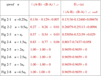
Every 100 + 100 electrons (1.00 = 100% from A, 1.00 = 100% from B)

of exiting angle



= -15

o

and of different speeds contribute to the electron

migration between A and B differently, as list in Tab 2 (1) (

cos

-15

o

₌

0.9659)

,

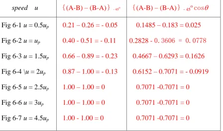
speed u

﹛

(A-B) - (B-A)

﹜

-15o

D

-15o

(

u

)

﹛

(A-B) - (B-A)

﹜

-15o cos

Fig 2-1

u =0.25u

p

Fig 2-2

u

= 0.5u

p

Fig 2-3

u = u

p

Fig 2-4

u = 1.5u

p

Fig 2-5

u = 2u

p

Fig 2-6

u = 2.5u

p

Fig 2-7

u = 3u

p

Fig 2-8

u =4.5u

p

0.136 – 0.129= 0.007

0.27 – 0.26 = 0.01

0.57 – 0.54 = 0.03

0.83 – 0.77 = 0.06

1.00 – 1.00 = 0

1.00 - 1.00 = 0

0.13136-0.12460=0.00676

0.26079-0.25113 =0.0096

0.55056-0.52159 =0.029

0.8017-0.7437=0.058

0.9659-0.9659 = 0

(39)

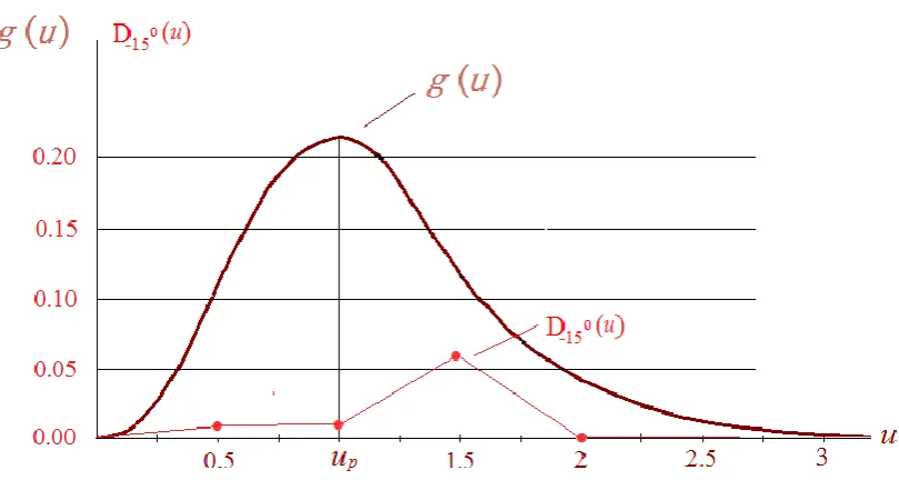
And Fig 2(1) is the corresponding graph.

(40)

Take Maxwell speed distribution

g

(u)

into account to derive the actual

contributions of the thermal electrons of



= -15

o

and of different speed

ranges, as list in Tab 2 (2),

N N

i i v

v~ ) ( 1



×

_D

_-15o

(

u

)

⊿

_u

_~

_u

_.

Speed range

⊿

u

N

i i u

u ~ )

( _₁



_D

_-15o

(

u

)

₌

﹛

(A-B)-(B-A)

﹜

-15o cos

N N

i i u

u~ ) ( 1



×

D

-15o

(

u

)

⊿

u

0.00~0.25u

p

0.25~0.75u

p

0.75~1.25u

p

1.25~1.75u

p

1.75~2.25u

p

2.25~2.75u

p

2.75~3.25u

p

3.25~3.75u

p

3.75u

p

~

∞

A0

≈ 0.004

A1

= 18.74%

A2

= 39.83%

A3

= 26.71%

A4

= 8.82%

A5

= 1.58%

A6

= 0.16%

A7

=

0.0096%

A8

=

0.0003%

0.1314-0.1246=0.0068

0.26079-0.25113=0.0096

0.55056-0.52159=0.029

0.8017-0.7437=0.058

0.9659-0.9659 = 0

.00052-0.000498=0.00002

4.8874-4.7056 = 0.1818

21.9304-20.7753 = 1.1551

21.5576-19.8642 = 1.6934

8.5192 - 8.9152 = 0

1.5261 – 1.5261 = 0

0.1545 – 0.1545 = 0

0.00927 -0.00927 = 0

0.00029-0.00029 = 0

∑

u

N N

i i u

u~ ) ( 1



×

D

-15o

(

u

)

⊿

u

= 58.5852 – 55.9509 = 2.6343

(41)

The corresponding graph of

N N

i i u

u~ ) ( 1



×

D

-15o

(

u

)

~

u

is shown in Fig

2 (2).

Fig 2 (2) Graph of

N N

i i u

u~ ) ( _₁ 

(42)

3. Trajectories of electrons of



= 15

o

and different speeds

(1) Fig 3-1



= 15

o

_{u= 0.5u}

p

R = 2mm (B =1.34 gauss)

A-directly-A & B-directly-B B-glass-B 2.5/70=0.0357 (grey) (from CD to FV, CD=2.5, OF=70) No electron migration between A and B due to these trajectories.

(from MO to ON, red, MO=19, EO=70) (from D to H, etc. blue) (DF=16.5, OF=70) 19/70 = 0.271 16.5/70 = 0.235

A-B 27% of the electrons of (15o, 0.5up) emitted from A migrate to B. B-A 23.5% of the electrons of (15o, 0.5up) emitted from B migrate to A.

﹛(A-B) - (B-A)﹜15o 0.5up = 0.271 – 0.235 = 0.036 ≈ 0.04

(43)

(2) Fig 3-2





= 15

o

_{u = u}

p

R = 4mm (

cos

15

o





A-directly-A & B-directly-B B-glass-B No electron migration between A and B due to these trajectories.

A-directly-B B-glass-A (from PO to OQ, etc., red) (from G to H, etc., blue) PO/EO = 39/70 = 0.56 (PO=39) DF/OF = 33.7/70 = 0.48 (DF=33.7) A-B 56% of the electrons of (15o, up) emitted from A migrate to B.

B-A 48% of the electrons of (15o, up) emitted from B migrate to A.

For all the electrons of (15o_{, up),}_{migration A-B exceeds B-A, and their difference is}

the corresponding contribution to the output current

﹛(A-B) - (B-A)﹜15oup= 0.56 – 0.48 = 0.08

(44)

(3)

Fig 3-3



= 15

o

_{u = 1.5u}

p

R = 6mm

A-directly-A & B-directly-B

B-Glass-B

(from PO to OQ, red) (from G to H, D to K, etc., blue) PO/EO = 58/70 = 0.83 (PO=58) DF/OF = 47/70 = 0.67 (DF = 47)

A-B 83% of the electrons of (15o, 1.5up) emitted from A migrate to B. B-A 67% of the electrons of (15o, 1.5up) emitted from B migrate to A.

For all the electrons of (15o_{, up),}_{migration A-B exceeds B-A, and their difference is}

the corresponding contribution to the output current

﹛(A-B) - (B-A)﹜15o1.5up = 0.83 – 0.67 = 0.16

(45)

(4)

Fig 3-4



= 15

o

_{u = 2u}

p

R = 8mm

A-directly-B 64/70 = 0.91 A-glass-B 6/70 = 0.09 (from E to Q, M to N, P to F, red) (from PO to FS, violet) A-B = A-directly-B + A-glass-B (64 + 6 =70, red + violet) 70/70 = 1.00 A-B 100% of the electrons of (15o_{, 2up) emitted from A migrate to B.}

B-glass-B B-glass-A

(from O to U, D to V, etc., green) (from D to J, G to H, etc., blue) No electron migration DF/OF=59.5/70 = 0.85 B-A 85% of the electrons of (15o, 2up) emitted from B migrate to A.

For all the electrons of (15o, 2up),migration A-B exceeds B-A, and their difference is the corresponding contribution to the output current

﹛(A-B) - (B-A)﹜15o2up= 1.00 – 0.85 = 0.15

(46)

(5)

Fig 3-5



= 15

o

_{u = 2.5u}

p

R = 10mm

A-directly-B (45/70) (red) A-glass-B (25/70) (violet) A-B (total) 70/70 = 1.00 (red +violet, 45 + 25 = 70 )

A-B 100% of the electrons of (15o, 2.5up) emitted from A migrate to B.

B-glass-B 1/70 = 0.014 B-glass-A (OD = 1, OF = 70) (DF = 69, OF =70) No electron migration between A (from G to H, etc., blue)

and B due to these trajectories. DF/OF = 69/70 = 0.986 B-A 98.6% of the electrons of (15o, 2.5up) emitted from B migrate to A.

For all the electrons of (15o_, _2.5up), _migration _{A-B exceeds} _{B-A, and their}

difference is the corresponding contribution to the output current

﹛(A-B) - (B-A)﹜15o2.5up = 1.00 – 0.986 = 0.014 D15o (2.5up) =﹛(A-B) - (B-A)﹜15o2.5up cos15

o

(47)

(6) Fig 3-6



= 15

o

_{u = 3u}

p

R = 12mm

A-directly-B A-glass-B

(from E to Q, M to N, P to F, etc., red) (from P to F, R to S, O to K, etc., violet) A-B (total) 70/70 = 1.00 (EP + PO = 20 + 50 = 70)

A-B 100% of the electrons of (15o_{, 3up) emitted from A migrate to B.}

B-glass-A

(from G to H, O to Q, etc., blue) 70/70 = 1.00

B-A 100% of the electrons of (15o, 3up) emitted from B migrate to A.

For all the electrons of (15o_{, 3up),}_{migration A-B equals B-A, and their contribution}

to the output current cancel each other.

﹛(A-B) - (B-A)﹜15o3up = 1.00 – 1.00 = 0

D15o(3up) = ﹛(A-B) - (B-A)﹜15o3up × cos15

o

(48)

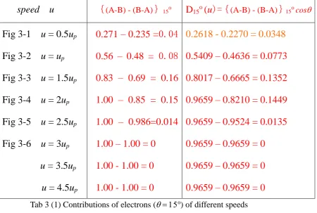
Every 100 + 100 electrons (1.00 = 100% from A, 1.00 = 100% from B)

of exiting angle



= 15

o

_{and of different speeds contribute to the electron}

migration between A and B differently, as list in Tab 3 (1) (

cos

15

o

=

0.9659)

,

speed u

｛

(A-B) - (B-A)

｝

15o

D

15o

(

u

)=｛

(A-B) - (B-A)

｝

15o cos

Fig 3-1

u = 0.5u

p

Fig 3-2

u = u

p

Fig 3-3

u = 1.5u

p

Fig 3-4

u = 2u

p

Fig 3-5

u = 2.5u

p

Fig 3-6

u = 3u

p

u = 3.5u

p

u = 4.5u

p

0.271 – 0.235 =

0.04 0.56 – 0.48 =

0.08 0.83 – 0.69 =

0.16 1.00 – 0.85 = 0.15

1.00 – 0.986=0.014

1.00 – 1.00 = 0

1.00 - 1.00 = 0

0.2618 - 0.2270 = 0.0348

0.5409 – 0.4636 = 0.0773

0.8017 – 0.6665 = 0.1352

0.9659 – 0.8210 = 0.1449

0.9659 – 0.9524 = 0.0135

0.9659 – 0.9659 = 0

Tab 3 (1) Contributions of electrons (o) of different speeds

Fig 3 (1) is the corresponding graph.

(49)

Take Maxwell’s speed distribution

g

(

u

)

into account to derive the

actual contributions of the thermal electrons of



= 15

o

and of different

speed ranges, i.e.,

N N

i i u

u~ )

( 1



×

D

15o

(

u

)

⊿

u

~ u, as shown in table 3(2).

Speed range

⊿

u

N N₍_u_i_~_u_i_₁₎



_｛

_(A-B)-(B-A)_﹜₁₅o _cos

N N₍_u_i_~_u_i_₁₎ 

×

D

15o

(

u

)

⊿

u

0.00~0.25u

p

0.25~0.75u

p

0.75~1.25u

p

1.25~1.75u

p

1.75 ~ 2.25u

p

2.25 ~ 2.75u

p

2.75 ~ 3.25u

p

3.25~3.75u

p

3.75u

p

~

∞

A0

≈ 0.004

A1

= 18.74%

A2

= 39.83%

A3

= 26.71%

A4

= 8.82%

A5

= 1.58%

A6

= 0.16%

A7

=

0.0096%

A8

=

0.0003%

0.2618-0.2270= 0.0348

0.5409–0.4636=0.0773

0.8017–0.6665=0.1352

0.9659–0.8210=0.1449

0.9659–0.9524=0.0135

0.9659 – 0.9659 = 0

0.0011-0.0009=0.0002

10.1365-8.6879=1.4486

31.9317-26.5466=5.3851

25.7992-21.9289=3.8703

8.5192-8.4002=0.1190

1.5261-1.5261= 0

0.1545-0.1545= 0

0.0093-0.0093=0

0.00029-0.00029=0

∑

u N N i i u

u~ )

( 1



×

D

15o

(

u

)

⊿

u

= 78.0799-67.2541=10.8232

(50)

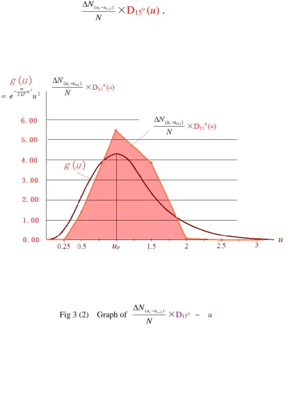
Fig 3 (2) is the corresponding graph

N N

i i u

u~ )

( 1



×

_D

15o

(

u

)

.

Fig 3 (2) Graph of N N

i i u

u~ )

( 1



×D15o ~ u

(51)

4. Trajectories of electrons of



=

- 30

o

_{and different speeds}

(1) Fig 4-1  = - 30o u = 0.5up R = 2mm (B = 1.34 gauss)

A-directly-A B-directly-B B-glass-B 1/70 = 0.014 (green) (grey) (CD = 1, OF =70) (from CD to UV) No electron migration between A and B due to these trajectories.

A-directly-B B-Glass-A (from PO to OQ, red) (from G to H, etc., blue)

(PO = 16.5, EO = 70) (DF =18, OF = 70) 16.5/70 = 0.236 18/70 = 0.257 A-B 24% of the electrons of (- 30o, 0.5up) emitted from A migrate to B. B-A 26% of the electrons of (- 30o_{, 0.5up) emitted from B migrate to A.}

For all the electrons of (-30o, 0.5up),migration A-B is less than B-A, and their difference is the corresponding contribution to the output current (negative).

﹛(A-B) - (B-A)﹜-30o0.5up = 0.236 - 0.257 = - 0.021

(52)

(2)

Fig 4-2



=

- 30

o _{u =}

_u

p

R = 4mm (

cos

-30

o





A-glass-A A-directly-A B-directly-B B-glass-B

(violet) (grey) (grey) CD/OF = 1.5/70 = 0.021 (green)

No electron migration between A and B due to these trajectories.

(PO =34) (from PO to OQ) (DF = 37) (from G to H, etc., blue) PO/EO = 34/70 = 0.49 DF/OF = 37/70 = 0.53

A-B 49% of the electrons of (- 30o, up) emitted from A migrate to B.

B-A 53% of the electrons of (-30o, up) emitted from B migrate to A.

For all the electrons of (-30o, up), migration A-B is less than B-A, and their difference is the corresponding contribution to the output current (negative).

(A-B) – (B-A)｝-30oup = 0.49 - 0.53 = - 0.04

(53)

(3)

Fig 4-3



=

- 30

o _{u =}

_1.5u

p

R = 6mm

(a) A-glass-A (green) + A-directly-A (grey)

(b) B-directly-B (c) B-glass-B (grey) (green)

(54)

(d) A-directly-B

(PO = 50, EO =70) (from PO to OQ, red) 50/70 = 0.71

A-B 71% of the electrons of (- 30o, 1.5up) emitted from A migrate to B.

(e) B-glass-A

(from G to H, J to K, etc., blue) (DF = 55, OF = 70) 55/70 = 0.79

For all the electrons of (-30o, 1.5up), migration A-B is less than B-A, their difference is the corresponding contribution to the output current (negative).

｛(A-B) – (B-A)｝-30o 1.5up = 0.71 - 0.79 = - 0.08

(55)

(4)

Fig 4-4



=

- 30

o _{u =}

_{2 u}

p

R = 8mm

A-glass-B + A-directly-B + A-glass-B violet red violet

70/70 =1.00

A-B 100% of the electrons of (-30o_{, 2up) emitted from A migrate to B.}

B-glass-A

(from G to H, K to L, F to X, etc. blue) 70/70 = 1.00

B-A 100% of the electrons (-30o, 2up) emitted from B migrate to A.

For all the electrons of (-30o, 2up), migration A-B and B-A cancel each other, no contribution to the output current.

｛(A-B) – (B-A)｝-30o 2up =1.00 -1.00 = 0

(56)

(5)

Fig 4-5



=

- 30

o _{u =}

_2.5u

p

R = 10mm

A-glass-B (red) 70/70 = 1.00

A-B 100% of the electrons of (-30o, 2.5up) emitted from A migrate to B.

B-glass-A (blue) 70/70 = 1.00

For all the electrons of (-30o, 2.5up), migration A-B and B-A cancel each other, no contribution to the output current.

(57)

Every 100 + 100 electrons (from A 1.00 = 100% and from B 1.00 =

100%) of exiting angle



= -30

o

_{and of different speeds contribute to the}

electron migration between A and B differently, as list in Tab 4 (1). Fig 4

(1) is the corresponding graph

(

cos

-30

o





D

-30o

(

u

)

=

｛

(A-B) – (B-A)

｝

 = -30o

cos



~

u

.

speed u

｛

(A-B) –(B-A)

｝

-30o

D

-30o

(

u

)



Fig 4-1

u =

0.5u

p

Fig 4-2

u =

u

p

Fig 4-3

u =

1.5u

p

Fig 4-4

u =

2u

p

Fig 4-5

u =

2.5u

p

Fig 4-6

u =

3u

p

0.235 - 0.257 = - 0.022

0.49 – 0.54 = - 0.04

0.71 - 0.79 = - 0.08

1.00 – 1.00 = 0

0.2035 – 0.2226 = - 0.0191

0.4243 – 0.4676 = - 0.0433

0.6149 – 0.6814 = - 0.0665

0866 – 0.866 = 0

Tab 4 (1) D-30o(u) =｛(A-B) – (B-A)｝ = -30ocos ~ u