Bilingual Lexicon Construction from Comparable Corpora via Dependency Mapping

Bilingual

Lexicon

Construction

from

Comparable

Corpora

via

Dependency

Mapping

QIAN Long Hua WANG Hong Ling ZHOU Guo Dong ZHU Qiao Ming*

NLP Lab, School of Computer Science and Technology Soochow University, Suzhou China 215006

{qianlonghua,hlwang,gdzhou,qmzhu}@suda.edu.cn

ABSTRACT

Bilingual lexicon construction (BLC) from comparable corpora is based on the idea that bilingual similar words tend to occur in similar contexts, usually of words. This, however, introduces noise and leads to low performance. This paper proposes a bilingual dependency mapping model for BLC which encodes a word’s context as a combination of its dependent words and their relationships. This combination can provide more reliable clues than mere context words for bilingual translation words. We further demonstrate that this kind of bilingual dependency mappings can be successfully generated and maximally exploited without human intervention. The experiments on BLC from English to Chinese show that, by mapping context words and their dependency relationships simultaneously when calculating the similarity between bilingual words, our approach significantly outperforms a state-of-the-art one by ~14 units in accuracy for frequently occurring noun pairs and similarly, though in a less degree, for nouns and verbs in a wide frequency range. This justifies the effectiveness of our dependency mapping model for BLC.

TITLE AND ABSTRACT IN ANOTHER LANGUAGE,CHINESE

应用依存映射从可比较语料库中抽取双语词表

从可比较语料库中抽取双语词表的基本思想是，双语相似的词语出现在相同的语词上下文 中。不过，这种方法引入了噪声，从而导致了低的抽取性能。本文提出了一种用于双语词 表抽取的双语依存映射模型，在该模型中一个词语的上下文结合了依存词语及其依存关 系。这种结合方法为双语词表构建提供了比单一的词语上下文更为可靠的信息。我们还进 一步展示了在没有人工干预的情况下可以产生和利用这种双语依存关系。从英文到中文的 双语词表构建实验表明，通过在计算双语词语相似度时同时映射词语及其依存关系，同目 前性能最好的系统相比，我们的方法显著提高了精度。对于经常出现的名词，精度提高了

14个百分点；对于较大频率范围内的名词和动词，性能也提高了，尽管程度较小。这说明

了依存映射模型对双语词表构建的有效性。

KEYWORDS: Bilingual Lexicon Construction, Comparable Corpora, Dependency Mapping

KEYWORDS IN CHINESE:双语词表构建,可比较语料库,依存映射

1 Introduction

Bilingual lexicons play an important role in many natural language processing tasks, such as machine translation (MT) (Och and Ney, 2003; Gong et al., 2011) and cross-language information retrieval (CLIR) (Grefenstette, 1998). Traditionally, bilingual lexicons are built manually with tremendous efforts. With the availability of large-scale parallel corpora, researchers turn to automatic construction from parallel corpora and achieve certain success (Wu and Xia, 1994). However, large-scale parallel corpora do not always exist for most language pairs. Therefore, researchers turn their attention to either pivot languages or non-parallel but comparable corpora.

Using pivot languages in BLC was pioneered by Tanaka and Umemura (1994). Thereafter, various studies have been done to take advantage of multiple paths (Mann and Yarowsky, 2001) and even multiple pivot languages (Mausam et al., 2009) between the source and target languages. Since such automatically constructed lexicons usually contain noisy and polysemous entries, corpus-based occurrence information has been widely used to help rank the candidate target words (Schafer and Yarowsky, 2002; Kaji et al., 2008; Shezaf and Rappoport, 2010).

Alternatively, extracting bilingual lexicons from comparable corpora assumes that words with similar meanings in different languages tend to occur in similar contexts, even in non-parallel corpora. Rapp (1999) and Fung (2001) proposed a bilingual context vector mapping strategy to explore word co-occurrence information. Both studies rely on a large, one-to-one mapping seed lexicon between the source and target languages. Koehn and Knight (2002) investigated various clues such as cognates, similar context, preservation of word similarity and word frequency. Garera et al. (2009) proposed a dependency-based context model and achieved better performance than previous word-based context models. Recent studies concentrate on automatic augmentation of the seed lexicon either by extracting identical words between two closely related

languages (Ficšer and Ljubešić, 2011) or by aligning translation pairs from parallel sentences,

which is mined in advance from a comparable corpus (Morin and Prochasson, 2011). The problem with above method is that they only consider the words involved in the contexts and ignore other rich information therein, such as syntactic relationships, thus usually suffering from low performance especially when they are applied to two distinct languages such as English and Chinese. For example, our preliminary experiment with the dependency-based model (Garera et al., 2009) shows that English source word “profit” matches wrongly with Chinese target word

“企业” (enterprise), instead of the correct one “利润”, due to the higher similarity score with the

former than that with the latter. Further exploration shows that the word “企业” has a much

higher frequency than the word “利润” in the adopted corpus, thus tends to have a higher

similarity score due to richer (nevertheless noisy) contexts. We also find that some relevant

contextual words with both target words, such as “实现” (realize) and “成本” (cost) etc., share

the same or corresponding dependency relationships with “利润” (profit), i.e. dobj and conj, but

not with “企业” (enterprise).

bilingual contexts involving not only dependent words but also their relationships, and the similarity between bilingual words can be better calculated by considering the mappings of both context words and their relationships. Furthermore, while the mappings of bilingual words may suffer from the data sparseness problem due to the availability of only a small scale of given seed lexicon, the mappings of dependency relationships can be reliably generated from the seed lexicon without human intervention, making our method easily adapted to other language pairs and domains. Finally, the weights of different dependency mappings can be automatically learned using a simple yet effective perceptron algorithm.

The remainder of this paper is organized as follows. Section 2 reviews the related work. Section 3 introduces our comparable corpus and a strong baseline. Section 4 details our dependency mapping approach while the experimentation is described in Section 5. Finally, Section 6 draws the conclusion with future directions.

2 Related work

In this section, we limit the related work to BLC from comparable corpora between English and Chinese. For others, please refer to the general introduction in Section 1.

Due to distinct discrepancies between English and Chinese, BLC from comparable corpora between these two languages is challenging. Fung (2000) extracted word contexts from a comparable corpus, and calculated the similarity between word contexts via an online dictionary. Particularly she analyzed the impact of polysemous words, Chinese tokenization and English morphological information. Zhang et al. (2006) built a Chinese-English financial lexicon from a comparable corpus with focus on the impact of seed lexicon selection. Haghighi et al. (2008) proposed a generative model to construct lexicons for multiple language pairs, including English-Chinese, via canonical correlation analysis, which effectively explores monolingual lexicons in terms of latent matching.

In particular for BLC without any external lexicon, Fung (1995) focused on context heterogeneity in Chinese and English languages, which measures how productive the context of a word is, instead of its absolute occurrence frequency. She suggested that bilingual translation words tend to share similar context heterogeneity in non-parallel corpora. Specifically, she calculated the similarity between two bilingual words using the ratios of unique words in the right and left contexts. Yu and Tsujii (2009) proposed the notion of dependency heterogeneity, which assumes that a word and its translation should share similar modifiers and heads in comparable corpora, no matter whether they occur in similar contexts or not. In this sense, our approach is similar to theirs. However, while their distance measure of dependency heterogeneity is limited to three easily-mapping common relationships between two languages, namely SUB, OBJ and NMOD, we further generalize to automatic mappings of any bilingual dependency relationships. Another difference is that our method considers dependent words and their relationships simultaneously.

3 Corpus and baseline

3.1 Comparable corpus

In this paper, we generate a comparable corpus from the parallel Chinese-English Foreign Broadcast Information Service (FBIS) corpus, gathered from the news domain. This bilingual corpus contains about 240k sentences, 6.9 million words in Chinese and 8.9 million words in English. Similar to the way adopted in (Garera et al., 2009; Haghighi et al., 2008), we couple the first half of Chinese corpus and the second half on the English side as our comparable corpus. For corpus pre-processing, we use the Stanford POS tagger (Toutanova and Manning, 2000) and syntactic parser (Marneffe et al., 2006) to generate the POS and dependency information for each sentence in both Chinese and English corpora. Particularly, English words are transformed to their respective lemmas using the TreeTagger package (Helmut, 1994).

3.2 Bilingual lexicons for evaluation: seed, test and development

In the literature, different scales of bilingual seed lexicons have been used. For example, Rapp (1999) and Fung (2000) used large-scale dictionaries of 10-20k word pairs while other studies (Koehn and Knight, 2002; Haghighi et al., 2008; Garera et al., 2009) used only small dictionaries of about 100-1000 word pairs.

In this paper, we adopt a small scale one. In particular, we use the GIZA++ package (Och and Ney, 2000) to extract the most frequently occurring 1000 word pairs as the bilingual seed lexicon

(denoted as Ls) and the subsequent 500 noun pairs (denoted as LNt) as the primary bilingual test

lexicon. This way of generating the test lexicon for nouns has been commonly used in previous studies (Koehn and Knight, 2002; Haghighi et al., 2008; Garera et al., 2009). Besides, we frame a

secondary test lexicon (denoted as LAt) including 200 nouns, verbs and adjectives respectively,

which spread evenly in the four ranges of 1001-2000, 2001-3000, 3001-4000 and 4001-5000. The

goal of LAt is to evaluate the adaptability of our method to words with different categories in a

wide frequency range.

Different from other studies on context-based BLC which use the seed lexicon only for bilingual

word projection, we set aside a bilingual development lexicon Ld of nouns, verbs and adjectives

(denoted as LNd, LVd and LJd) respectively for fine-tuning our BLC system. This bilingual

development lexicon is constructed by randomly selecting 200 nouns, 200 verbs and 100

adjectives1 _{in the bilingual seed lexicon. Obviously we have}

s

As a state-of-the-art baseline, Garera et al. (2009) extracted the words from the dependency tree

with a fixed window size of ±2 as the context. That is, given a word w in a sentence, all the words

corresponding to its immediate parent (-1), immediate children (+1), grandparent (-2) and grandchildren (+2) are extracted as features to constitute a context vector. Specifically, each

feature in the vector is weighted by its point-wise mutual information (PMI) with the word w,

where N(w, c) is the co-occurrence frequency of word w and its context word c, N(w) and N(c)

are the occurrence frequencies of the words w and c respectively, N is the number of all word

occurrences in the corpus. Since PMI is usually biased towards infrequent words, we multiplied it with a discounting factor as described in (Lin and Pantel, 2002):

( , ) min( ( ), ( ))

( , ) 1 min( ( ), ( )) 1

N w c N w N c

N w c+ × N w N c +

(2)

Then, the pair-wise similarity scores between source word wsand candidate target words wt are

computed using the cosine similarity measure as follows:

( , ) ( , )

f f ∈L. We call Formula (3) the dependent word similarity as it is calculated solely on

dependent words in the contexts.

Finally, all the candidate target words are ranked in terms of their dependency word similarity

scores with source word ws, and the top one wˆt is selected as the translation word:

goal is to build a lexicon of nouns occurring frequently in the source text, one reasonable assumption is that their translation counterparts also occur frequently in the target text. Therefore,

in order to reduce the computation cost we limit the candidate words for source word ws,GEN w( s)

to the most frequently occurring nouns with the number set to 10 times of the size of the lexicon.

4 BLC via dependency mappings

In this section, we first present the dependency mapping model for BLC and then detail on how to manually and automatically generate dependency mappings via a given development lexicon.

4.1 Dependency mapping model

Following Garera et al. (2009) and Yu and Tsujii (2009), we further postulate that the mapping of dependency relationships can hold between two translation words in comparable corpora. It is worth noting that one dependency relationship in one language may not always be directly mapped to the same relationship in another language and there are even cases where one relationship may map to multiple relationships in another language (cf. Fig. 1).Generally, we can enumerate the mappings of dependency relationships between English and Chinese, either by crafting manually or generating automatically. Suppose that we already have such dependency

mappings between English and Chinese at hand, denoted as Ψ. Compared with the baseline

development lexicon LNd) with the relationship direction not considered. Formally, the weight of

each feature can be recast via PMI as:

2

where ct denotes the combination of the dependent word and its relationship. Similarly, this PMI

value is also discounted according to Formula (2).

Likewise, the dependency mapping similarity between source word ws and target candidate word

wt is calculated using the cosine similarity as follows:

( , ) ( , )

whose involved words are translation pairs in the seed lexicon and whose involved dependency

types are bilingually mapped in Ψ, i.e. ( .i , .i )

s t s

f word f word∈L and ( .i , i. )

s t

f type f type∈ Ψ.

Obviously, we can rank the candidate target words in terms of their dependency mapping similarity scores with the source word and select the top one as the translation word. However, this often leads to the data sparseness problem since the combination of a dependent word and its relationship occurs much less frequently than a dependent word alone. Therefore, the dependent word similarity and dependency mapping similarity are interpolated linearly for candidate ranking as follows:

( , ) ( , ) (1 ) ( , )

T s t DW s t DM s t

Sim w w = ×α Sim w w + −α ×Sim w w (5)

Where Sim w wT( , )s t denotes the overall similarity score between the words ws and wt, and αis a

coefficient to balance these two similarity measures and can be fine-tuned using the development lexicon Ld.

4.2 Manually crafting dependency mappings

Considering the number of dependency relationships in both English and Chinese, e.g. 53 dependency relationships in Stanford encoding scheme, there are potentially thousands of possible mappings between these two languages. Fortunately, the distribution of various dependency relationships is severely skewed. Table 1 lists the statistics for the dependency relationships whose percentages are greater than 2% in the descending order, where the left three columns denote the English relationships, their short descriptions and percentages as well as the Chinese statistics on the right three columns. These statistics are obtained from 5000 most frequently occurring nouns in our English and Chinese corpora.

It shows that the top 8 types (prep, conj, nsubj, nn, amod, dobj, dep and poss for English and nn,

conj, dobj, assmod, nsubj, rcmod, amod and dep for Chinese) account for 87.2% and 94.2% of total dependency relationships for English and Chinese respectively. This means when we consider dependency mappings between English and Chinese, we can safely ignore other

relationships whose percentages are less than 2%. Furthermore, since the dep one in both English

specific ones, the mapping between dep and any other ones are not considered subsequently in

this paper.

EN Rel. Short Description % CN Rel. Short Description %

prep prepositional modifier 35.7 nn noun modifier 32.0

conj conjunction 11.8 conj conjunction 13.1

nsubj nominal subject 9.3 dobj direct object 11.8

nn noun modifier 8.6 assmod associative modifier 11.4

amod adjectival modifier 8.1 nsubj nominal subject 9.6

dobj direct object 7.6 rcmod relative clausal modifier 8.0

dep general dependency 3.6 amod adjectival modifier 4.5

poss possessive modifier 2.5 dep general dependency 3.8

Total 87.2 Total 94.2

TABLE 1 –Statistics on dependency relationships for English and Chinese nouns

Using linguistic knowledge from both English and Chinese languages, we manually craft 10

dependency mappings ΨM between these two languages, as shown in Fig. 1.

FIGURE 1 – Bilingual dependency mappings between English and Chinese

From the figure we can see that while some mappings, such as nsubj (EN) to nsubj (CN) and dobj

(EN) to dobj (CN), capture common grammatical relationships in both languages, others, such as

poss (EN) to assmod (CN), indicate the differences across the two languages. Particularly

interesting is that nn (CN) can map to four relationships, namely nn, amod, prep_of and poss (EN)

while nn (EN) has only one correspondence nn (CN). This indicates that nn (CN) is much more

productive and ambiguous than nn (EN). This scenario can be illustrated by possible mapping of

example Chinese phrase “中国银行” (nn) to English phrases “China Bank” (nn), “Chinese Bank”

(amod), “Bank of China” (prep_of) , and “China’s Bank” (poss), though only the third is correct

while all the others are merely grammatically reasonable.

4.3 Automatically generating dependency mappings

While manually crafting dependency mappings between two languages do serve our purpose, its limitation exists in the need for bilingual knowledge and the lack of flexibility. One alternative is to automatically generate bilingual dependency mappings via a development lexicon. The idea behind is that not only the bilingual words with similar dependent words and dependency relationships tend to pair each other (cf. Section 4.1), but also the bilingual dependency relationships between similar dependent words and their context words tend to map to each other. Fig. 2 illustrates an algorithm to derive bilingual dependency mappings via a development lexicon.

In this figure, ΨA denotes the set of bilingual dependency mappings to be automatically

generated while Ds and Dt are the respective dependency mapping vectors for source word si and

Input: Ld={( , )}s ti i iN=1

Output: ΨA

Initialize: Ψ =A NULL

1. for i =1…N

2. extract Ds and Dt for si and ti 3. for each feature j

s

f and j t

f in Ds and Dt 4. if ( .j , j. )

s t s

f word f word ∈L then

5. add this mapping and its count to Ψ_A

6. end if 7. end for 8. end for

9. calculate the percentage for each mapping in ΨA

10. keep the top 30 most frequent mappings in ΨA

FIGURE 2 –Algorithm for automatically generating bilingual dependency mappings

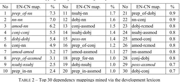
Table 2 shows the derived bilingual dependency mappings from English to Chinese along with their percentages. Compared with Fig. 1, we can see that all the 10 manually crafted mappings

(marked in italics fonts) in ΨM can be found in the top 30 automatically generated mappings ΨA,

with 8 in top 10. This implies high consistency between ΨA and ΨM. A natural question one may

ask is: are those extra mappings in ΨA but not in ΨM noisy for BLC?

No EN-CN map. % No EN-CN map. % No EN-CN map. %

1 prep_of-nn 7.3 11 nsubj-nn 1.7 21 prep_of-dobj 0.9

2 nn-nn 7.0 12 dobj-nn 1.6 22 nn-conj 0.9

3 amod-nn 6.2 13 conj-assmod 1.5 23 dobj-rcmod 0.8

4 conj-conj 5.5 14 nsubj-dobj 1.4 24 nsubj-assmod 0.8

5 dobj-dobj 5.4 15 poss-nn 1.4 25 amod-conj 0.8

6 conj-nn 4.9 16 prep_of-conj 1.2 26 amod-rcmod 0.8

7 amod-amod 3.2 17 amod-assmod 1.1 27 nn-assmod 0.8

8 prep_of-assmod 3.1 18 prep_for-nn 1.0 28 conj-dobj 0.8

9 nsubj-nsubj 2.5 19 dobj-nsubj 1.0 29 poss-assmod 0.7

10 prep_in-nn 2.4 20 prep_in-assmod 1.0 30 dobj-conj 0.7

TABLE 2 – Top 30 dependency mappings mined via the development lexicon

To answer this question is by no means a trivial task. Although we are quite sure that some of the

mappings in ΨA are irrelevant such as nsubj-assmod, for others it’s difficult to determine their

relevancy with BLC from the linguistic perspective, just as we are not sure whether there are

other useful mappings missing in ΨM. Therefore, we adopt an ablation testing strategy to

progressively remove those mappings whose removal lead to better performance using the

development lexicon Ld. Fig. 3 illustrates the algorithm, where Pi in Line 2 denotes the

performance achieved on the development lexicon Ld using previous mappings ΨiA−1 and Pj in

Line 4 denotes the performance on Ld using mappings Ψ_Ai−1 minus the jth mapping. The output of

Input: ΨA and Ld

FIGURE 3 –Algorithm for filtering the noisy mappings in ΨA

4.4 Weight learning via perceptron

While coefficient α in Formula (5) can be determined empirically using a development lexicon,

it equally weighs different mappings. We argue that this may not be optimal since different mappings may have different contributions to BLC. That is, different mappings should have different weights to exploit such difference. Thus, Formula (5) can be recast as follows:

)

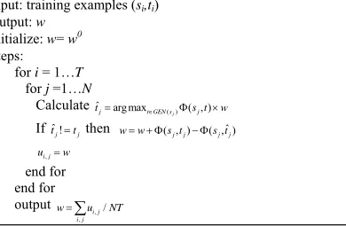
In this paper, we propose a simple perceptron algorithm to optimize those weights for different mappings using the development lexicon. Generally, the perceptron algorithm is guaranteed to find a hyper-plane that classifies all training points, if the data is separable. Even the data is non-separable as in most practical cases, the variants of perceptron (Freund and Schapire, 1999; Collins and Duffy, 2002), such as averaged perceptron (AP) or voted perceptron (VP), can generalize well.

Fig. 4 shows our averaged perceptron algorithm, where

occurrence ratio for each mapping as in Table 2.

Here, the function Φ calculates the dependent word similarity score (cf. Formula (3)) and the

similarity scores for each dependency mapping in Ψ (cf. Formula (3’)), ui,j stores the weight

vector in the ith iteration given the jth training example, and T denotes the number of iterations

over the development lexicon2_.

5 Experimentation

This section systematically evaluates our approach for English-Chinese BLC. In this paper, precision (P) and mean reciprocal rank (MRR) are used as our evaluation metrics, as done in the literature (Koehn and Knight, 2002; Garera et al., 2009; Yu and Tsujii, 2009), where precision is

the average accuracy within the top n (n=1 here) most similar words while MRR is the average of

the reciprocal ranks for all the test words:

w

count is the number of correct translation words on the top one ranking, and ranki

denotes the rank of the correct translation word for the ith test source word, and

w

N is the total

number of the test source words (e.g., 500).

5.1 Performance on the development noun lexicon LNd

In order to determine the optimal subsets in automatic mappings ΨA and manual mappings ΨM

respectively, we conduct ablation tests on the development lexicon LNd (cf. Fig. 3) using

proportional weights (PR) or automatic weights learned by the AP algorithm (cf. Fig. 4). Fig 6 depicts the MRR performance scores for 4 combinations, i.e. Auto-PR, Auto-AP, Manual-PR and

Manual-AP. For ΨA, x-axis denotes the top 30 mappings (cf. Table 2) while for ΨM we present

the data from the 20th iteration as there are only 10 mappings (cf. Fig. 1). At each iteration, the mapping whose removal causes the biggest performance increase is removed and the MRR score is measured using the remaining mappings. The integer numbers in Table 2 indicate the mappings to be removed at the corresponding iteration. Please note that the first iteration

corresponds to all dependency mappings in ΨA or ΨMand the last one corresponds to the baseline

without any dependency mapping. The figure shows that:

30

¾The dependency mapping model with average perceptron significantly outperforms its

counterpart with proportional weights. This suggests that weight optimization via perceptron algorithms substantially helps BLC. Therefore, the following experiments do not consider proportional weights.

¾All the 4 combinations exhibit similar trends. That is, with the shrinkage of the mappings, the

performance first slightly increases, then peaks at some iteration, afterwards decreases slowly, and finally drops significantly. This trend suggests that there do exist some noisy mappings,

more or less in both ΨA and ΨM. However, removing them can only lead to limited

performance improvement while too few mappings severely harm the performance.

¾An interesting phenomenon is that the two combinations (Auto-AP and Manual-AP) converge

at the last 7 iterations, so do the other two (Auto-PR and Manual-PR). This implies high consistency between manually crafted mappings and top automatically generated mappings no matter whether their weights are fine-tuned using a proper machine learning algorithm or fixed to their proportions in the corpus.

According to above observations, we select the most consistent mappings as the optimal ones in all the following experiments instead of choosing the best mappings for each combination. These

sets, marked by the symbols o

A

Ψ (15 mappings for Auto_AP) and o

M

Ψ (8 mappings for

Manual_AP) in the figure, include medium-sized mappings which perform the best or very

closely to the best. It is not surprising to find that 7/8 mappings in o M

Ψ are included in o

A

Ψ

because of their high consistency.

5.2 Comparison of mapping weights in o A Ψ and o

M Ψ

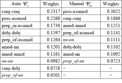
Table 3 ranks the weights learned for each mapping in o

A

Ψ and o

M

Ψ in the descending order,

where the mappings with negative weights are omitted. It shows that different mappings have

very different weights, among which conj-conj and poss-assmod are ranked high while nn-nn and

prep_of-nn are ranked low. This suggests that the former two are more discrimitive than the latter

two in dependency mapping-based BLC, though the latter two occur more frequently as indicated in Table 2. In other words, the meaning of a noun depends more on its conjuncts and possessive/associative modifiers to a certain extent than on its prepositional phrases or noun premodifers.

conj-conj 0.2317 poss-assmod 0.3022

poss-assmod 0.2268 conj-conj 0.1866

prep_in-assmod 0.1738 amod-amod 0.1251

dobj-dobj 0.1597 prep_of-assmod 0.1141

prep_of-assmod 0.1264 nn-nn 0.1111

amod-nn 0.1201 dobj-dobj 0.1102

amod-amod 0.1161 amod-nn 0.1092

nn-nn 0.0982 prep_of-nn 0.0723

conj-dobj 0.0758 - -

5.3 Performance on the test noun lexicon LNt

Table 4 shows the performance of our dependency mapping model (DM) on the test noun lexicon

LNt. Three weighting strategies, i.e. DM (equal weights), DM_PR (proportional weights) and

DM_AP (weight learning by the AP algorithm on LNd) are used with four sets of dependency

mappings (

Ψ ). Please note that all the optimal mappings are tuned on the

development lexicon as discussed in Fig. 6, though we don’t present the results of ablation tests for DM there as they are similar to those of DM_PR. For comparison, the strong baseline as discussed in Section 3 is included at the top row. The table shows that:

¾ The AP3 _{algorithm (DM_AP) achieves the best performance with the improvements of ~6}

units in P and ~5 in MRR compared with DM. In most cases, DM_PR slightly underperforms DM, which means that simply using the occurrence ratio as each mapping’s weight doesn’t lead to performance improvement.

¾ In total, our method outperforms the strong baseline by ~14 units in both P and MRR

across all the mapping sets. This suggests that via weight learning with a proper machine

learning method (e.g. a simple perceptron algorithm), the dependency mapping model can dramatically improve the performance for BLC.

¾ A particularly important finding is that the optimal automatic mapping set o

A

Ψ performs

comparably with the manual mapping set Ψ_Mand slightly outperforms the complete

automatic mapping set Ψ_A. This further justifies the appropriateness of automatically

generating bilingual dependency mappings.

DM DM_PR DM_AP

Systems

P (%) MRR(%) P (%) MRR(%) P (%) MRR(%)

Baseline 33.8 42.23 33.8 42.23 33.8 42.23 Manual

M

Ψ 43.0 51.89 42.4 51.61 49.2 57.18

Manual o

M

Ψ 44.0 52.44 40.2 49.52 50.0 57.62

Auto Ψ_A 41.4 50.70 39.0 48.64 46.2 55.50

Auto o

A

Ψ 42.6 51.66 43.6 51.85 48.6 56.43

TABLE 4 – Performance of dependency mapping on the test noun lexicon LNt

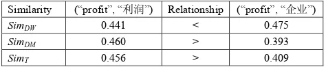
Above observations justifies that dependency mappings can significantly enhance the performance for BLC, and perform even better when the weight for each mapping is optimized. To explain how dependency mappings work, we take English word “profit” and its Chinese

translation “利润” as an example, which is also mentioned in Section 1. Table 5 compares three

kinds of similarity scores between “profit” and its two translation candidates, i.e., “利润” and “企

业”. It shows that due to SimDM (“profit”, “利 润”) >SimDM (“profit”,“企 业”), our method

eventually acquires the correct translation pair of “profit” and “利润”. The reason is that the

dependency mapping context between “profit” and “利润”, such as “实现_dobj” (realize_dobj)

and “成本_conj” (cost_conj) etc., is more evidential than that between “profit” and “企业”. In

other words, the dependency mapping context contains more accurate bilingual corresponding words and ignores noisy ones than the dependent word context, thus leading to better performance for BLC.

Similarity (“profit”, “利润”) Relationship (“profit”, “企业”)

SimDW 0.441 < 0.475

SimDM 0.460 > 0.393

SimT 0.456 > 0.409

TABLE 5 – Similarity comparison between “profit” and its two translation candidates

5.4 Performance on the general test lexicon LAt

Table 6 compares the performance of different methods on the general test lexicon LAt for words

with different categories (i.e. nouns, verbs and adjectives) in a wide frequency range. Specifically, for the DM and DM_AP methods, the automatic mappings and their weights for nouns are the same as those in Table 2 while for verbs and adjectives, the mappings are first automatically generated and then filtered using the ablation tests with their weights learned on the development

¾ For nouns and verbs, both the DM and DM_AP methods with automatic dependency mappings outperform the baseline, though with the improvements in a less degree than

those for nouns in LNt, due to the much more data sparseness of both the dependent word

context and dependency mapping context.

¾ For adjectives, however, the performances of three methods are quite similar. This

suggests the non-effectiveness of dependency mappings on BLC for adjectives.

Baseline DM DM_AP

Parts of speech _{P(%) MRR(%) P(%) MRR(%) P(%) MRR(%)}

Nouns 21.8 28.62 26.0 33.60 28.3 35.02

Verbs 19.5 27.07 23.5 31.69 26.0 35.26

Adjectives 35.5 46.22 36.0 46.93 34.5 45.63

TABLE 6 – Performance of different methods on the general test lexicon LAt

Above observations demonstrate that our method can well adapt to nouns and verbs in a wide frequency range, but not to adjectives. Our exploration shows that, although the mappings for verbs are much different from those for nouns (cf. Table 2), both sets of mapping are diverse

without a dominant single mapping. However, for adjectives dependency mapping amod-amod

accounts for nearly 70% of total mappings. This reflects the fact that the dependency relationship between an adjective and its contextual words is much simpler than that for either a noun or a verb. The dominance of one mapping for adjectives makes the dependency mapping context highly correlated with the dependent word context, thus significantly weakens the effect of dependency mapping, while the diversity of dependency mappings for nouns and verbs ensures its efficacy.

Conclusion and perspectives

In this paper, we propose a bilingual dependency mapping model for bilingual lexicon construction from English to Chinese using a comparable corpus. When calculating the similarity between bilingual words, this model considers both dependent words and their relationships, thus

providing more accurate and less noisy representation. Evaluation shows that our approach

significantly outperforms a state-of-the-art baseline from English to Chinese on both nouns and verbs in a wide frequency range, though with the exception of adjectives. We also demonstrate that bilingual dependency mappings can be automatically generated and optimized without human intervention, leading to a medium-sized set of dependency mappings, and that their contributions on BLC can be fully exploited via weight learning using a simple yet effective perceptron algorithm, making our approach easily adaptable to other language pairs.

In future work, we intend to apply our method to BLC between other language pairs. Preliminary experiments show that the dependency mapping model can improve the precision for BLC by ~6 units from Chinese to English.

Acknowledgments

References

Collins, M., and Duffy, N. (2002). New Ranking Algorithms for Parsing and Tagging: Kernels over Discrete Structures, and the Voted Perceptron. ACL’2002.

Ficšer. D. and N. Ljubešić. (2011). Bilingual Lexicon Extraction from Comparable Corpora for

Closely Related Languages. RANLP’2011: 125–131.

Fung, P. (1995). Compiling bilingual lexicon entries from a non-parallel English-Chinese corpus. In the Third Annual Workshop on Very Large Corpora: 173–183.

Fung, P. (2000). A statistical view on bilingual lexicon extraction: from parallel corpora to nonparallel corpora. In the Third Conference of the Association for Machine Translation in the Americas.

Freund, Y. and Schapire, R. E. (1999). Large margin classification using the perceptron algorithm. Machine Learning, 37(3): 277-296.

Garera, N., Callison-Burch, C., and Yarowsky, D. (2009). Improving translation lexicon induction from monolingual corpora via dependency contexts and part-of-speech equivalences. CoNLL’2009: 129–137.

Gong Z. X., Zhang M. and Zhou G. D. (2011). Cache-based document-level statistical machine translation. EMNLP’2011:909-919.

Grefenstette, G. (1998). The Problem of Cross-language Information Retrieval. Cross-language Information Retrieval. Kluwer Academic Publishers.

Haghighi, A., Liang, P., Berg-Krikpatrick, T., and Klein, D. (2008). Learning bilingual lexicons from monolingual corpora. ACL’2008: 771–779.

Helmut, S. (1994). Probabilistic part-of-speech tagging using decision trees. In Proceedings of the International Conference on New Methods in Language Processing (NeMLaP): 44–49. Kaji, H., Tamamura, S. and Erdenebat, D. (2008). Automatic construction of a Japanese-Chinese dictionary via English. LREC’2008: 699–706.

Koehn, P. and Knight, K. (2002). Learning a translation lexicon from monolingual corpora. In Proceedings of ACL Workshop on Unsupervised Lexical Acquisition.

Lin, D. and Pantel, P. (2002). Concept Discovery from Text. COLING’2002: 42–48.

Mann, G. S., and Yarowski, D. (2001). Multipath translation lexicon induction via bridge languages. NAACL’2001: 151-158.

Marneffe, M.-C. de, MacCartney, B., and Manning, C. D. (2006). Generating typed dependency parses from phrase structure parses. LREC’2006.

Mausam, S. Soderland, O. Etzioni, D. S. Weld M. Skinner, and J. Bilmes. (2009). Compiling a Massive, Multilingual Dictionary via Probabilistic Inference. ACL’2009: 262–270.

Och, F. J. and Ney, H. (2000). Improved Statistical Alignment Models. ACL’2000: 440-447.

Och, F. J. and Ney, H. (2003). A Systematic Comparison of Various Statistical Alignment Models. Computational Linguistics, 29(1): 19-51.

Rapp, R. (1999). Automatic identification of word translations from unrelated English and German corpora. ACL’99: 519–526.

Schafer, C. and Yarowsky, D. (2002). Inducing Translation Lexicons via Diverse similarity Measures and Bridge Languages. CoNLL’2002.

Shezaf, D. and Rappoport, A. (2010). Bilingual Lexicon Generation Using Non-Aligned Signature. ACL’2010: 98–107.

Tanaka, K. and Umemura, K. (1994). Construction of a bilingual dictionary intermediated by a third language. COLING’94: 297-303.

Toutanova, K. and Manning, C. D. (2000). Enriching the Knowledge Sources Used in a Maximum Entropy Part-of-Speech Tagger. EMNLP/VLC’2000: 63-70.

Wu, D. and Xia, X. (1994). Learning an English-Chinese Lexicon from a Parallel Corpus. In Proceedings of the 1st Conference of the Association for Machine Translation in the Americas.

Yu, K. and Tsujii, J. (2009). Extracting bilingual dictionary from comparable corpora with dependency heterogeneity. NAACL-HLT’2009: 121–124.