Two Server Queuing Systems Reaches its Capacity in Time t*

(1)

417

Two Server Queuing Systems Reaches its

Capacity in Time t

*

Dhanesh Garg

School of Mathematics and Computer Applications, Thapar University, Patiala-147004, India,

E-mail: [email protected]

Abstract: This paper presents a simple and computing the joint probability distribution of the number of

customers and the number of times system reaches its capacity in time t with homogeneous servers of M/M/2/N

Keywords: Transient analysis, Homogeneous servers, Finite capacity.

1. INTRODUCTION:

In the last one decade a lot of work has been done by various authors taking into consideration the concept of transient (time dependent) behavior of queueing systems. Transient solutions for queueing systems are normally assumed to be an intractable problem with practical interest. However, there are cases where transient behavior is important or even more importantly, steady state values provide insufficient information regarding the system performance. For instance, in the evaluation of high speed broadband networks, new performance measures such as interval-based quality of service measures require transient analysis [2]. In all the mentioned studies the researchers have obtained the state probabilities in one way or the other and have computed various measures of performance. In this paper we have explicitly obtained the joint probability distribution of the number of times the system reaches its capacity in time t with two homogeneous servers. Also this paper is the particular case of [5*], no catastrophic occurs. The rest of paper is organized as follows. In section 2 model is described and analyzed. Section 3, the number of times system reaches its capacity in time t. Section 4, conclusion.

2. MODEL DESCRIPTION AND ANALYSIS:

We consider an M/M/2/N queueing system having two homogenous servers with FCFS discipline subjected to catastrophe. The customers arrive at a counter in accordance with a Poisson process with mean arrival rate λ>0. Each server serves one customer at a time if available. The service time distribution of a customer

is negative exponential with mean rate µ>0. The queuing process starts at time zero with zero state of

the system. We

define

m, n

P

(t) = Prob. [X(t) = m, Y(t) = n], 0 n

≤ ≤

N

[2.1] Where X (t) = the number of times the system

reaches its capacity in time t. Y (t) = the number of customers in the system at time t. The marginal

probabilities are

., ,

0

( ) ( )

n m n

m

P t P t

∞

=

∑

and

,. ,

0

( ) ( )

N

m m n

n

P t P t

= =

∑

From these assumptions and by the forward Kolmogorov equations as follows:

,0

( )

,0

( )

,1

( )

m m m

d

P

t

P

t

P

t

dt

= −

λ

+

µ

[2.2]

, , , 1

, 1

( )

(

2 )

( )

2

( ) ;1

,

0

m n m n m n

m n

d

P

t

P

t

P

t

dt

P

t

n

N m

λ

µ

λ

µ

−

+

= − +

+

< <

≥

[2.3]

,1 ,1 ,0

,2

( )

(

)

( )

2

( ) ;

1,

0

m m m

m

d

P

t

P

t

P

t

dt

P

t

n

m

λ µ

λ

µ

= − +

+

=

≥

[2.4

,

( )

2

,

( )

1, 1

( )

m N m N m N

d

P

t

P

t

P

t

dt

= −

µ

+

λ

− −

[2.5] Taking Laplace transform of the equations [2.2]-[2.5] w.r.t t we have

0,0 0,1

(

s

λ

)

P

( )

s

1

µ

P

( ) ;

s

n

0,

m

0

− −

+

= +

=

[2.6]

,0 ,1

(

s

λ

)

P

m

( )

s

µ

P

m

( ) ;

s n

0,

m

0

− −

+

=

>

[2.7]

,1 _,0 ,2

(

s

λ µ

)

P

m

( )

s

λ

P

_m

( )

s

2

µ

P

m

( );

s n

1

− − −

+ +

=

+

=

(2)

418

, , 1 , 1

(

s

λ µ

2 )

P

m n

( )

s

λ

P

m n

( ) 2

s

µ

P

m n

( );2

s

n N

− − −

− +

+ +

=

+

≤ <

[2.9]

, 1, 1

(

s

2 )

µ

P

m N

( )

s

λ

P

m N

( );

s n

N

− −

+

=

[2.10] Since

P (0) = 1

_0,0

Where , _,

0

( )

st

( )

m n _{m n}

P

s

e

P

t dt

∞ −

−

=

∫

Define the probability generating functions by

, 0

( , )

( )

m

n m n

m

P x s

P

s x

∞

− −

=

∑

[2.11]

0

( , ; )

( , )

N

n n

n

H x y s

P x s y

− −

=

∑

[2.12]

. ,.

0

( , )

m

( )

m m

P x s

P

s x

∞

− −

=

∑

[2.13] Multiplying equation [2.6] to [2.10] by xm, summing over the ranges of m and using [2.11], we have

0 1

(

s

λ

)

P x s

( , ) 1

µ

P x s n

( , );

0

− −

+

= +

=

[2.14]

1 0 2

(

s

λ µ

)

P x s

( , )

λ

P x s

( , ) 2

µ

P x s

( , )

− − −

+ +

=

+

[2.15]

1 1

(

s

λ µ

2 )

P x s

n

( , )

λ

P

n

( , ) 2

x s

µ

P

n

( , )

x s

− − −

− +

+ +

=

+

[2.16]

1

(

s

2 )

µ

P

N

( , )

x s

λ

x P

N

( , );

x s n

N

− −

−

+

=

[2.17] Multiplying equation [2.14] to [2.17] by yn, summing over the ranges of n and using [2.12, 2.13], we have on simplification:

0

1 1

(1 )[2 ( )] ( , )

( 1)(2 )

( , )

(1 )

( 1)

2 ( , ; )

[ (1 )( 2 )]

N N

ys s y y s P x s

sy x y

P x s

x y

sy x

s H x y s

s sy y y

µ

λ

µ

λ

µ

−

− − +

−

− − + + +

− − +

 

 

 ₋ 

 _ _{− +} _  _ ₊ _

 

=

+ − −

[2.18]

Since,

( , )

1

( , )

2

N N

x

P

x s

P

x s

s

λ

µ

− −

−

=

+

The zeros of the denominator in [2.18] are given by

2

(

2 )

(

2 )

4 2

( )

,

1, 2.

2

i

s

i

λ

µ

λ

µ

λµ

α

λ

+ +

±

+ +

− ×

=

[2.19]

The existence of

H x y s

( , ; )

−

is only possible if numerator vanishes for α1 and α2 the two zeros of the

denominator. This will give rise two equations, solving them we have:

1 0

( , )

A x s

P x s

A x s

− −

−

=

[2.20]

2 1

(., )

( , )

N

A

s

P

x s

A x s

− −

−

=

₋ [2.21]

Where

{

}

{

}

1

( 1) ( ) 2

( , ) 2

(1 ) (1) ( )

x

V N V N

s A x s

x s V V N

λ µ µλ

− _ _ + − __

+

= _ _

_{+ −} _ ₋ _ 

 

[

]

2

(., )

2

(

2 )

(1)

A

s

µ

s s

λ

V

−

=

+

{

}

{

}

{

}

{

}

{

}

2

2 (1) ( 1) ( ) (1 )

( ) ( 1)

( , ) 2 ₍ ₂₎ ₍ ₁₎

( 1) ( ) 2

( ) ( ) ( 1)

V V N V N

x _s

V N V N

A x s s _{V N} _{V N}

x

s V N V N

s

s V N V N

γ

λ _γ

λ

µλ _λ _γ

γ µ

λ γ

−

  ₊ _{+ −}  

 ₋   

  ₊  

+ − −

 _ _ 

 

=   _{+ −} ₊ 

  

₊ ₊ _{+ −} 

 ₊  

 _{− +} ₋ ₋ 

 

[2

.18] Yields

0

1 1

1 2

0 1 0 2

[ ]

(1

)[2

(

)]

( , )

(

1)(2

)

( , )

(1

)

(

1)

2

(1)

N N

n n

y s

s

y

y s

P x s

sy x

y

P

x s

x

y

sy

x

s

s V

y

µ

λ

µ

λ

α

−

− − +

∞ ∞

− −

= =

−

+

−

− +











−







− +









+

























×





−



















∑



[2.22]

Now

P x s

n

( , )

−

is the coefficient of yn in [2.12]. Comparing the coefficients of yn on both sides of [2.22], we have:

2 2

0

{2

( )

(

)

( , )

(1)

(

1)}

( , )

( )

n

s T n

s s

P x s

s V

T n

P x s

sV n

µ γ

λ

γ

λ

−



+







=



−







(3)

419

{

}

{

}

2 0, 2

( )

(1)

2

( ) (

) (

1)

[ (1)

( )]

2

(1)

( )

(

) (

1)

n n

P

s

sV n

s V

T n

s

T n

s V

V N

V

T N

s

T N

γ

λ

µγ

λ

−

=

−



+ +

−







−









+

















+

−









[2.24] Applying the Leibniz differentiation theorem to [2.20], setting x=0 and dividing both sides by m!, we have:

{

}

{

}

2 2 1 2 2 ,0 ₁ 2

2 ( 2 ) (1) (1) ( ) ( 2 )

[( ) ( 1)

2 [( 2 ) (1)] [( ) 2 ( )] ( )

( 2 ) 2 (1) ( 1)

m

m _m

m m

s V

sV sV N s

s T N

s V

s s

P s

s s V T N

λγ µ

λ µ

γ

λγ µ

λ µ λ

γ µ λ

− − +   ₊     − − − +       ₋      _ ₊ _    _ _  __ ₊ ₊ ₊ __  =  + + −                   [2.25] 2 , ,0 2 ( ) ( ) ( ) (1)

2 ( ) ( ) ( 1)

n

m n m

P s P s sV n

s V

s T n

s s T n

γ λ µ γ λ − − =  +  −  + −     [2.26]

( )

0 0 ( 1) 1

(1 / )

,

(

)

(

)

(

)

(

)

( 1)

i

j

i

j j i

i i

j j j

j i j j i i

i

a b

C

a

b

a b

a a b

b a b

and

a b

C

a

b

∞ = = − + + + − −

=

+

=

+

−

=

−

∑

Using these Identities in [2.24] and [2.26], we have

{

0,

1

0 0 0 0 0 _{( 1)} ₍ ₂₎ ₂₍ ₎

( ) 1 ( 1) 2 2 n l h j l

j l h k r _j _{j l} _{j k l}

P s

j l

l h

j l r r

µγ

λ

γ

− + + ∞ ∞ ∞ − = = = = = _{− +} _{− − +} _{− + −} =   ₊  −          _ _{+ +} _  _ _    

∑∑∑∑∑

(

)

( 1) ( 1) 1

( ) ( ) ( )

[

]

[

]

(

)

g j h l n g j h l n

g j h l n g j h l n k l

R

s

γ

λ

− + + − − − − + + − + + − − + + − − − + + − + − −

−

+ +

( 1)

( ) 1

( 1)

2 1

1

2 (2 1)

0

[

]

(2 )

[(

2

)

]

g j h l n

i N N

i i N

i

R

s

γ

λ

µ λ ν

− + + − − + − + + − + − − + + − + − − + − − − − + =







−



−





 





−

∑

+

+ +

2 2 2

2( 1) (2 2)

0

2 1 1

2( ) (2 1)

0

(2 ) [( 2 ) ]

1

3[ (2 ) [( 2 ) ] ]

i n n

n i i n

i

i n n

n i i n

i

s

γ

λ

µ λ ν

λ

γ

λ

µ λ ν

− + − − − − − − + = − + − − − − − + =    ₊ _{+ +}    + _ __ ₋ ₊ _{+ +}   _ 

∑

[2.27] ,

( 1) ( 1)

1 1 1

1

1 ( 1)

( ) [ ] 2 [ ] [ ] ( ) [ ] m n n n n n n n n n n P s R R R R R R s R R

µγ

γ

γ λ

γ

λ

− + − + − − − − − − − − − =  _ ₋ ₋_    −       _ _ − −   _{+ +}     _ ₋ _     1 1

0 0 0 0 0 0 0 0

1 ( 1)

1

i l h p q

j i j l

m l h

i j l h k p q r

m i

m j j i k

j k

j i l h j l

l h p p

+ + + + + + − − ∞ ∞ ∞ = = = = = = = =   ₋  −        _ ₊ _ _{+ +} _  _ _ _      + + −             _ _{  } _ 

∑ ∑ ∑ ∑∑∑∑∑

( 2 ) ( )

( ) ( 1) ( 2)

2

(

2 )

(

)

[

]

m i l p q l m j i q m i l p m i l p

m i l p g j i h p g j i h p

s

R

µ γ

µ

λ

− − + − − + − − − − − + − − + − − − + − + + + + + − + + + + +



+



+

−



2 3 2

2( 1) (2 3)

0

2 1 1

2 2( ) (2 1)

0 1

2 2 2

2( 1) (2 2)

0 2 1 2 0 1 1

(2 ) [( 2 ) ]

(2 ) [( ) ]

(2 )

i N N

i i N

i

i n n

n i i n

i

i n n

n i i n

i N i i s s s s

γ λ µ λ ν

ξ γ λ λ ν

λ

γ λ µ λ ν

γ λ ξλ − + − − + − − + = − + − − − − − + = − − + − − − − − + = − − = − −   + + +      _ _   −  + +   _ _ −  _ _  _₋ _{+ +} _  __ __   −

∑

2 (2 2)

2 1 1

2( ) (2 1)

0

[( 2 ) ]

(2 ) [( 2 ) ]

i N

i n n

n i i n

i

s

µ λ ν

γ λ µ λ ν

− + − − + − + − − − − + =   + + +       ₊ ₊ _{+ +}    

∑

 [2.28] Now complete solution of the distribution of X (t) and Y (t). Taking the Inverse Laplace

transform of [2.27] and [2.28], using the tables [1, 4], we have:

{

0 ,

1

0 0 0 0 0 ₍ ₁₎ ₍ _{2 )}

1

( 1) ( 1)

( )

1 ( 1)

2

2 [ ]

n

l h j l

j l h k r _j _{j l}

g j h l n g j h l n t

j l

l h

P

j l r

r I I λ µγ + + ∞ ∞ ∞ = = = = = _{− +} _{− − +} − + + − − − + + − + + = +     −         + +        ₋ 

∑ ∑ ∑ ∑ ∑

}

{

1 ( 2 )

( ) ( ) ( 1) ( ) ( ) 0 [ ] ( ) [ ] ( 1)! t g j h l n g j h l n

t k l

I I e

t w

I I

k l

λ µ

γ− − +

+ + − − + + − + − − + + − − + + − + − − + − _ ₋  − −

∫

( 2 ) 1 ( 2 )

(2 1)

2

(2 2) 0

0

(2 2 )

[ (2 2) ]

w t i N t N N i N i

w e dw I t e

i N I

λ µ λ µ

(4)

420

1 ( 1)

(2 1) 0

2

(2 2) 0

1 1 ( 2 )

1 1

(2 1) 0

[ (2 1) ]

[ (2 2) ]

(2 2 )

3[ (2 1) ]

N N

i N i

n n

i n

i w

n n

i n i

i N I

i n I

w w e dw

i n I

λ µ γ

γ

λ λµ

γ −

− −

− + =

−

− + =

− − − +

− +

− + =

− − + +



 

− + 

 



  

 

 

− − + 

 

 

∑

[2.29]

,

1 1

0 0 0 0 0 0 0 0 ( )

( 1) 1

1

m n

i l h p q

j i j l

m l h

i j l h k p q r t

m m j

i j

P j i k j i

k l

l h j l

h p p

+ + + +

+ + −

− ∞ ∞ ∞

= = = = = = = =

=

 ₋



− +

   

  

 _ _ _



+ + + +

   

   

   

 _{  } ₋ _  _{  } _      

∑∑ ∑ ∑∑∑∑∑

{

( 1) ( ) (2 )

1

( ) 0 0

2

(

)

2

(

)

(

1)!

m i l p m i l p q l m j i q n

t w m i k l

A n

w u

A n I

m i

k

l

λ

µ γ

µγ

− − + − − − + − − + − − −

− + − −

−



−



−



− + − −



∫ ∫

1

( 3) ( )

1 2

( 2)

(

3)

(

)

[1 2

](

2)

(

2)

A n A n

A n

A n

I

A n I

A n

I

A n

γ

µγ

γ

−

− + +

− −

+ +

+ − +

+

−

+ +

−

− +

}

1 ( 2 )

( 1) 2

( 1) 0

1

( 3) ( )

( 2) ₁ ₍ _{2 )}

2 ( 2)

2 ( 1) (2 2 )

( )

( 1)

( 2)!

( 3) ( )

[( 2)

(2 2 )

(1 ) ]

u A n

w m i k l

A n

A n A n

A n _u

A n

A n I u u e du

w u

A n I

m i k l

A n I A n I

A n I

u u e du dw

I

λ µ

µ λµ

γ

γ λµ

γ

− − + − +

− + − −

− +

−

− + +

+ + ₋ _{− +}

− − +

+ − +

− _

+ _{− + − −}  − +

+ − + + +

+ + 



+  _

− + _

∫

2 ( 1)

(2 3) 0

0 1

1

(2 1) 0

1 1 ( 2 )

2

(2 2) 0

( ) (2 3)

[ (2 1)

(2 2 )

(2 2) ]

t N

N

i N i

n n

i n

i w

n n

i n i

t w i N I

i n I

w w e dw i n I

λ µ

ξ γ

γ

λ λµ

γ −

− −

− + =

− +

− + =

− − − +

−

− + =



− − _ − + −



− + −

 

− + 



∑

∫

∑

1

1 ( 2)

( 2 2) 0

0 1

1

(2 1) 0

1 ( 2 )

(2

2)

(2

1)

(2 2

)

t N

N

i N i

n n

i n i

w

i

N

I

i

n

I

w w e

λ µ ξ

dw

ξλ

γ

λµ

−

− − −

− + =

− +

− + =

− − + +



−



− +





+

− +





∑

∫

∑

[2.30]

Where

,

(

)

2 2

A

g

j

i

p

I

_ν

α

t

I and

_ν

α

λµ

= + + +

≡

=

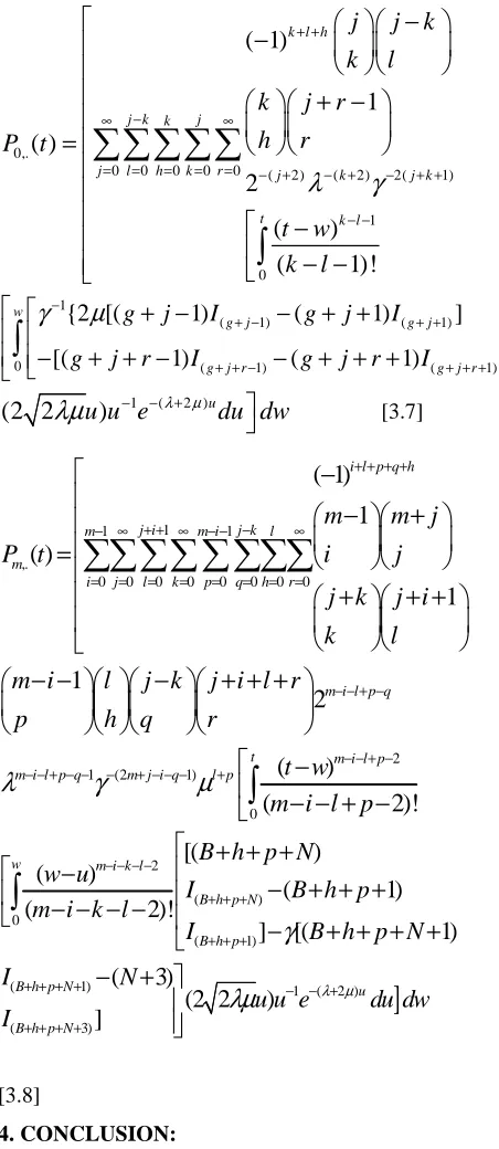
3. NUMBER OF TIMES SYSTEM REACHES ITS CAPACITY IN TIME t

Setting y=1 in [2.18], we have:

1

( ,1; )

1

(1

)

_N

( , )

H x

−

s

=

s





−

λ

−

x P

−₋

x s









[3.1]

1 0,.

[ (

2 )

( )

1

[2 (1)

( ) (

) (

1)]

s s

P s

s

s V

T N

s

T N

λ

−



+



=



−



+

+ +

−





[3.2]

Differentiating [3.2], m times w.r.t. x and dividing

both sides by m! and setting x=0, we have:

2 2

1

,. ₂ ₁

1

(1)[ ( 2 )][ ( 1) ( ) ( ) ( 1) {2 (1) ( ) ( ) ( 1)}] ( )

( 2 ) [2 (1) ( ) ( ) ( 1)]

m

m _m

m

V s s T N

sT N s T N

V T N s T N

P s

s s V T N

s T N

λ λ λ

µ λ λ

λ

− −

−

+

 ₊ ₊ 

 

+ − + −

 

 ₊ _{+ +} ₋ 

= 

+ +

 

+ + −

 

 

[3.4] Expanding the right hand sides of [3.3] and [3.4], we have:

1 0,.

0 0 0 0 0

( 2) ( 2) 2( 1)

1 ( 1) ( 1) 1 ( 1) ( 1)

( 1)

( )

1

2

[

]

[

]

k l h

j k k j

j l h k r

j k j k

g j g j g j r g j r

j

k

P

s

j

k

j

r

l

h

r

R

λ

γ

µγ

γ

+ +

−

∞ ∞

−

= = = = =

− + − + − + +

− − + − − + + − − + + − − + + +



 

−



 

 



=



−

 

+ −







 







 









−







∑∑∑∑∑

[3.5]

1

1 1

,.

0 0 0 0 0 0 0 0

( 1)

1

( )

1

i l p q h

j i j k

m m i l

m

i j l k p q h r

m

j

P

s

i

j

k

j

i

k

l

+ + + +

+ + −

− ∞ ∞ − − ∞

−

= = = = = = = =



−



−

+

















=









+

+ +

























∑∑ ∑ ∑ ∑ ∑∑∑

1

( 2 1) ( 1) ( 1)

2

( ) ( 2 )

m i l p q m i l p q

m j i q l p m i k l m i l p

l j k j i l r

h q r

s s

λ

γ

µ

λ

µ

− − + − − − + − −

− + − − − + − − − − − − − − + +

− + + +

                 

+ +

( ) ( 1) 1 ( 1) ( 3)

[

R

− + +B p N

R

− + +B p

]

γ

−

[

R

− + + +B p N

R

− + + +B p N

]



−







(5)

421 Taking the Inverse Laplace transforms of [3.5] and [3.6], we have

0,.

0 0 0 0 0 ₍ ₂₎ ₍ ₂₎ ₂₍ ₁₎

1

0

( 1)

1

( )

2

(

)

(

1)!

k l h

j k k j

j l h k r _j _k _{j k}

t k l

j

k

l

k

j

r

h

r

P t

t

w

k

l

λ

γ

+ +

−

∞ ∞

= = = = = _{− +} _{− +} ₋ _{+ +}

− −



  

−



−



  



  





 

+ −





 



=



 







−



− −





∑∑∑∑∑

∫

1

( 1) ( 1)

0 ( 1) ( 1)

{2 [(

1)

(

1)

]

[(

1)

(

1)

]

w

g j g j

g j r g j r

g

j

I

g

j

I

g

j

r

I

g

j

r

I

γ

−

µ

+ − + +

+ + − + + +

 

+ −

− + +

 





−

+ + −

− + + +







∫

1 ( 2 )

(2 2

)

u

u u e

λ µ

du dw

λµ

− − +





[3.7]

1

1 1

,.

0 0 0 0 0 0 0 0

1 (2

( 1)

1

( )

1

2

i l p q h

j i j k

m m i l

m

i j l k p q h r

m i l p q

m i l p q m j i q

m

m j

P t

i

j

j k

j i

k

l

m i

l

j k

j i l r

p

h q

r

λ

γ

+ + + +

+ + −

− ∞ ∞ − − ∞

= = = = = = = =

− − + −

− − + − − − + − −



−



−

+

















=









+

+ +

























− −

−

+ + +



 







 







 





∑∑∑∑ ∑∑∑∑

2 1)

0

(

)

(

2)!

t m i l p

l p

t w

m i l p

µ

− − + −

− +



−



− − + −



∫

]

2

( )

0

( 1)

( 1) ₁ ₍ _{2 )}

( 3)

[(

)

(

)

(

1)

(

2)!

]

[(

1)

(

3)

(2 2

)

]

w m i k l

B h p N

B h p

B h p N _u

B h p N

B h p N

w u

I

B h p

m i k l

I

B h p N

I

N

u u e

du dw

I

λ µ

γ

λµ

− − − −

+ + +

+ + + + _{− − +}

+ + + +



+ + +



−



− + + +



− − − −





−

+ + + +



− +







∫

[3.8]

4. CONCLUSION:

In this paper, computing the joint distribution of the number of times M/M/2-(homogeneous servers)/N queueing model reaches its capacity (i.e. finite) in time t. There are several aspects which are a topic for current and future investigations like as computer network, telecommunications, traffic control etc.

REFERENCES

1] Erdelyi, A, W.Magnus, F.Oberhettinger and F.G.Tricomi, (1954), Table of Integral Transform, Vol.1, McGraw-Hill Book Company, New York.

2] Nagarajan, R., Kurose.J, (1997): On defining, computing and guaranteeing quality-of-service in high-speed networks, In: proceeding of INFOCOM’, Vol. 92, pp. 2016-2025.

3] Singh, V.P., (1970), Two-server Markovian queues with balking: Heterogeneous vs. homogeneous Servers, Operations Research, Vol.19, 145-159.

4] Watson, G.N., Sc.D, F.R.S., (1959), A Treatise on the Theory of Bessel Function, 2nd Edition, Cambridge Uni. Press.

5] *Jain, N.K and Garg.(2011), Distribution of the number of times M/M/2/N queuing system reaches its capacity in time t under catastrophic effects”, International journal of computational science and mathematics, Vol. 3, No. 4, 389-400.

6] Jain, N.K and Garg, D, (2011), Distribution of the number of times M/M/2/N queueing system with heterogeneous servers reaches its capacity in time t under catastrophic effects”, International journal of computational and applied mathematics, Vol. 6, No. 2, 169-192. 7] Garg, D, (2013), Distribution of the Number of

Times M/M/2/N Queuing System with Heterogeneous servers reaches its Capacity in Time t subject to Catastrophes and Restorations”, International Journal of Management Research and Development, Vol. 3, No. 4, 31-61,ISSN No: 2248-9398, IF 1.3560. 8] Kleinrock, L. (1975), Queueing systems, Vol. 1,

Wiley, New Yark.

[image:5.595.73.299.130.650.2]