L-band multi-polarization radar
scatterometry over global forests:
modelling, analysis, and applications
Thesis by
Yu Xian Lim
In Partial Fulfillment of the Requirements for the degree of
Doctor of Philosophy
CALIFORNIA INSTITUTE OF TECHNOLOGY Pasadena, California
2020
2019
Yu Xian Lim
ACKNOWLEDGEMENTS
I would like to express my sincere gratitude to my advisor, Dr Jakob J. van Zyl, who introduced me to this field and directly trained me from its basic foundations, and for much guidance, encouragement, and inspiration during the course of this work. A great many important lessons, including those of a technical nature and beyond, were learnt from him.
I would also like to thank the members of my defense and candidacy committees: Professor Ali Hajimiri, Professor P.P. Vaidyanathan, Professor Charles Elachi, and Professor Amnon Yariv.
My gratitude also goes to staff members both at Caltech and JPL: Katey Velazquez, Tanya Owen, Connie Rodriguez, Mariko Burgin.
Acknowledgements to my funding agency, DSO National Laboratories (Singapore) for their generous support.
Much thanks to all my friends who have supported me during my time at Caltech, including members of the Yariv group who welcomed me during my first year.
ABSTRACT
Spaceborne L-band radars have the ability to penetrate vegetation canopies over forested areas, suggesting a potential for regular and frequent global monitoring of both the vegetation state and the subcanopy soil moisture. However, L-band radar’s sensitivity to both vegetation and ground also complicates the relationship between the radar observations and the ecological and geophysical parameters. Accurate yet parsimonious forward models of the radar backscatter are valuable to building an understanding of these relationships. In the first part of this thesis, a model of L-band multi-polarization radar backscatter from forests,
TABLE OF CONTENTS
Acknowledgements iii
Abstract iv
Table of Contents vi
Chapter 1: Introduction 1
1.1 Background and overview 1
1.2 Radar scattering geometry and scattering matrix 5
1.3 Radar cross-sections and distributed targets 9
1.4 Scatterer covariance matrix 10
1.5 Optical theorem 11
Chapter 2: Modelling of L-band Radar Backscatter From Forests 13
2.1 Overview of modelling approach 13
2.2 Backscatter from crown canopy layer only 15
2.3 Direct backscatter from the ground 22
2.4 Double-reflections off the ground and crown canopy layer 25
2.5 Trunk-ground double reflections 29
2.6 Cylinder relative permittivity εv 31
2.7 Distribution of cylinder radius and length in the crown canopy layer 32
2.8 Distribution of cylinders in the trunk layer 40
Chapter 3: Application of L-band Radar Backscatter Model to Aquarius Data
over Global Forests 46
3.1 Chapter overview 46
3.2 Input datasets 47
3.3 Evergreen needleleaf forests (IGBP class 1) 53
3.4 Evergreen broadleaf forests (IGBP class 2) 70
3.5 Deciduous needleleaf forests (IGBP class 3) 78
3.6 Deciduous broadleaf forests (IGBP class 4) 85
3.7 Mixed forests (IGBP class 5) 91
3.8 Frozen vs. unfrozen conditions 100
3.9 Microwave vegetation optical depth 104
Chapter 4: Diurnal effects on L-band Radar Backscatter over Global Forests
Using SMAP 107
4.1 Chapter introduction and overview 107
4.2 SMAP dataset 108
4.3 Beam azimuth effects 111
4.4 Diurnal effects 114
Chapter 5: Algorithms for Soil Moisture Retrieval from Forests Using L-band
Scatterometry 127
5.1 Chapter overview 127
5.2 Proposed soil moisture retrieval algorithms 127
5.4 Conclusion 147
Bibliography 149
Appendix A: Bistatic Scattering from a Dielectric Cylinder 162
Appendix B: Multiple Scattering Correction Factor 166
C h a p t e r 1
INTRODUCTION
1.1 Background and overview
The ability to model and predict feedbacks in a changing climate requires many inputs, including knowledge of where, when, and how much carbon, water, and energy are stored and exchanged between the land surface and the atmosphere. Many of these interactions take place in forests, which are major carbon sinks, and contain a majority of global plant biomass [1]. However, there is significant uncertainty in the knowledge of some of these variables and their fluxes. Importantly, soil moisture, a key element in evapotranspiration, climate state, weather and landslide prediction, and flood and drought monitoring [2], is poorly measured in forests [3, 4]. There is also significant uncertainty in the total biomass carbon stock of forests, the rate at which it is changing due to deforestation and regrowth, and their associated spatial distributions [5, 6, 7].
Spaceborne remote sensing offers a good platform to study such key elements pertinent to the understanding of our climate and environment on a global scale. In particular, microwave remote sensing enables timely monitoring without interruption by cloud cover and can measure geophysical parameters that are complementary to the visible-infrared part of the electromagnetic spectrum. Over forested land areas, long wavelength microwaves, e.g. at L-band, can penetrate the vegetation canopy and offer sensitivity to both the vegetation as well as to moisture in the ground under the canopy [8, 9], holding promise as a tool for learning about changes in their state and related processes if multiple and frequent observations over time are available.
synthetic aperture techniques allow finer spatial resolutions to be tailored according to specific application requirements.
Amongst the spaceborne L-band radar missions that have flown, two stand out in terms of temporal coverage and polarization information: Aquarius and SMAP (Soil Moisture Active Passive). Aquarius has a 7-day repeat orbit, while SMAP has global coverage every 2-3 days. They also offer the advantage of full multi-polarization measurements, sending and receiving in both horizontal and vertical polarizations. Polarization information has long been recognized to be useful in helping to distinguish different scattering mechanisms involving the vegetation and ground [10, 11, 12, 13]. This is important because the sensitivity of L-band radar to both vegetation and ground is a double-edged sword that complicates the retrieval of their ecological and geophysical parameters from the radar observations.
Having motivated the study of forested areas and identified the opportunity provided by the L-band multi-polarization radars of Aquarius and SMAP, in this thesis we study L-band radar backscatter from forests to better understand its spatial and temporal relationships and sensitivities to the underlying physical conditions, with the aid of polarization information. It is worthwhile to mention that Aquarius was not a mission that was originally intended for observations over land, but instead for the measurement of ocean salinity. SMAP, though focused on soil moisture, was not primarily targeted at forested areas, due in part to limitations in understanding the relationships between the L-band measurements and subcanopy soil moisture in the presence of significant intervening vegetation. On the other hand, there have been previous studies dedicated to studying L-band radar backscatter from forests, but these have been over specific, localized forest stands in the context of airborne synthetic aperture radar (SAR) experiments [9, 14, 15, 16]. There is thus significant potential in exploiting the Aquarius and SMAP radar measurements over forests for analysis and interpretations at the regional to global scale.
dielectric constants, and ground conditions were made concurrently with airborne SAR measurements. These efforts helped to validate many of the concepts and approaches used in the models. Extending the modelling effort to a global scale, Kim et al. [22] have developed physical models of L-band radar backscatter for application to soil moisture retrieval. In particular, their model for forests was based on work by Tabatabaeenejad et al. [9] and Burgin et al. [21], which required a detailed and complete characterization of the geometry of vegetation structures as input. To reduce the number of free input parameters required, each forest land cover class was modelled with representative species, and species-specific allometric relations were applied to relate all vegetation parameter to a single free input parameter – vegetation water content (VWC). In-situ samples from field measurements were also used as training data to tune some geometric parameters within the model. Two other input parameters, soil surface root mean square (RMS) height and soil dielectric constant, describe the ground. Such parsimony was essential for model inversion and parameter estimation from limited data – only three measurement channels (HH, HV, VV polarization) from the radar of the Soil Moisture Active Passive (SMAP) mission.
providing accurate agreement between the model and data, especially when the dynamic range in the radar backscatter from forests is only several decibels. Further modelling details are described in Chapter 2.
Equipped with our forward model which relates radar backscatter to input parameters from the forest and ground, in Chapter 3 we apply it to the analysis of global forest L-band multi-polarization backscatter data from the Aquarius scatterometer. We show that our model appears to be consistent with the data overall, and interpret spatial and temporal variations in the radar backscatter in terms of ground and vegetation factors. Neither ground nor vegetation factors alone suffices to explain the spatial variance within the same land cover class. For temporal variations during unfrozen periods, soil moisture may be a primary factor at timescales of one week to several months. Vegetation changes remain a non-negligible factor, and for larger incidence angles over deciduous needleleaf forests may even become the primary factor at longer timescales (months). Differences in L-band radar due to freeze/thaw states, branch orientation, and flooding were also partially verified quantitatively
with our model.
In Chapter 4, we analyze diurnal variations in L-band multi-polarization backscatter from forests using SMAP data. Transpiration and related plant processes follow a diurnal cycle and there is potential for monitoring vegetation water status using radar [23, 24, 25, 26, 27]. We find that the co-polarized L-band radar backscatter observed in late spring-summer over the northern boreal forests is higher at 6PM than 6AM, which is not what one might expect based on previous studies. Based on our modelling, increased canopy extinction at 6AM is a possible cause, but this is unproven and its true underlying physical cause is undetermined. Aside from the diurnal variations, we also report the observation of significant differences in backscatter due to beam azimuthal angle, possibly associated with plant phototropism.
radar backscatter and subcanopy soil moisture, under certain conditions. Based on this linear relationship, we propose some algorithms for soil moisture retrieval from forests using L-band radar. Preliminary evaluations suggest improved performance over existing algorithms.
The subsequent sections in this chapter will briefly review some preliminary foundations that are essential for subsequent chapters. The content can be found in most radar textbooks, though notations and conventions vary; here we largely follow the notations and conventions adopted by Ulaby and Long [28]. In Section 1.2, we establish the scattering geometry and coordinate system, and define the 2x2 scattering matrix. Section 1.3 reviews the radar cross-section for a point target and a distributed target. Section 1.4 covers the scatterer covariance matrix, and Section 1.5 the optical theorem. We shall not derive these concepts from first principles; rather, we merely provide the definitions to set the stage for their use in the rest of the thesis.
1.2 Radar scattering geometry and scattering matrix
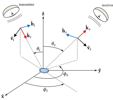
Here we establish the notations, geometries, and coordinate systems to be used. Consider a single point scatterer, or target, located at the origin with the scattering geometry as in Figure 1.1. The incident direction is 𝐤̂ 𝑖, the scattered direction is 𝐤̂ 𝑠, with
𝐤̂𝑖 = sin 𝜃𝑖cos 𝜙𝑖𝐱̂ + sin 𝜃𝑖sin 𝜙𝑖𝐲̂ − cos 𝜃𝑖𝐳̂ (1. 1)
𝐤
̂ 𝑠 = sin 𝜃𝑠cos 𝜙𝑠𝐱̂ + sin 𝜃𝑠sin 𝜙𝑠𝐲̂ + cos 𝜃𝑠𝐳̂ (1. 2)
𝐡
̂ 𝑖 = 𝐳̂ × 𝐤̂ 𝑖
|𝐳̂ × 𝐤̂ 𝑖|
, 𝐯̂𝑖 = 𝐡̂𝑖× 𝐤̂ 𝑖 , 𝐡̂ 𝑠 = 𝐳̂ × 𝐤̂ 𝑠 |𝒛̂ × 𝐤̂ 𝑠|
, 𝐯̂𝑠 = 𝐡̂ 𝑠× 𝐤̂ 𝑠 . (1. 3)
Figure 1.1. Geometry for the FSA (forward-scattering alignment) convention.
Let
𝐄𝑖 = (𝐸ℎ𝑖𝐡̂ 𝑖+ 𝐸𝑣𝑖𝐯̂𝑖) exp[𝑖𝑘𝐤̂ 𝑖∙ 𝐫 − 𝜔𝑡] (1. 4)
be an incident plane wave propagating in the 𝐤̂ 𝑖 direction, where 𝑘 = 2𝜋/𝜆 is the wavenumber, and 𝜔 = 2𝜋𝑓is the angular frequency. 𝐡̂𝒊 and 𝐯̂𝒊 are mutually orthogonal unit vectors also orthogonal to 𝐤̂ 𝑖, as defined in (1.3) and Figure 1.1. Likewise, let
𝐄𝑠 = (𝐸ℎ𝑠𝐡̂ 𝑠+ 𝐸𝑣𝑠𝐯̂𝑠) exp[𝑖𝑘𝐤̂ 𝑠∙ 𝐫 − 𝜔𝑡] (1. 5)
be the scattered field (in the far-field) in the 𝐤̂ 𝑠direction, with 𝐡̂ 𝑠 and 𝐯̂𝑠 mutually orthogonal unit vectors also orthogonal to the scattered direction 𝐤̂ 𝑠. The terms “h-polarized” and
“v-𝐡
̂
𝑖𝐯̂
𝑖𝐡
̂
𝑠𝐯̂
𝑠𝐤
̂
𝑠𝐤
̂
𝑖𝜃
𝑖𝜃
𝑠𝜙
𝑖𝜙
𝑠𝐳̂
𝐱̂
𝐲̂
polarized” will be used frequently with regards to the incident or scattered fields. The relation between the scattered and incident fields can be conveniently written in matrix form
[𝐸ℎ
is the (dimensionless) scattering matrix for the single point scatterer (some other authors in the literature prefer to put the factor of 1/𝑘 within the matrix rather than outside, such that the scattering matrix has dimensions of length). The four entries of this 2x2 matrix are the scattering amplitudes for the respective polarizations. Note that the scattering matrix is dependent on the choice of polarization basis vectors 𝐡̂ 𝑖, 𝐯̂𝑖, 𝐡̂𝑠, 𝐯̂𝑠. These equations are written for linearly-polarized incident waves, but arbitrary elliptical polarizations can be readily accommodated with suitable complex phases.
Figure 1.1, and equations (1.1) to (1.3) represent a common choice of coordinate basis, the FSA convention. Another choice of coordinate basis is the “BSA (backscatter alignment) convention”, or so-called antenna coordinates [28]:
𝐤
Figure 1.2. Geometry for the BSA (backscatter alignment) convention.
Throughout this thesis, both conventions are used. The BSA convention is more convenient when in the backscatter (monostatic) case, because then 𝐤̂ 𝑖 = 𝐤̂ 𝑠, while FSA is more convenient in the bistatic case when the incident and scattered directions are arbitrary. The scattering matrices in either convention can be converted to the other convention simply:
[𝐒(𝜃𝑖, 𝜙𝑖, 𝜃𝑠, 𝜙𝑠)]𝐵𝑆𝐴 = [−1 0
0 1] [𝐒(𝜃𝑖, 𝜙𝑖, 𝜃𝑠, 𝜙𝑠)]𝐹𝑆𝐴 . (1. 11)
Whenever the scattering matrix is used, the convention used (BSA or FSA) will not be labelled as a subscript, but will instead be clarified in the text. Note that the quantities |𝑆ℎℎ|2,
|𝑆ℎ𝑣|2, |𝑆𝑣ℎ|2, |𝑆𝑣𝑣|2 are the same in either convention.
𝐡
̂
𝑖𝐯̂
𝑖𝐡
̂
𝑠𝐯̂
𝑠𝐤
̂
𝑠𝐤
̂
𝑖𝜃
𝑖𝜃
𝑠𝜙
𝑖𝜙
𝑠𝐳̂
𝐱̂
𝐲̂
1.3 Radar cross-sections and distributed targets
Suppose the incident radar is h-polarized and illuminates the point target with a power density of 𝒮ℎ𝑖, with units of W/m2 (power per unit area, where the area is normal to the propagation direction). The power 𝑑𝑃𝑣𝑠 scattered into the far-field into an infinitesimal solid angle 𝑑Ω in the direction 𝐤̂ 𝑠, in the v-polarization, is then
𝑑𝑃𝑣𝑠 =
|𝑆𝑣ℎ|2
𝑘2 𝒮ℎ𝑖𝑑Ω . (1. 12)
Analogous equations hold for other combinations of incident and scattered polarizations. The radar scattering cross-section, 𝜎𝑣ℎ, also called the radar cross-section or RCS, is by
So far all discussion has been concerning a single point target. In cases of a distributed target or collection of scatterers extending over an area, such as the ground, the normalized radar cross-section, 𝜎𝑣ℎ0 , (NRCS, also referred to as differential scattering coefficient) is defined as the radar cross-section per unit horizontal ground area [28]
𝜎𝑣ℎ0 = 〈𝜎𝑣ℎ〉
𝐴 (1. 14)
where A is a unit horizontal ground area, and 〈𝜎𝑣ℎ〉 is the average value of 𝜎𝑣ℎ over that area. 𝜎𝑣ℎ0 is dimensionless and as usual, analogous equations hold for other combinations of incident and scattered polarizations. For a thin horizontal layer of randomly distributed identical small scatterers, with an average scatterer number density of 𝑛 (i.e. 𝑛 has units of m-3) and layer thickness of Δ𝑧,
𝜎𝑣ℎ0 = 4𝜋𝑛Δ𝑧
If the scatterers are not identical, equation (1.15) still holds with the angular brackets being interpreted as also averaging over the distribution of scatterers.
As a shorthand notation, instead of 𝜎ℎℎ0 , 𝜎𝑣ℎ0 , 𝜎ℎ𝑣0 , 𝜎𝑣𝑣0 , often HH, VH, HV, VV are used
Due to the large dynamic range of possible normalized radar cross-sections and abundance of factors that combine multiplicatively, decibels (dB) are often used instead of linear units. They can be readily converted via
(𝑞𝑢𝑎𝑛𝑡𝑖𝑡𝑦 𝑖𝑛 𝑑𝑒𝑐𝑖𝑏𝑒𝑙𝑠)dB = 10 log10(𝑞𝑢𝑎𝑛𝑡𝑖𝑡𝑦 𝑖𝑛 𝑙𝑖𝑛𝑒𝑎𝑟 𝑢𝑛𝑖𝑡𝑠) . (1. 17)
1.4 Scatterer covariance matrix
[𝐂] = [
The diagonal entries of the covariance matrix are proportional to the respective normalized radar cross-sections, but the covariance matrix contains additional information about the relative phase between different polarizations in the off-diagonal entries.
1.5 Optical theorem
The optical theorem (see e.g. [32], [30], [33]), also known as the forward scattering theorem, relates the extinction to the forward scattering amplitude rather generally for scattering phenomena. Newton [34] traces its more-than-a-century old history. To state it for our case, the extinction cross-section for a single scatterer is, for h-polarized and v-polarized incident radar beams respectively,
where the forward scattering amplitudes are in FSA.
For instance, the intensity or power of a h-polarized incident beam propagating in the 𝐱̂
direction through a cloud of identical scatterers with number density 𝑛 (𝑛 has units of m−3), decays as
𝐼ℎ(𝑥) = 𝐼ℎ(𝑥 = 0) exp [−𝑛𝜎𝑒𝑥𝑡,ℎ(𝜃𝑖 =
𝜋
2, 𝜙𝑖= 0) 𝑥] (1. 21)
and likewise for v-polarization. If the scatterers are not identical, we can assign an average cross-section over the distribution of scatterers such that we retain the expression
𝐼ℎ(𝑥) = 𝐼ℎ(𝑥 = 0) exp [−𝑛 〈𝜎𝑒𝑥𝑡,ℎ(𝜃𝑖 =𝜋
2, 𝜙𝑖 = 0)〉 𝑥] (1. 22)
The electric field amplitude is proportional to the square root of the intensity; for ease of future notation, we introduce the corresponding average-per-scatterer extinction cross-section for the field
〈𝜅ℎ(𝜃𝑖, 𝜙𝑖)〉 =
1
2〈𝜎𝑒𝑥𝑡,ℎ(𝜃𝑖, 𝜙𝑖)〉 = 2𝜋
𝑘2〈Imag[𝑆ℎℎ(𝜃𝑖, 𝜙𝑖, 𝜃𝑠 = 𝜋 − 𝜃𝑖, 𝜙𝑠 = 𝜙𝑖)]〉 (1. 23)
C h a p t e r 2
MODELLING OF L-BAND RADAR BACKSCATTER FROM FORESTS
2.1 Overview of modelling approach
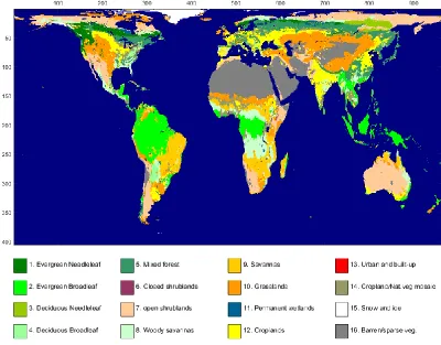
In this chapter, a model to simulate the L-band radar backscatter from forests will be presented. As mentioned in the introduction, this model is intended primarily for regional to global spatial scales. Globally, there is a wide variation in the density and types of vegetation cover over land. We shall use the land cover classification adopted by the International Geosphere-Biosphere Program (IGBP) [35]. (A map of global land cover in the IGBP classification scheme can be found in Figure 3.5.) Classes 1-5 correspond to forests classes. Numerous different species of trees and inhomogeneous distributions are expected within the radar footprint. Instead of attempting to describe them all in detail, broad simplifications are made here. The forest is modelled as a homogenous layer of randomly oriented dielectric cylinders corresponding to crown canopy branches (leaves and structures of other morphologies are neglected), and a lower homogeneous layer of preferentially vertically oriented dielectric cylinders corresponding to tree trunks. Four separate terms contributing to the radar backscatter, corresponding to different scattering mechanisms, are considered. They are: 1. Backscatter from the crown canopy layer only; 2. direct backscatter from the ground; 3. double-reflections off the ground and canopy layer; 4. double-reflections off the ground and tree trunks. This is depicted schematically in Figure 2.1. These terms are then added incoherently together to give the total backscatter. For each polarization, the radar cross section per unit ground area is represented as:
𝜎0 = 𝜎
𝑐𝑛0 + 𝜎𝑔𝑛𝑑,𝑑𝑖𝑟𝑒𝑐𝑡0 + 𝜎𝑐𝑛−𝑔𝑛𝑑,𝑑𝑏0 + 𝜎𝑡𝑟𝑘−𝑔𝑛𝑑,𝑑𝑏0 . (2. 1)
Figure 2.1. Model of L-band radar backscatter from natural vegetation, as the incoherent sum of four separate terms corresponding to different scattering mechanisms.
The modelling approach adopted here largely follows that taken by Durden et al. [14] and Burgin et al. [21], with some important novel developments. This approach required a detailed specification of the sizes and geometries of all the cylinders involved, which typically involved intensive measurements of several sample trees at specific field study sites. In those experiments, such a complete characterization was ideal for direct validation of the modelling approach against concurrent SAR measurements. However, because we intend to apply our model to many different parts of the globe, usually without detailed knowledge of the required physical and geometric parameters, we try to keep the model with as few free input parameters as possible. The importance of this parsimony was also emphasized by Tabatabaeenejad et al. [9] and Kim et al. [22], bearing in mind that in application, model inversion and parameter estimation are expected to be performed from limited measurement channels – just the three polarization channels HH, HV, VV in the case of the Aquarius and SMAP radars. A novel development in our approach is to go beyond the
species-specific allometry in Tabatabaeenejad et al. [9] and Kim et al. [22], and apply a general plant allometry model, which thus also mitigates the need for much intensive field data for training and/or over-tuning towards specific sites and samples; in both a literal and figurative sense, to not lose the forest for the trees. This will be further explained and elaborated upon in Section 2.7 and Section 2.8.
The retained free input parameters to our model are: the total canopy branch volume per unit ground area, 𝑉𝑏,𝑡𝑜𝑡, in units of m3/m2; the relative permittivity of the vegetation, 𝜀𝑣; the relative permittivity of the ground, 𝜀𝑔; and the RMS height of the roughness of the ground surface, ℎ, in units of m. There are additional parameters pertaining to the orientation distribution of the cylinders that can be chosen, but these will not be freely varying.
Another important novel departure we make from Durden et al. [14] and Burgin et al. [21] is that, for the backscatter term from the canopy layer only, while we still employ a single-scattering approximation for computational simplicity, we make a correction for multiple scattering effects within the canopy; this correction is particularly significant for forests.
Details for computing each of the four modelled terms are elaborated in the sections below.
2.2 Backscatter from crown canopy layer only
√𝜀eff,ℎ−𝑝𝑜𝑙 = 1 +
where 𝑛𝑐𝑛 has units of inverse volume and is the number density of scatterers (i.e. cylinders) in the canopy layer, and 𝑘 = 2𝜋/𝜆 is the wavenumber in air. Here the forward scattering amplitudes are in the FSA convention (see Section 0), and angular brackets denote averaging over the cylinder distribution. The cylinders “see” the incident radar wave modified correspondingly by an extinction and phase delay, and make a single scattering back to the radar receiver. (Multiple-scatterings are accounted for by a correction later.) Cylinders deeper in the layer make less contribution to the total backscatter due to extinction from higher parts. The electric field decays exponentially with depth with an extinction coefficient (for h- and v-polarizations respectively) related to the imaginary part of the forward
consistent with the optical theorem (Section 2.4); the extinction coefficient for the intensity is twice that for the field. The phase delay can be found from the real part of the forward scattering amplitude, and needs to be considered if it is polarization-dependent and phase differences between polarizations are required. Otherwise if only normalized radar cross-sections are required, this phase can be ignored.
Scattering matrices for both the forward and backward scattering from the cylinders are required. For a single cylinder with relative permittivity 𝜀𝑣, radius 𝑟, length 𝐿, and orientated with cylinder axis direction (𝜃𝑐, 𝜙𝑐), the 2x2 dimensionless bistatic scattering matrix
and scattering angles (𝜃𝑖, 𝜙𝑖) and (𝜃𝑠, 𝜙𝑠) may follow either the FSA or BSA conventions (see Section 1.2);recall that the 2x2 scattering matrix in the BSA and FSA conventions only differ by a change of sign in 𝑆ℎℎ and 𝑆ℎ𝑣 (see equation (1.11)). The relative permittivity within each cylinder is assumed to be homogeneous, and all cylinders in the vegetation layer are assumed to have the same relative permittivity, so we do not display the dependence of
[𝐒] on 𝜀𝑣.
We can now discuss in further detail the averaging operations over cylinder distribution that have been referred to with angular brackets. Let 𝑝(𝜃𝑐, 𝜙𝑐, 𝑟, 𝐿) be the density function of the cylinder size and orientation distribution, satisfying the normalization
∫ ∫ 𝑝(𝜃𝑐, 𝜙𝑐, 𝑟, 𝐿) sin 𝜃𝑐𝑑𝜃𝑐𝑑𝜙𝑐𝑑𝑟𝑑𝐿
𝜃𝑐,𝜙𝑐 𝑟,𝐿
= 1 . (2. 4)
Averaging over the cylinder distribution thus means, for instance,
〈[𝐒(𝜃𝑖, 𝜙𝑖, 𝜃𝑠, 𝜙𝑠)]〉 = ∫ ∫ [𝐒(𝜃𝑖, 𝜙𝑖, 𝜃𝑠, 𝜙𝑠, 𝜃𝑐, 𝜙𝑐, 𝑟, 𝐿)]𝑝(𝜃𝑐, 𝜙𝑐, 𝑟, 𝐿) 𝜃𝑐,𝜙𝑐
𝑟,𝐿
sin 𝜃𝑐𝑑𝜃𝑐𝑑𝜙𝑐𝑑𝑟𝑑𝐿 . (2. 5)
For simplicity, the size and orientation of the cylinders are modelled as being independent, i.e. 𝑝(𝜃𝑐, 𝜙𝑐, 𝑟, 𝐿) can be factorized accordingly. Integrals over the cylinder orientations
scattering calculations, an angular discretization of 0.35𝜆/𝜋𝐿 was used. This angular discretization is chosen in view of the width of the sinc function in equation (A. 1) in Appendix A. If 0.35𝜆/𝜋𝐿 is greater than 5, the angular discretization is set at 5 instead.
calculation, the relevant parameter is instead the average number of cylinders per unit ground area, not 𝑛𝑐𝑛 and (𝑍2− 𝑍1) separately.
Thus far, the validity of the single-scattering approximation has been implicitly relied upon.
HH𝑐𝑛,𝑠𝑠, VV𝑐𝑛,𝑠𝑠 and HV𝑐𝑛,𝑠𝑠 shall be referred to as the “single-scattering solutions” for the backscatter from the canopy layer. When the vegetation gets thick, multiple scattering paths may become important. We attempt to take this into account by applying a polarization-dependent multiple scattering correction factor, denoted ℱ, such that our full solution for the backscatter from the canopy layer that includes multiple scattering effects is
HH𝑐𝑛 = ℱHH(𝜏𝑐𝑛(𝜃𝑖), 𝜃𝑖, 𝜀𝑣)HH𝑐𝑛,𝑠𝑠 (2. 8a)
VV𝑐𝑛 = ℱVV(𝜏𝑐𝑛(𝜃𝑖), 𝜃𝑖, 𝜀𝑣)VV𝑐𝑛,𝑠𝑠 (2.8b)
HV𝑐𝑛= ℱHV(𝜏𝑐𝑛(𝜃𝑖), 𝜃𝑖, 𝜀𝑣)HV𝑐𝑛,𝑠𝑠 . (2.8c)
The multiple scattering correction factor ℱ depends on the incident angle 𝜃𝑖, the cylinder relative permittivity 𝜀𝑣, and the simplified average optical thickness of the canopy layer,
𝜏𝑐𝑛(𝜃𝑖), where
𝜏𝑐𝑛(𝜃𝑖) =
𝑛𝑐𝑛(〈𝜅ℎ,𝑐𝑛(𝜃𝑖)〉 + 〈𝜅𝑣,𝑐𝑛(𝜃𝑖)〉)(𝑍2− 𝑍1) cos 𝜃𝑖
. (2. 9)
For compactness, 𝜏𝑐𝑛 instead of 𝜏𝑐𝑛(𝜃𝑖) may be written subsequently, with implied dependence on the incidence angle 𝜃𝑖.
To estimate ℱHH and ℱVV, the method of radiative transfer [40] was used to calculate the backscatter without making the single-scattering assumption. The radiative transfer calculation was performed for several values of 𝜏𝑐𝑛, 𝜃𝑖, and 𝜀𝑣, with a uniformly random cylinder orientation distribution for (𝜃𝑐, 𝜙𝑐), and a specific distribution over cylinder radii 𝑟 and lengths 𝐿; details of this radiative transfer calculation are provided in Appendix B. A further correction is made to account for coherent backscatter enhancement not modelled by the radiative transfer equations. Interpolation is used to find ℱ for intermediate values of
cross-polarization and co-cross-polarization returns for double scattering from the same cylinder distribution. More details are provided in Appendix B. Note that we only compute these multiple-scattering correction factors once for a fixed cylinder distribution, and apply these correction factors even for other cylinder distributions. The reason for this is that the multiple scattering computations are far more demanding than the single-scattering calculation. The multiple scattering correction factor was checked at a few values of 𝜏𝑐𝑛, 𝜃𝑖, 𝜀𝑣 to be similar to if a cosine-squared cylinder orientation distribution was used instead of a uniformly random orientation distribution, partially justifying this simplification.
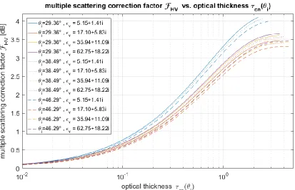
The multiple scattering correction factor ℱ(𝜏𝑐𝑛, 𝜃𝑖, 𝜀𝑣) is plotted below in Figure 2.2 to Figure 2.4 as a function of the optical thickness 𝜏𝑐𝑛(𝜃𝑖) for several computed values of 𝜃𝑖
Figure 2.2. Estimated multiple-scattering correction factor ℱHH(𝜏𝑐𝑛(𝜃𝑖), 𝜃𝑖, 𝜀𝑣) as a function of
optical thickness 𝜏𝑐𝑛(𝜃𝑖), for several values of 𝜃𝑖 and 𝜀𝑣 .
Figure 2.3. Estimated multiple-scattering correction factor ℱVV(𝜏𝑐𝑛(𝜃𝑖), 𝜃𝑖, 𝜀𝑣) as a function of
Figure 2.4. Estimated multiple-scattering correction factor ℱHV(𝜏𝑐𝑛(𝜃𝑖), 𝜃𝑖, 𝜀𝑣) as a function of
optical thickness 𝜏𝑐𝑛(𝜃𝑖), for several values of 𝜃𝑖 and 𝜀𝑣 .
2.3 Direct backscatter from the ground
This section describes the computation of the second term contributing to the overall radar backscatter, 〈𝜎𝑝𝑜𝑙0 〉𝑔𝑛𝑑,𝑑𝑖𝑟𝑒𝑐𝑡 for 𝑝𝑜𝑙 = ℎℎ, 𝑣𝑣, ℎ𝑣. For direct backscatter from the ground, we use the simplified IEM model by Fung and Chen [41]. The ground is modelled as a flat, horizontal, slightly rough surface with dielectric constant 𝜀𝑔. The roughness is assumed to be a Gaussian process with RMS height ℎ and exponential correlation with correlation length
𝜁. 𝜃𝑖 is the radar incidence angle and 𝑘 = 2𝜋/𝜆 is the wavenumber as usual. The normalized backscatter radar cross-section is then given in terms of these parameters by [41]:
where
𝐼ℎℎ𝑛 = (2𝑛exp[−𝑘2ℎ2cos2𝜃
𝑖] 𝑓ℎℎ+ 𝒢ℎℎ)(𝑘ℎ cos 𝜃𝑖)𝑛 (2. 11a)
𝐼𝑣𝑣𝑛 = (2𝑛exp[−𝑘2ℎ2cos2𝜃
𝑖] 𝑓𝑣𝑣+ 𝒢𝑣𝑣)(𝑘ℎ cos 𝜃𝑖)𝑛 (2.11b)
For an isotropic correlation function, the dependence is only on the magnitude of the distance between two points. The surface spectrum (by the Wiener-Khinchin theorem) of an exponential correlation raised to the n-th power is, in polar coordinates,
𝐹𝑡 =
In our numerical computation, we use only the first twenty terms of the infinite series, as a trade-off between computational accuracy and speed.
Fung and Chen [41] also provide expressions for the polarized backscatter. This cross-polarized backscatter term from the ground is neglected here because it is small compared to the cross-polarized backscatter from the vegetation layer, i.e. let
HV𝑔𝑛𝑑,𝑑𝑖𝑟𝑒𝑐𝑡= 0. (2. 13)
Strictly speaking, this approximation is only valid when the ground surface is reasonably flat, but because forested areas have strong cross-polarized backscatter from the vegetation, this approximation is good except in very extreme cases e.g. mountainous areas. When applying our model in subsequent chapters, we shall exclude areas with high terrain slope.
the relationship between soil moisture and 𝜀𝑔 is provided in Appendix C. We shall not need to explicitly use this relationship until Chapter 5, where it will be discussed further; until then, it suffices for us to work in terms of 𝜀𝑔.
2.4 Double-reflections off the ground and crown canopy layer
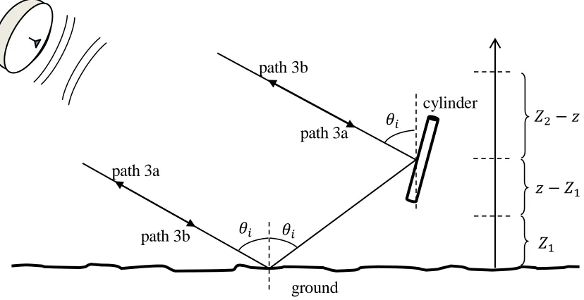
This section describes the computation of the third term contributing to the overall radar backscatter, 〈𝜎𝑝𝑜𝑙0 〉𝑣𝑛−𝑔𝑛𝑑,𝑑𝑏 for = ℎℎ, 𝑣𝑣, ℎ𝑣. Figure 2.5 is a schematic of the double-reflection off the ground and a cylinder in the upper crown canopy layer. The cylinder is at a height 𝑧 above the ground, 𝑍1 ≤ 𝑧 ≤ 𝑍2. 𝑍1 is the total height of the lower trunk layer, and
𝑍2− 𝑍1 is the total height of the upper crown canopy layer. Note that there are two exactly opposite pathways that add coherently. Let path 3a be the path that scatters off the cylinder first, and then the ground, before returning to the radar antenna. Let path 3b be the opposite path that scatters off the ground first, and then the cylinder, before returning to the radar antenna. To find the double-bounce backscatter, the bistatic scattering off the cylinder, bistatic scattering off the ground, extinction through the upper crown canopy layer, and extinction through the lower trunk layer are required.
Figure 2.5. Double reflections off the ground and a cylinder in the upper vegetation volume layer are a coherent sum of two opposite pathways, labelled 3a and 3b.
𝜃𝑖
𝜃𝑖 𝜃𝑖 path 3b
path 3a
path 3b path 3a
cylinder
ground
𝑍1
𝑧 − 𝑍1
Let
[𝐒𝑐𝑦𝑙,3𝑎] = [𝑆ℎℎ 𝑆ℎ𝑣
𝑆𝑣ℎ 𝑆𝑣𝑣]𝑐𝑦𝑙,3𝑎 (2. 14)
be the 2x2 dimensionless bistatic scattering matrix off the cylinder for incidence from direction (𝜃𝑖, 𝜙𝑖) and scattering into direction (𝜃𝑠 = 𝜋 − 𝜃𝑖, 𝜙𝑠 = 𝜙𝑖+ 𝜋), and [𝐆] be the 2x2 dimensionless bistatic scattering matrix off the ground for incidence from direction
(𝜃𝑖, 𝜙𝑖) and scattering into direction (𝜃𝑠 = 𝜃𝑖, 𝜙𝑠 = 𝜙𝑖), both written in their local BSA coordinates. As before, [𝐒𝑐𝑦𝑙,3𝑎] is provided by the expressions in Appendix A. For [𝐆] , the Fresnel reflection coefficients are used, with a correction for surface roughness found from a physical optics approximation (also often called the Kirchhoff approximation) [44, 14]
[𝐆] = [𝐺ℎℎ 0
𝑖) is the roughness correction factor.
The extinction cross-sections (normalized to one cylinder) through the upper crown canopy layer were 〈𝜅ℎ,𝑐𝑛〉 and 〈𝜅𝑣,𝑐𝑛〉 for h-polarized and v-polarized electric field respectively. Likewise, let 〈𝜅ℎ,𝑡𝑟𝑘〉 and 〈𝜅𝑣,𝑡𝑟𝑘〉 be the extinction cross-sections (normalized to one cylinder) through the lower trunk layer for h-polarized and v-polarized electric field, with units of area, and 𝑛𝑡𝑟𝑘 be the average number density of cylinders in the trunk layer, with units of inverse volume.
𝛼ℎ,𝑡𝑟𝑘(𝑍1) = exp [−𝑛𝑡𝑟𝑘〈𝜅ℎ,𝑡𝑟𝑘〉𝑍1
For convenience in multiplication with 2x2 scattering matrices, let
[𝛂𝑡𝑟𝑘(𝑍1)] = [
𝛼ℎ,𝑡𝑟𝑘(𝑍1) 0 0 𝛼𝑣,𝑡𝑟𝑘(𝑍1)
] . (2. 18)
Likewise, for the upper crown canopy layer, the one-way extinction of the electric field through the part of the upper crown canopy layer above the cylinder, written as a 2x2 matrix, is
Similarly, the one-way extinction of the electric field through the part of the upper crown canopy layer below the cylinder is [𝛂𝑐𝑛(𝑧 − 𝑍1)], and the total one-way extinction of the electric field through the upper crown canopy layer is [𝛂𝑐𝑛(𝑍2− 𝑍1)].
We can now write the overall 2x2 scattering matrix for path 3a as
[𝑆ℎℎ 𝑆ℎ𝑣
𝑆𝑣ℎ 𝑆𝑣𝑣]3𝑎= [𝛂𝑐𝑛(𝑍2− 𝑍1)][𝛂𝑡𝑟𝑘(𝑍1)][𝐆] [−1 00 1]
× [𝛂𝑡𝑟𝑘(𝑍1)][𝛂𝑐𝑛(𝑧 − 𝑍1)][𝐒𝑐𝑦𝑙,3𝑎] [𝛂𝑐𝑛(𝑍2− 𝑧)] (2. 20)
where the factor of [−1 0
0 1] accounts for the direction of the axes in the BSA convention.
[𝑆ℎℎ 𝑆ℎ𝑣
Paths 3a and 3b combine coherently to give the symmetric 2x2 scattering matrix
[𝑆ℎℎ 𝑆ℎ𝑣
[√2
By averaging over the cylinder distribution and integrating over the layer, the normalized radar cross-sections can then be found using the diagonal entries of the averaged 3x3
where the off-diagonal entries on the left-hand side have simply not been displayed, and the angular brackets on the right-hand side denote averaging cylinders over 𝑝(𝜃𝑐, 𝜙𝑐, 𝑟, 𝐿) as described earlier in the Section 2.2 on backscatter from the upper crown canopy layer only.
2.5 Trunk-ground double reflections
This section describes the computation of the fourth term contributing to the overall radar backscatter, 〈𝜎𝑝𝑜𝑙0 〉𝑡𝑟𝑘−𝑔𝑛𝑑,𝑑𝑏 for = ℎℎ, 𝑣𝑣, ℎ𝑣. Like the upper crown canopy layer, tree trunks are modelled as cylinders at a height 𝑧 above the ground, 0 ≤ 𝑧 ≤ 𝑍1, but are handled separately because trunks tend to have a vertical orientation. Because of the predominant vertical orientation, some simplifications can be made. The first simplification was the neglect of direct backscatter from the tree trunks, leaving trunks to contribute only via this trunk-ground double reflection term. Another simplification is the neglect of 𝑆ℎ𝑣,𝑡𝑟𝑘,3𝑎 and
[𝐒𝑡𝑟𝑘,3𝑎] = [
𝑆ℎℎ 𝑆ℎ𝑣
𝑆𝑣ℎ 𝑆𝑣𝑣]𝑡𝑟𝑘,3𝑎 (2. 27)
is the 2x2 dimensionless bistatic scattering matrix off a trunk for incidence from direction
(𝜃𝑖, 𝜙𝑖) and scattering into direction (𝜃𝑠 = 𝜋 − 𝜃𝑖, 𝜙𝑠 = 𝜙𝑖+ 𝜋), completely analogous to orientation of the trunks, and |𝐺ℎℎ|2 > |𝐺𝑣𝑣|2 because of the Fresnel reflection coefficients, so HH𝑡𝑟𝑘−𝑔𝑛𝑑,𝑑𝑏 dominates VV𝑡𝑟𝑘−𝑔𝑛𝑑,𝑑𝑏.
The trunk cylinders are modelled with an orientation distribution that is uniform in 𝜙𝑐 and Gaussian distributed about the vertical direction [14], with a small RMS tilt 𝜎𝑐
𝑝(𝜃𝑐, 𝜙𝑐) =
in 𝜙𝑐. For bistatic scattering calculations, an angular spacing of 0.35𝜆/𝜋𝐿 was used in both 𝜃𝑐 and 𝜙𝑐. This angular spacing is chosen in view of the width of the sinc function in equation (A.1) in Appendix A. If 0.35𝜆/𝜋𝐿 is greater than 𝜎𝑐/5, the angular spacing is set at 𝜎𝑐/5 instead. Because the bistatic scattering is dominated by cylinders oriented approximately perpendicular to the direction 𝐤𝑖+ 𝐤𝑠 (where 𝐤𝑖, 𝐤𝑠 are in the BSA convention), for accelerated computation, only cylinders that are within an angle of 2𝜆/𝐿
from an orientation perpendicular to 𝐤𝑖+ 𝐤𝑠 are included. The specific choice of distribution over trunk cylinder radii and lengths (𝑟, 𝐿) will be elaborated upon in Section 2.8.
2.6 Cylinder relative permittivity 𝜺𝒗
For the cylinder relative permittivity, the model of Ulaby and El-Rayes [45] is used. Following the model, the relative pemittivity of vegetation material is related to the volumetric moisture content of vegetation, 𝑀𝑣, and the microwave frequency 𝑓 in GHz, via
𝜀𝑣 = 𝑣𝑓𝑤𝜀𝑓+ 𝑣𝑏𝜀𝑏+ 𝜀𝑟. (2. 30)
In the first term, 𝑣𝑓𝑤 is the volume fraction of free water and 𝜀𝑓 is its relative permittivity:
𝑣𝑓𝑤 = 𝑀𝑣(0.82𝑀𝑣+ 0.166) (2. 31)
𝜀𝑓 = 4.9 +
75
1 −18𝑖𝑓
+ 18𝛾𝑠𝑎𝑙
𝑓 𝑖 (2. 32)
𝛾𝑠𝑎𝑙= 0.16𝑆 − 0.0013𝑆2 (2. 33)
where 𝛾𝑠𝑎𝑙 is the ionic conductivity, and 𝑆 the water salinity in parts per thousand on a weight basis.
In the second term, 𝑣𝑏 is the volume fraction of the bulk vegetation-bound water mixture and
𝜀𝑏 is its dielectric constant:
𝑣𝑏 = 31.4𝑀𝑣
2
𝜀𝑏 = 2.9 + 55 1 − 𝑖√ 𝑖𝑓
0.18
. (2. 35)
The third term 𝜀𝑟 is a nondispersive residual component
𝜀𝑟 = 1.7 + 3.2𝑀𝑣 + 6.5𝑀𝑣2. (2. 36)
In all these expressions, 𝑖 = √−1 is the imaginary number and the opposite sign convention was taken from Ulaby and El-Rayes to keep consistent with the expressions in Appendix A (i.e. electric field oscillates as exp(−2𝜋𝑖𝑓𝑡) ). Unless otherwise stated, we typically choose
𝑀𝑣 to be 0.5 and set 𝑆 to 8.5. This gives a value of 𝜀𝑣 = 35.94 + 11.09i , which is in reasonable agreement with measurements taken by Chauhan and Lang [15] at a walnut orchard and Durden et al. [46] at a coniferous forest near Mount Shasta. This value of 𝜀𝑣 is taken as the default value for subsequent modelling, unless variations in 𝜀𝑣 are explicitly considered in context.
2.7 Distribution of cylinder radius and length in the crown canopy layer
This section describes and explains the choice of cylinder size distribution (over cylinder radius 𝑟 and cylinder length 𝐿) for the upper crown canopy layer. A cylinder size distribution constrained to have as few free parameters as possible is desired. As mentioned in the overview, the reason is that in application to Aquarius and SMAP data, there are only 3 output radar observables to compare against or perform model inversion with: the normalized radar backscattering cross-sections HH, VV, and HV. In principle, the forward model can also compute the full covariance matrix containing the relative phases between the polarizations, by computing integrals containing 𝑆ℎℎ𝑆𝑣𝑣∗ , 𝑆𝑣𝑣𝑆ℎ𝑣∗ , etc. in equations analogous to (2.7a-c) for the cylinders.
parameter was set to 𝑚 = 0, no multiple scattering correction, no lower trunk layer, and neglecting the ground and any interactions with it, i.e. only the single-scattering solutions
HH𝑐𝑛,𝑠𝑠 , HV𝑐𝑛,𝑠𝑠, VV𝑐𝑛,𝑠𝑠 from equations (2.7a-c). All the cylinders in the layer have identical sizes. The length was pegged to radius via 𝐿 = (𝑟 1cm⁄ )2/3 m (the reason for this choice will be explained in Section 2.7), and the cylinder number density 𝑛𝑐𝑛 was chosen in such a way as to keep the total volume of cylinders per unit ground area 𝑛𝑐𝑛(𝑍2− 𝑍1)𝜋𝑟2𝐿 fixed at 10−3m3/m2. Note that for uniformly randomly oriented cylinders, by symmetry we expect 〈𝜅ℎ,𝑐𝑛〉 = 〈𝜅𝑣,𝑐𝑛〉 , HH𝑐𝑛,𝑠𝑠= VV𝑐𝑛,𝑠𝑠. Figure 2.6 to Figure 2.8 show the results of this preliminary analysis. The one-way extinction (for power or intensity), exp(−𝜏𝑐𝑛), through the layer, and radar backscatter HH𝑐𝑛,𝑠𝑠 , HV𝑐𝑛,𝑠𝑠, are plotted against cylinder radius
𝑟. The radar wavelength was set to 24cm, and the incidence angle 40 from the vertical.
Figure 2.6. L-band (=24cm) one-way extinction at incidence angle of 40 for a layer of uniformly randomly oriented identical cylinders, as a function of cylinder radius 𝑟 for several values of dielectric relative permittivity (blue curve: 𝜀𝑣 = 4.5 + 1.1i; red curve: 𝜀𝑣 = 17.1 + 5.8i; yellow
curve 𝜀𝑣= 35.9 + 11.1i; 𝜀𝑣 = 62.7 + 18.2i). Total volume of cylinders per unit ground area is
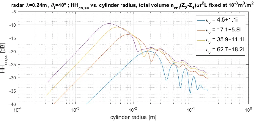
Figure 2.7. Normalized radar backscattering cross-section HH𝑐𝑛,𝑠𝑠 from equation (2.7a) at
incidence angle of 40 for a layer of uniformly randomly oriented identical cylinders, as a function of cylinder radius 𝑟 for several values of dielectric relative permittivity (blue curve: 𝜀𝑣 = 4.5 +
1.1i; red curve: 𝜀𝑣 = 17.1 + 5.8i; yellow curve 𝜀𝑣 = 35.9 + 11.1i; 𝜀𝑣= 62.7 + 18.2i). Total
volume of cylinders per unit ground area is fixed at 10−3m3/m2, and cylinder 𝐿 = (𝑟 1cm⁄ )2/3 m.
Figure 2.8. Normalized radar backscattering cross-section HV𝑐𝑛,𝑠𝑠 from equation (2.7c) at incidence
angle of 40 for a layer of uniformly randomly oriented identical cylinders, as a function of cylinder radius 𝑟 for several values of dielectric relative permittivity (blue curve: 𝜀𝑣= 4.5 + 1.1i; red curve:
𝜀𝑣 = 17.1 + 5.8i; yellow curve 𝜀𝑣 = 35.9 + 11.1i; 𝜀𝑣 = 62.7 + 18.2i). Total volume of cylinders
Even though here the cylinder length 𝐿 was fixed in relation to 𝑟 and the results for different choices for 𝐿 are not displayed, the extinction is actually independent of 𝐿, if the total volume is fixed. The reason is that cylinders with longer length have a proportionately longer extinction contribution, but the total number of cylinders is also proportionately fewer. The backscatter contribution from the canopy is also only weakly dependent on cylinder length, if the total volume is fixed. Given a fixed total volume 𝑛𝑐𝑛(𝑍2− 𝑍1)𝜋𝑟2𝐿, if 𝐿 is increased, each cylinder has a larger backscatter scaling as the square of 𝐿, but the total number of cylinders 𝑛𝑐𝑛 is inversely proportional to 𝐿, and further there are also fewer cylinders close to perpendicular to the incident direction that contribute significantly to the backscatter (within an angle proportional to 𝜆/𝐿).
From a modelling perspective, for vegetated areas, in particular forests and dense natural vegetation, the single most important parameter for the canopy volume is the total volume (per unit ground area) of resonance-sized branches. Ideally, full knowledge of the distribution of that volume as a function of cylinder radius is needed. Fractal tree models [49] and “computer-grown” trees based on architectural plant models have been used [50] for radar backscatter simulations, but these do not explicitly specify the distribution as a function of cylinder radius. Reviewing some of the radar modelling literature [9, 46, 51, 16, 15, 52], attempts have been made at measuring the distribution of branches, but a clear, simple functional form with widespread applicability for global-scale modelling has not been proposed. For that, we turn to a general model proposed by West et al. [53] in the ecology literature. While their theory is much more general, parts of which remain controversial, we only seek the distribution of branches as a function of radius, not the validity of their entire theory. Their model [53] views a plant as a “branching hierarchical network running from the trunk (level k=0) to the petioles (level k=K>0)”, with the number of branches of a given size inversely proportional to the square of the branch radius
𝑁𝑘 ∝ 𝑟𝑘−2 (2. 37)
reminiscent of an observation by Leonardo da Vinci [54]: cross-sectional area is preserved whenever a tree branches. This area-preserving branching condition was la also associated with the pipe model by Shinozaki et al. [55] [56]. The branch radii at each level are related by
𝑟𝑘+1 𝑟𝑘
= constant. (2. 38)
Extending the discrete hierarchical levels to a continuous distribution, the discrete levels can be viewed as occupying evenly spaced bins of width ∆ ln 𝑟 on a log-scale of branch radius:
𝑁𝑘 ∝ 𝐴 𝑛𝑐𝑛𝑝(𝑟) ∆ ln 𝑟 ∝ 𝑟−2 (2. 39)
𝑛𝑐𝑛𝑝(𝑟) ∝ 𝑟−3. (2. 40)
What is the range of branch radii for which this distribution is valid? There must certainly be some minimum (since the smallest branches terminate as leaves) and maximum (since there is a maximum size to branches) branch radii beyond which these relationships fail. From Shinozaki et al. [55, 56], this minimum value occurs around 1-2mm, while the maximum value depends on the tree species, since different tree species have different maximum branch sizes. Fortunately, the approximate range of validity includes the range of resonance cylinder radii (at 𝜆 = 0.24 m and 𝜀𝑣 ≈ 36 + 11i ), from 1 mm to 3 cm. Our approach for forests is thus to model the branches only up to an arbitrary cutoff maximum radius of 3 cm and down to a minimum radius of 1 mm. As mentioned earlier, the Rayleigh regime smaller than 1 mm is not expected to contribute significantly to the radar backscatter. However, for the maximum cutoff, further simulations show that the forward model does have some sensitivity to the choice of cutoff in a way that also depends on other input parameters. Hence, failure to model branches larger than 3 cm may have some detrimental impact on the accuracy of the forward model, since the true maximum branch radius may be larger than that, especially in the tropical jungles. The benefit of this simplification is the avoidance of having to handle the maximum branch size as an additional species-dependent unknown variable, which would be tricky to implement on a global scale. Additionally, 3 cm does correspond approximately to the maximum branch radius from various field measurements in boreal forests [57, 46, 52].
With the radius distribution specified, the cylinder lengths remain. Mechanical considerations and botanical data of trees are consistent with a relationship between length and radius of the form given by McMahon and Kronauer [58] :
𝐿𝑡𝑜𝑡(𝑟) ∝ 𝑟23 (2. 41)
𝐿𝑡𝑜𝑡(𝑟) = 𝐿𝑡𝑜𝑡,𝑏( if the typical ratio of the radius between a parent and daughter branch is 2, 𝑐 may be taken to be 2. 𝐿𝑡𝑜𝑡,𝑏 is potentially measurable. However our aim is to reduce the number of parameters as much as possible and it is not immediately clear what an appropriate choice of
𝐿𝑡𝑜𝑡,𝑏 and 𝑐 are, nor if they even are constants across different species of trees. The 𝑟2/3 relationship suffices for us to construct the volume distribution without requiring knowledge of 𝐿𝑡𝑜𝑡,𝑏 and c.
To recapitulate, the cylinder size distribution required for the forest canopy layer is as follows. The reference cylinder radius 𝑟𝑏 is arbitrarily fixed to be 𝑟𝑏 = 1 cm. The cylinder length 𝐿𝑏 (corresponding to reference radius 𝑟𝑏) is fixed to be 𝐿𝑏 = 1 m. The lower bound of the distribution is fixed at 𝑟𝑚𝑖𝑛,𝑏 = 1 mm. The upper bound of the distribution is chosen to be 𝑟𝑚𝑎𝑥,𝑏 = 3 cm.
The number of canopy layer cylinders per unit radius per unit ground area is of the form
𝑛𝑐𝑛𝑝(𝑟) = 𝑁𝑏(𝑟 𝑟𝑏)
−3
(2. 43)
where the scaling parameter 𝑁𝑏, with units of m−1m−2, can be thought of as describing the “density” of resonance-sized branches. Associated with each branch of radius 𝑟 is a length
nor directly measureable. What is physically meaningful, and measurable (though perhaps with tedious effort), is the volume distribution
𝑉𝑏(𝑟) = 𝑛𝑐𝑛𝑝(𝑟)𝜋𝑟2𝐿(𝑟) = 𝑁𝑏𝐿𝑏𝜋𝑟𝑏2(
𝑉𝑏(𝑟)𝑑𝑟 is to be interpreted as the total volume, per unit ground area, of branches with radius between 𝑟 and 𝑟 + 𝑑𝑟. Also measurable would be the total volume 𝑉𝑏,𝑡𝑜𝑡 per unit ground in our model controlling “amount of vegetation”.
Note that this formulation can alternatively be derived from the assumptions of area-preserving branching and the 𝐿𝑡𝑜𝑡(𝑟) ∝ 𝑟2/3 relationship in the following way: Let the total branch cross-sectional area (per unit ground area) in the area-preserving assumption be 𝐴. Then by considering a volume element,
and by comparison with earlier expression for 𝑉𝑏(𝑟), we can identify
𝑁𝑏 = 2𝐿𝑡𝑜𝑡,𝑏 3𝐿𝑏𝜋𝑟𝑏3
which reveals that 𝑁𝑏 may also be interpreted as being proportional to the stand basal area, or more accurately, the cross-sectional area at base of live crown, per unit ground area. This proportionality and interpretation, however, assumes 𝐿𝑡𝑜𝑡,𝑏 to be a known universal constant, which may not be true.
These general relationships allow us to drastically reduce the number of free parameters in the forward model, and also frees us from depending on local plot-specific empirical distributions of branch cylinder sizes. For numerical computation of the integrals (2.5) and (2.26), the cylinder radius distribution is represented using 40 log-uniform radius bins between 𝑟𝑚𝑖𝑛,𝑏and 𝑟𝑚𝑎𝑥,𝑏, and sums performed accordingly.
2.8 Distribution of cylinders in the trunk layer
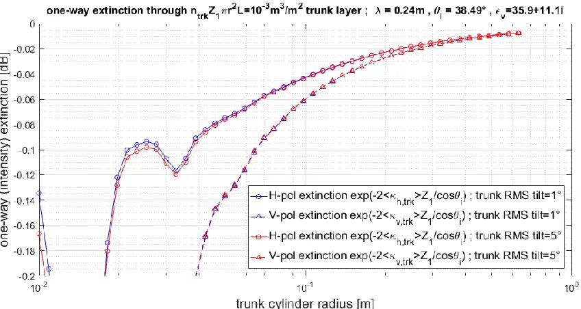
The final distribution needed is the trunk cylinder size distribution. As before, a preliminary analysis of the dependence of the forward model on the trunk cylinder radius 𝑟 is performed. This preliminary analysis is performed for a trunk layer of cylinders with their orientations following a Gaussian distribution about the vertical, as described in Section 2.5, with RMS tilt 𝜎𝑐 = 1° or 𝜎𝑐= 5°. There is no canopy layer for this preliminary trunk layer analysis (set
𝑍2 = 𝑍1). All the cylinders in the layer have identical sizes. The length, L, is chosen such that the length-to-radius ratio 𝐿 𝑟⁄ is some fixed value. The cylinder number density 𝑛𝑡𝑟𝑘 is chosen in such a way as to keep the total volume of cylinders per unit ground area
Figure 2.9. One-way extinction at incidence angle of 38.49 for the trunk layer comprising identical cylinders, as a function of trunk cylinder radius 𝑟, for trunk RMS tilt angles of 1 (blue curves) and 5 (red curves), and for h-polarization (open circles) and v-polarization (triangles). The total volume of cylinders per unit ground area 𝑛𝑡𝑟𝑘𝑍1𝜋𝑟2𝐿 is kept fixed at 10−3m3/m2.
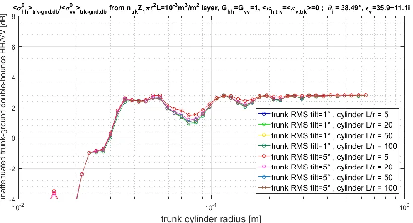
Figure 2.10. Normalized radar backscattering cross-section for the trunk-ground double-bounce HH𝑡𝑟𝑘−𝑔𝑛𝑑,𝑑𝑏 at incidence angle of 38.49 as a function of trunk cylinder radius, for various trunk
RMS tilt angles and cylinder length-to-radius ratios (see legend). No extinction was applied (pretend 〈𝜅ℎ,𝑡𝑟𝑘〉 = 〈𝜅𝑣,𝑡𝑟𝑘〉 = 0), and the ground was perfectly reflecting (set 𝐺ℎℎ= 𝐺𝑣𝑣 = 1).
Figure 2.11. Same as Figure 2.10, but for the trunk-ground double-bounce HH𝑡𝑟𝑘−𝑔𝑛𝑑,𝑑𝑏/
VV𝑡𝑟𝑘−𝑔𝑛𝑑,𝑑𝑏 ratio.
Several important observations can be made about Figure 2.9 to Figure 2.11. Firstly, as expected from the vertical orientations, the extinction is greater at v-polarization ( 〈𝜅𝑣,𝑡𝑟𝑘〉 >
with approximately the same contribution). So in this regime, the total HH𝑡𝑟𝑘−𝑔𝑛𝑑,𝑑𝑏 should increase with increasing cylinder length 𝐿 but have little dependence on the trunk RMS tilt 𝜎𝑐. On the other hand, if 𝐿 is large enough and 𝜎𝑐 is also large enough such that
𝜎𝑐 ≫ 𝜆/𝐿, not all the cylinders have a significant contribution; the fraction of cylinders having a significant contribution is inversely proportional to both 𝜎𝑐 and 𝐿. The dependence on 𝐿 thus cancels out, similar to the situation for the upper canopy layer, and the total
HH𝑡𝑟𝑘−𝑔𝑛𝑑,𝑑𝑏 is inversely proportional to the trunk RMS tilt 𝜎𝑐 in this regime.
As before for the canopy layer, the volume distribution as a function of radius is key. Even though there are fewer larger trees than smaller trees, more of the total volume in tree trunks is in the larger trees. Following West et al. [59] and Enquist et al. [60], we use an inverse square distribution for the trunk cylinder radii
𝑛𝑡𝑟𝑘𝑝𝑡𝑟𝑘(𝑟) ∝ 𝑟−2 (2. 50)
which gives a volume distribution
𝑉𝑡𝑟𝑘(𝑟) = 𝑛𝑡𝑟𝑘𝑝𝑡𝑟𝑘(𝑟)𝜋𝑟2𝐿(𝑟). (2. 51)
For the cylinder lengths, we again apply the relation (2.44)
𝐿(𝑟) = 𝐿𝑏(𝑟 𝑟⁄ )𝑏 23 (2. 52)
volume fraction of the total volume, and also to be consistent with the approximate proportionality 𝑉𝑏,𝑡𝑜𝑡 ∝ 𝑟𝑚𝑎𝑥,𝑏2/3 − 𝑟𝑚𝑖𝑛,𝑏2/3 ≈ 𝑟𝑚𝑎𝑥,𝑏2/3 (equation 2.46 for 𝑟𝑚𝑎𝑥,𝑏 ≫ 𝑟𝑚𝑖𝑛,𝑏 ) if it had been extended beyond its supposed range of validity from the branches to the whole tree. Choosing the volume fraction in branches with 𝑟 ≤ 3cm to be 𝑉𝑏,𝑡𝑜𝑡/(𝑉𝑏,𝑡𝑜𝑡 + 𝑉𝑡𝑟𝑘,𝑡𝑜𝑡) =
0.2 and solving yields a value of 𝑟𝑚𝑎𝑥,𝑡𝑟𝑘= 33.5 cm that we use as the maximum trunk radius in our model. Since the trunk extinctions and bistatic cross-sections are slowly varying when cylinder radius is large, of importance here is not so much whether 𝑟𝑚𝑎𝑥,𝑡𝑟𝑘= 33.5 cm is an accurate guess, but that we have fixed 𝑉𝑏,𝑡𝑜𝑡 to be 20% of the total volume. This 20% value is an estimate that seems consistent with that by Beaudoin et al. [51]. The other key parameter is the trunk RMS tilt 𝜎𝑐. For a reasonable guess, from Chauhan et al. [16], we expect that 𝜎𝑐< 10°. Here we use the 𝜎𝑐 = 5° guess made by Durden et al. [14], also consistent with Beaudoin et al. [51], though all these studies were only on coniferous forests.
Under these assumptions, we compute and tabulate in Table 2.1 to Table 2.5 below some quantities relevant to computing equations (2.28b-c) for the trunk-ground double reflections.
exp[−2𝑛𝑡𝑟𝑘𝑍1〈𝜅ℎ,𝑡𝑟𝑘〉/ cos 𝜃𝑖]
𝜀𝑣 = 5.15 + 1.41𝑖 𝜀𝑣 = 17.1 + 5.8𝑖 𝜀𝑣 = 35.9 + 11.1𝑖 𝜀𝑣= 62.8 + 18.2𝑖 𝜃𝑖 = 29.36° -0.042282dB -0.031799dB -0.029454dB -0.026318dB
𝜃𝑖 = 38.49° -0.053868dB -0.041922dB -0.038671dB -0.035311dB
𝜃𝑖 = 46.29° -0.066636dB -0.053518dB -0.049232dB -0.045651dB
Table 2.1. One-way h-polarization extinction exp[−2𝑛𝑡𝑟𝑘𝑍1〈𝜅ℎ,𝑡𝑟𝑘〉/ cos 𝜃𝑖] for a 𝑉𝑡𝑟𝑘,𝑡𝑜𝑡=
10−3m3m−2 trunk layer, for several values of incidence angle 𝜃𝑖 and trunk cylinder relative
permittivity 𝜀𝑣 .
exp[−2𝑛𝑡𝑟𝑘𝑍1〈𝜅𝑣,𝑡𝑟𝑘〉/ cos 𝜃𝑖]
𝜀𝑣 = 5.15 + 1.41𝑖 𝜀𝑣= 17.1 + 5.8𝑖 𝜀𝑣= 35.9 + 11.1𝑖 𝜀𝑣 = 62.8 + 18.2𝑖 𝜃𝑖 = 29.36° -0.054415dB -0.044106dB -0.046044dB -0.044469dB
𝜃𝑖 = 38.49° -0.070223dB -0.058606dB -0.060656dB -0.059221dB
𝜃𝑖 = 46.29° -0.087169dB -0.074483dB -0.076645dB -0.075310dB
16𝜋𝑛𝑡𝑟𝑘𝑍1〈|𝑆ℎℎ|𝑡𝑟𝑘,3𝑎2 〉/𝑘2
𝜀𝑣 = 5.15 + 1.41𝑖 𝜀𝑣= 17.1 + 5.8𝑖 𝜀𝑣= 35.9 + 11.1𝑖 𝜀𝑣 = 62.8 + 18.2𝑖 𝜃𝑖 = 29.36° -10.9376dB -10.7324dB -10.1299dB -9.9533dB
𝜃𝑖 = 38.49° -12.5545dB -10.8279dB -10.0889dB -9.7269dB
𝜃𝑖 = 46.29° -13.5699dB -10.9303dB -10.1317dB -9.6721dB
Table 2.3. Hypothetical normalized radar cross-section at h-polarization 16𝜋𝑛𝑡𝑟𝑘𝑍1〈|𝑆ℎℎ|𝑡𝑟𝑘,3𝑎2 〉/
𝑘2 for a 𝑉
𝑡𝑟𝑘,𝑡𝑜𝑡= 10−3m3m−2 trunk layer with perfectly reflecting ground and without extinction
considerations, for several values of incidence angle 𝜃𝑖 and trunk cylinder relative permittivity 𝜀𝑣.
16𝜋𝑛𝑡𝑟𝑘𝑍1〈|𝑆𝑣𝑣|𝑡𝑟𝑘,3𝑎2 〉/𝑘2
𝜀𝑣 = 5.15 + 1.41𝑖 𝜀𝑣= 17.1 + 5.8𝑖 𝜀𝑣= 35.9 + 11.1𝑖 𝜀𝑣 = 62.8 + 18.2𝑖 𝜃𝑖 = 29.36° -23.0373dB -17.1299dB -13.7693dB -12.2022dB
𝜃𝑖 = 38.49° -20.3795dB -14.5201dB -12.2302dB -11.0765dB
𝜃𝑖 = 46.29° -18.1205dB -13.3495dB -11.5116dB -10.5306dB
Table 2.4. Same as Table 2.3, but for v-polarization 16𝜋𝑛𝑡𝑟𝑘𝑍1〈|𝑆𝑣𝑣|𝑡𝑟𝑘,3𝑎2 〉/𝑘2.
〈|𝑆ℎℎ|𝑡𝑟𝑘,3𝑎2 〉/〈|𝑆𝑣𝑣|𝑡𝑟𝑘,3𝑎2 〉
𝜀𝑣 = 5.15 + 1.41𝑖 𝜀𝑣= 17.1 + 5.8𝑖 𝜀𝑣= 35.9 + 11.1𝑖 𝜀𝑣 = 62.8 + 18.2𝑖 𝜃𝑖 = 29.36° 12.0996dB 6.3975dB 3.6395dB 2.2489dB
𝜃𝑖 = 38.49° 7.8249dB 3.6923dB 2.1413dB 1.3496dB
𝜃𝑖 = 46.29° 4.5506dB 2.4192dB 1.3800dB 0.8585dB
Table 2.5. Same as Table 2.3, but for the ratio 〈|𝑆ℎℎ|𝑡𝑟𝑘,3𝑎2 〉/〈|𝑆
𝑣𝑣|𝑡𝑟𝑘,3𝑎2 〉.
C h a p t e r 3
APPLICATION OF L-BAND RADAR BACKSCATTER MODEL TO
AQUARIUS DATA OVER GLOBAL FORESTS
3.1 Chapter overview
In this chapter, our L-band radar backscatter model shall be compared with the data from the spaceborne L-band scatterometer of Aquarius. The Aquarius mission is unique for having had both significantly long temporal coverage (slightly more than 3 years), frequent (weekly) repeat global coverage, and a L-band scatterometer with high accuracy and stability (<0.2dB) at all polarization channels [61, 62, 63]. Frequent repeats are important for studying changes in ground moisture, which may rise rapidly with precipitation in a matter of hours, and then dry down on a time scale of days.
In subsequent sections (Sections 3.3-3.7) of this chapter, the comparison between our L-band radar backscatter model and the data from the Aquarius scatterometer will be performed class-by-class for the five forest classes, with reference to the global land cover classes of the International Geosphere-Biosphere Programme (IGBP) [35], bearing in mind the coarse 100km spatial resolution and 7-day temporal resolution. Physically reasonable
distribution for the canopy cylinders was more suited for needleleaf forests, a uniformly random orientation distribution was more suited for broadleaf forests, and mixed forests somewhere in between. Sensitivity to sub-canopy flooding and differences between frozen/unfrozen states was expected [66, 67] and our model provides partial quantitative agreement by modelling them in terms of changes in ground surface roughness, ground dielectric relative permittivity, and vegetation dielectric relative permittivity; the frozen/unfrozen comparison will be in Section 3.8. Microwave vegetation optical depth values will be reported in Section 3.9.
3.2 Input datasets
The Aquarius/SAC-D mission was launched in 2011 with the primary goal of measuring sea surface salinity from space. Here we use the portion of data that was taken over land. The instrument carried 3 radiometers operating at 1.41GHz, with beams at incidence angles of about 29, 38, and 46. It also carried a scatterometer at 1.26GHz that shares the feed horns with the radiometers. The scatterometer measured, for each incidence angle, normalized radar backscattering cross-sections HH, HV, VH, and VV, with footprints 100km. Further instrument details can be found in Le Vine et al. [61], Fore et al. [62], and Yueh et al. [68]; in particular, Fig. 3 from the paper by Le Vine et al shows a schematic of the radiometer and scatterometer footprints of the 3 beams, reproduced here in Figure 3.1.
referred to as EASE2 grid pixels). This regridding reassigns data based on which EASE2 grid pixel the centre of each radar footprint was nearest to. Note that the footprint size is significantly larger than the pixel size.
Figure 3.1. Aquarius 3-dB footprints and swath of the three beams for radiometer (solid lines) and scatterometer (dashed lines), as shown in Fig. 3. of Le Vine et al. [61] © IEEE 2007
Some swath and regridding artefacts are visible in Figure 3.2, but these artefacts should have little impact on the comparison with the model and the inferences drawn.
Figure 3.2.