Estimation of stochastic volatility models via Monte Carlo maximum likelihood

*Corresponding author. E-mail: [email protected]

Estimation of stochastic volatility models

via Monte Carlo maximum likelihood

Gleb Sandmann!, Siem Jan Koopman",*

!Financial Markets Group, London School of Economics and Political Science, Houghton Street, London WC2A 2AE, UK

"CentER for Economic Research, Tilburg University, 5000 LE Tilburg, Netherlands

Received 1 September 1996; received in revised form 1 October 1997

Abstract

This paper discusses the Monte Carlo maximum likelihood method of estimating stochastic volatility (SV) models. The basic SV model can be expressed as a linear state space model with log chi-square disturbances. The likelihood function can be approxi-mated arbitrarily accurately by decomposing it into a Gaussian part, constructed by the Kalman filter, and a remainder function, whose expectation is evaluated by simulation. No modifications of this estimation procedure are required when the basic SV model is extended in a number of directions likely to arise in applied empirical research. This compares favorably with alternative approaches. The finite sample performance of the new estimator is shown to be comparable to the Monte Carlo Markov chain (MCMC) method. ( 1998 Elsevier Science S.A. All rights reserved.

JEL classification: C15; C22

Keywords: GARCH model; Importance sampling; Kalman filter smoother; Monte Carlo simulation; Quasi-maximum likelihood; Stochastic Volatility; Unobserved components

1. Introduction

The empirical distributions of financial time series differ substantially from distributions obtained from sampling independent homoskedastic Gaussian variables. Unconditional density functions exhibit leptokurtosis and skewness;

0304-4076/98/$—see front matter₍ 1998 Elsevier Science S.A. All rights reserved.

1The Quasi-Maximum Likelihood (QML) method of Harvey et al. (1994), and GMM methods of Andersen and S₊rensen (1996) are examples of this category.

time series of stock returns show evidence of volatility clustering; and squared returns exhibit pronounced serial correlation whereas little or no serial depend-ence can be detected in the return process itself. These empirical regularities suggest that the behavior of financial time series may be captured by a model which recognizes the time varying nature of return volatility, as follows:

R

t"k

t#p

tet, et&IID (0,1), t"1,₂,¹

whereR

tdenotes the return on an asset. One way of modellingptis to express

it as a deterministic function of lagged residuals, r

t"R

t!k

t. Econometric

specifications of this form are known as ARCH models and have achieved widespread popularity in applied empirical research (Bollerslev et al., 1992; Bollerslev et al., 1993; Bera and Higgins, 1993). Alternatively, volatility may be modelled as an unobserved component following some latent stochastic process, such as an autoregression. Models of this kind are known as stochastic volatility (SV) models (Taylor, 1994; Ghysels et al., 1996; Shephard, 1996).

Despite their intuitive appeal, SV models have been used less frequently than ARCH models in empirical applications. This is due to the difficulties associated with the estimation of SV models. Unlike ARCH models, where the likelihood function can be evaluated exactly, the likelihood function of an SV model is hard to construct. Existing estimation procedures can be subdivided into two groups: (i) methods that attempt to build the full likelihood function, and (ii) methods

which rely on alternative, usually less efficient principles.1

Several propositions have been made as to how the full likelihood function may be evaluated. Kim et al. (1996) show how the likelihood can be constructed when a mixture of normals is used to approximate the density of the distur-bances. Jacquier et al. (1994) have proposed a Bayesian approach to the estimation of SV models using the Monte Carlo Markov chain (MCMC) technique. Fridman and Harris (1996) show how the extended Kalman filter can be used to perform numerical integration. Finally, Danielsson (1994a) suggested that accurate approximations to the likelihood function can be obtained by means of importance sampling.

Recently, Shephard and Pitt (1997) and Durbin and Koopman (1997, 1998) designed methods for constructing the likelihood function for general state space models using Monte Carlo simulation techniques; thereafter referred to as Monte Carlo likelihood (MCL). This paper shows how the general concepts can be implemented efficiently for the standard linear SV model and for a variety of SV model extensions. The properties of the MCL estimates are compared with other approaches by using Monte Carlo experiments and empirical illustrations. The crucial feature of the MCL approach is the formulation of the SV model

equation. The question of how to treat zero observations — which will

make ln(r2

t) ill-defined — is addressed explicitly. The linear state space

form allows very powerful algorithms for filtering and smoothing to be utilized, and more generally, to draw upon a vast body of knowledge on structural time series models (Harvey, 1989). The gain is also due to the elegant form of the likelihood specification as put forward by Durbin and Koopman (1997) in which the log likelihood is the sum of the Gaussian log likelihood (i.e. QML) and a correction for the departures from Gaussian assumptions. Monte Carlo simulation is only employed to construct the correction part of the likelihood function.

Apart from reducing the computational effort considerably (while attaining finite sample efficiency), the algorithm has several distinct advantages. First, the sampling variation can be reduced giving arbitrarily close approximations to the true likelihood function value. Thus standard likelihood ratio tests can be constructed. This is likely to be very useful since numerical standard errors of model parameters often leave much to be desired.

Secondly, a wide range of extensions can be addressed with trivial modifica-tions of the estimation procedure due to the fact that the state space form is retained. Thus, several well-known extensions of the basic SV model can be examined: fat tailed distributions for the mean equation disturbances, SV in the mean specification, correlated return and volatility processes, as well as stochas-tic seasonal components, effects of dummy and exogenous explanatory variables may be explored in detail.

The paper is organized as follows. Section 2 discusses in more detail the various aspects of estimation and inference in the context of SV models. In Section 3 we describe the Monte Carlo likelihood (MCL) estimation method while Section 4 compares its finite sample performance with existing techniques by means of an extensive Monte Carlo experiment and some empirical data examples. Section 5 illustrates how the method can be applied to the estimation of models with fat-tails, explanatory variables and non-zero correlation. Sec-tion 6 concludes.

2. Stochastic volatility model

Consider the stochastic volatility model:

r

tis the mean adjusted return on an asset. Since many financial

time series exhibit little or no dynamic behavior in the mean, but pronounced

serial dependence in the variance (Bollerslev et al., 1992) the estimation ofk

twill

2Thus the logarithm of variance follows a discrete time analog of the Orstein—Uhlenbeck process often used in the context of option pricing (Hull and White, 1987; Renault and Touzi, 1996).

denoted byp_N, and the mean and variance equation disturbancese

tandgtmay be

contemporaneously correlated.

Despite a very parsimonious representation, this model captures most of the empirical regularities found in financial time series (Ghysels et al., 1996). An attractive feature of specification (1) is the possibility of linearizing the model. By

taking logarithms of the squared mean adjusted returns one obtains2:

lnr2

If the original mean equation disturbance,m_t, is standard normal,e_tfollows the

ln(s21) distribution whose mean and variance are known to be!1.27 andn2/2,

respectively. Notice, that once the transformation is accomplished, the

informa-tion regarding the correlainforma-tion coefficient, o is lost, but can be recovered by

conditioning on the signs of the original observations (Harvey and Shephard,

1996). Estimation ofo is addressed in Section 5.4.

Harvey et al. (1994) suggested a Quasi-Maximum Likelihood (QML) method of estimating the model based on the Kalman filter. Assuming joint conditional

normality of (e

t,gt), Eq. (2) represents the measurement and transition equations

of the general linear state space model, details of which can be found in the Appendix A. Once the model is in the state space form, the advantages of this approach become evident: (i) explanatory variables can be easily incorporated into the variance equation, (ii) more general ARMA processes can be assumed for the evolution of the latent variable, (iii) missing or irregularly spaced observations can be handled, and (iv) generalisations to the multivariate case are straightforward.

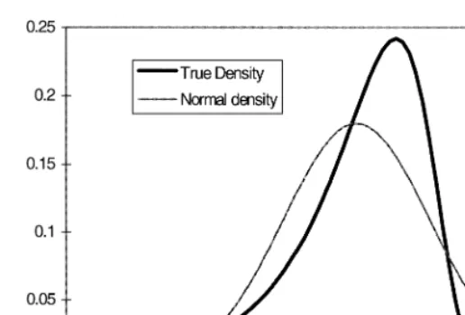
The QML method approximates the distribution of e_t by N(!1.27,p2/2),

whilee

t is far from being Gaussian. In fact, its density is given by

p

tdeviates from its normal approximation which implies

that the QML estimator is likely to have poor small sample properties even though it is consistent. Note the high degree of skewness and the long tail in the

negative half-line. Large negative values reflect inliers inr

t, which may arise in

empirical applications with high frequency data.

Fig. 1. The ln(s21) density and the normal approximation N(!1.27,p2/2).

S+rensen (1996), among others. MM estimators avoid the problem associated

with the linearization of the model as well as the evaluation of the likelihood. They are not difficult to implement and to generalize but the efficiency of these estimators is known to be suboptimal to the likelihood-based method of

inference (Jacquier et al., 1994; Andersen and S+rensen, 1996). Gallant and

Tauchen (1996) have developed a MM procedure which matches the scores of an auxiliary model via simulation (SMM). They claim that, if the auxiliary model is a good approximation to the distribution of the data, the MM estimator is as efficient as maximum likelihood. However, none of the MM estimation methods

provide an estimate of the instantaneous volatilityp2

t throughout the sample,

t"1,₂,¹, so that an additional form of estimation is required. For instance, Andersen (1994) and Ghysels and Jasiak (1996) use MM techniques to estimate the parameters and they use the Kalman filter to obtain volatility estimates.

Secondly, Kim et al., (1996) suggest to approximate the distribution ofe

tby

a mixture of normals. Given a particular mixture, the likelihood can be com-puted via the prediction error decomposition since the linear structure of the model is essentially retained. An important drawback of this method is that no matter how many mixture components are used, the mixture of normals cannot

give a good approximation to the tail behavior of the ln(s2) distribution. In

addition, the convergence of the algorithm is likely to be very sensitive to the number and weight of individual mixture components (Jacquier et al., 1994).

Thirdly, Fridman and Harris (1996) suggest that the non-Gaussianity of the measurement equation disturbances can be handled by means of a ‘brute force’

numerical integration. In a Monte Carlo study—similar to the one presented

can be applied in this context. By retaining the state space form, Fridman and Harris (1996) estimation technique offers the same advantages as the MCL. Some of the disadvantages of this method consist of computational inefficiencies (the extended Kalman filter is known to be rather slow) and the necessity to choose a priori a fixed grid, over which the volatility process will be integrated. This creates a trade-off between numerical accuracy on the one hand, and computational efficiency on the other. It is conceivable, that in some instances an optimal grid may not exist. For instance, when estimating the volatility process around the stock market Crash of ’87 the grid selection procedure proposed by Fridman and Harris (1996) will either lead to a very coarse grid over the entire volatility range, or place no probability weight on the high-volatility state during the Crash.

A Bayesian approach to the estimation of SV models using a Monte Carlo Markov chain (MCMC) technique was developed by Jacquier et al. (1994), JPR thereafter. They have performed extensive simulation experiments which dem-onstrate that MCMC is superior to QML and MM estimation techniques across a wide range of parameter values. However, this technique has some undesirable features. The procedure is quite involved, requiring a large amount of computer intensive simulations. In addition, the method needs to be nontrivially modified for the extensions like the introduction of explanatory variables, alternative processes for the evolution of variance, or multivariate specifications (Jacquier et al., 1995). Shephard and Pitt (1997) have constructed an efficient block MCMC algorithm for performing Bayesian inference on general nonlinear and non-Gaussian state space models of which the SV model (1) is a special case. They conclude that the performance of the multiblock MCMC methods outperforms the single block approach of JPR in terms of computational efficiency.

Finally, Danielsson (1994a) proposed to estimate the SV model by the Monte Carlo likelihood (MCL) estimation method. His accelerated Gaussian impor-tance sampler (AGIS) algorithm is a simulation-based technique whose time requirement and precision is on par with MCMC. However, the method is difficult to generalize and remains computationally expensive largely due to the failure of the technique to exploit the linear structure resulting from the trans-formation (2).

of Likelihood Ratio test statistics because the likelihood function can be ap-proximated arbitrarily close.

3. Monte Carlo Maximum likelihood estimation

3.1. The general algorithm

Taking logarithms of the squared residuals in Eq. (1), that isy_t"ln(r2

t), gives

the SV model in the linear state space form (2) but invokes an additional difficulty: the disturbance term in the measurement equation becomes non-Gaussian. The Appendix A discusses the general linear state space model and the associated algorithms for filtering, smoothing and simulation. The Monte Carlo likelihood (MCL) approach for non-Gaussian models such as the SV model is based on importance sampling techniques (Ripley, 1987). Danielsson (1994a) and Shephard and Pitt (1997) consider generating samples from an approximating Gaussian model. Durbin and Koopman (1997) demonstrate that the log likelihood function of state space models with non-Gaussian measure-ment disturbances can be simply expressed as

ln¸(yD t)"ln¸

function of the approximating Gaussian model,p

536%(eDt) is the density function

of the measurement disturbances, that is the ln(s21) density in the case of the basic

SV model,p

G(eDt) is the Gaussian density of the measurement disturbances of

the approximating model and E

G refers to expectation with respect to the

so-called importance density p

G(eDy,t) associated with the approximating

model. Eq. (4) reveals that only importance samples are required for the

measurement disturbancese"(e

1,e2,2,e

T)@. Furthermore, Eq. (4) shows that

the non-Gaussian log likelihood function can be expressed as the log likelihood function of the Gaussian approximating model plus a correction for the depar-tures from the Gaussian assumptions in relation to the true model. The unbiased estimate of Eq. (4) is given by:

ln¸K(t)"ln¸

G(yDt)#lnwN# s2w

2NwN2 (5)

wherew_N ands2

ware computed by the algorithm of Durbin and Koopman (1997):

1. Choose a Gaussian approximating model from which a feasible sampling

scheme can be deducted based on the importance density p

G(eDy,t); see

3A similar suggestion is made by Shephard and Pitt (1997) but their argument is based on finding an approximating Gaussian model which produces posterior mode estimates for the true model.

2. Compute (and store) ln¸

G(yDt) and eL"E(e Dy,t) for the approximating

model via the Kalman filter smoother; see Appendix A for details.

3. Generate a samplee(i)"(e(i)

1,2,e(i)

T)@from the importance densitypG(e Dy,t)

referring to the approximating model of step 1. A specific version of the simulation smoother of de Jong and Shephard (1995) is used to generate this sample; see Appendix A for details.

4. Construct an antithetic sample:eJ(i)"2eL!e(i).

6. Repeat steps 3—5 untilNsamples are drawn.

7. CalculatewN ands2

was the sample mean and variance ofw(i),i"1,₂,N.

The MCL estimates of model parameters, t are obtained by numerical

optimization of Eq. (5). The log likelihood function of the approximating model,

ln¸

G(yD t), can be used to obtain starting values. The choice ofNgoverns the

accuracy of the approximation to the likelihood function: as N increases, the

approximation becomes more accurate. For practical purposes we find that

N"5 is sufficient; see the detailed discussion in Section 4 below.

3.2. Implementation

The importance sampling densityp_G(e Dy,t), could be based on the

approxi-mating SV model as given by Eq. (2) with e_t&N(0,H

t) where Ht"n2/2, for

t"1,₂,¹. However, Durbin and Koopman (1997) argue that a better

import-ance density is obtained from Eq. (2) withe

t&N(0,HI

t) where the scalar

vari-ancesH_I

t’s are chosen so as to make the differences between the log densities

lnp

-/s21(e D t) and lnp_G(e D t) as constant as possible in the neighbourhood of eL"E(e Dy,t).3The smoothed error vectoreL"(eL

1,2,eL

T)@ is calculated by the

Kalman filter smoother. Details of which can be found in the Appendix.

Intuitively, large negative values ofeL

twould require high values ofHI tin order

for the slopes of the densities in Fig. 1 to be roughly equal, fort"1,₂, T. The

choice of the variances HI

t’s of the approximating model is determined by

equalizing the derivatives of the log densities ateL:

12(1!ee)

K

e/eL

"!e

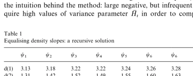
Table 1

Equalising density slopes: a recursive solution

t₁ t₂ t₃ t₄ t₅ t₆ t₆ t₈ t₉ iterations of the simulated SV model with ¹"_{1000 and across several parameter triplets}

t_i"₍p

g,/,a)i, the values of which are reported in Table 2. Small values ofd(k) indicate that the

individual elements of the variance vectorHI are not changing considerably across further iterations, i.e.HI(_tk)P_HM

t.

where the left-hand side is the derivative of Eq. (3) and the right-hand side is the

derivative of the Gaussian density. This leads to a set of¹equations:

HI

t" 2eLt

eeLt!1 t

"1,₂,¹. (6)

Note that Eq. (6) ensure the nonnegativity of HI

t since the numerator and

denominator are of the same sign for any value ofeL

t. The set of nonlinear Eq. (6)

is solved forHI

tby iteration, starting atHI (0)t "n2/2∀t. Given a parameter vector

t, we iterateKtimes between computingeL

t(using the Kalman filter smoother)

and computing HI (_tk) by Eq. (6), fork"1,₂,K. This procedure is performed

only once in Step 1 of the algorithm of Section 3.1. Naturally, when the

parameter vectortchanges, the algorithm needs to be repeated.

Table 1 shows rapid convergence results across a range of parameter values

for the simulated SV model. Choosing the metricd(k)"¹~1+

tDHI (tk)!HI (k~1)

t Dto

describe successive changes in the variance vector,H_I , we find that after about

six-to-eight iterations the elements of the variance vector cease to fluctuate, i.e.

HI (k)

i PHM

t. The individual elements of the variance vector HM are now different

acrosst"1,₂,¹.

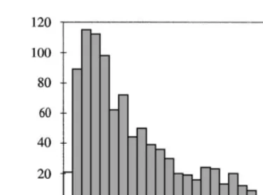
Fig. 2 is a histogram ofHM

t’s from a simulated SV process (¹"1000) governed

by a set of parameters t₅"(pN,/,p

g)5, the numerical values of which are

discussed in Section 4. It is the mirror image of the density ofe

tand reconfirms

the intuition behind the method: large negative, but infrequent values ofe

t

Fig. 2. Effect of equalizing density slopes.

difference in density slopes in this region. The converse is represented by large

probability mass ofH_M

tor less thann2/2.

Step 3 of the algorithm in Section 3.1 is accomplished by the simulation smoother of de Jong and Shephard (1995). Details of this can be found in the Appendix. We like to point out that, once the SV model is formulated in the state space form, the Kalman filter smoother and the simulation smoother are invariant to possible extensions of the basic SV model.

The quantityw(e) for the basic SV model is calculated as:

w(e)"<T

t/1

w(e_t)"exp

G

t/1

l(e_t)

H

and

l(e

t)"lnw(e

t)"12

A

t#e

t!eet#e2t

HI

t

B

(7)

whereHI

tis the variance of the measurement disturbance of the approximating

model, fort"1,₂,¹. In practicew(e(i)) is a very small number and, therefore,

appropriate scaling is required for numerical stability. Note that w(e(i)) is the

ratio of the true density of the disturbances—ln(s21)—to the Gaussian density. Its

expectation (estimated as the sample average ofw(i)’s in Step 5 of the Algorithm)

gives that part of the likelihood surface which is not already captured by the Gaussian approximation. The bias correction in Eq. (5) is due to the considera-tion of the log likelihood funcconsidera-tion rather than the likelihood funcconsidera-tion itself.

3.3. Smoothing thevolatility process

4Reflecting the difference between the Bayesian approach and the classical approach in statistics.

the GARCH models—where knowledge of the model parameters is sufficient to

construct the volatility figures recursively — in the SV framework the latent

volatility can only be estimated. Furthermore, unlike in the Bayesian MCMC

framework—where the joint density of latent volatilities and model parameters

is readily available—in the MCL method the estimated parameters are treated

as fixed for the purposes of estimating volatility via the Kalman filter smoother.4

The linear Kalman filter smoother does not explicitly take account of the non-Gaussianity in the measurement equation. However, when the Kalman filter smoother is applied to the approximating Gaussian SV model, it is effectively computing the posterior mode estimates of the volatility (Shephard and Pitt, 1997; Durbin and Koopman, 1998). If the posterior mean is required, Durbin and Koopman (1998) show that a computationally efficient algorithm is given by

t@Tis the volatility estimate,e(ti)is a draw from the importance density as

computed by the simulation smoother (see Step 3 of the algorithm of

Sec-tion 3.1),w(e(i)

t )"expMl(e(i)

t )Nis defined in Eq. (7) andwNt"(1/N)+Ni

/1w(e(ti)). The

weights f_t can be interpreted as the corrections for non-Gaussianity in the

measurement equation. It is worth stressing that Eq. (8) requires little additional

computing because the quantities e(_ti) and w(e(i)

t ) are already evaluated by the

algorithm of Section 3.1.

Finally, the estimation error,h

t@T!h

t(wherehtdenotes the true volatility) is

O(1) which implies that treating exp(h

t@T) as lognormal may lead to distortions

(Harvey and Shephard, 1993). These authors consider the following estimate of the volatility process:

pJ2_t"pN2

Teht@T, pN2T"¹~1+T

t/1

r2_te~ht@T, t"1,₂,¹ (9)

where the smoothed signal,h

t@Tis obtained from Eq. (8). Thus the estimation of

model parameters and the values of the latent volatility process are addressed simultaneously in the MCL framework.

4. Finite sample performance

4.1. Simulation experiment

comparison with the MCMC method. The range of parameter values

t"(pN,/,p

g) is selected in the following manner. First, the values of the

autoregressive parameter / are set to 0.90, 0.95, and 0.98. This choice is

motivated by empirical studies which reported the values of the autoregressive coefficient close to unity, ranging between 0.9 and 0.995. Secondly, for each

value of/, the values ofp

gare selected so that the coefficient of variation:

C»"var(h)

E[h]2"exp

A

p2_g

1!/2

B

!1

takes the values 10, 1, and 0.1. High values of the ratio of volatility variance to its squared mean indicate pronounced relative strength of the stochastic volatility

process while low values of C»signify that the model is close to the one of

constant volatility. In fact, if preliminary exploratory analysis of the data from

a model with low C» (C»"0.1) was based only on the autocorrelation

structure ofr2

t or ln(r2t) the practitioner without a strong prior belief that the SV

model is the correct specification will be unable to distinguish between the SV

and a homoskedastic model. Nevertheless, the parameter triplets t

7—t9 are included for completeness. The focus of interest is thus centered around

para-meter tripletst

4—t6which correspond to the coefficient of variation close to

unity. Most of the empirical studies surveyed by JPR report parameter estimates

in this range. Finally, the values of the location parameter,pN are chosen such

that the expected variance

E[h]"pN2exp

A

2(1!/2)

B

is set to 0.0009. If the simulated data are regarded as weekly returns, this corresponds to approximately 22% annualized variance. Note that JPR chose

a slightly different parameterization of the SV model (r

t"e(1@2)hte

values of which are reported in Table 2 in the row labelled ‘¹rue’. For eacht

iwe

generate samples of length¹"500, we estimate the model via MCL and via

QML and we compute means, standard deviations and mean squared errors of

the parameter estimates overK"500 simulated realisations of the process. In

these calculations the number of drawsNused in the algorithm of Section 3.1 is

set toN"5.

Results from the sampling experiments are presented in Table 2 which is

divided into three panels in accordance with the coefficient of variationC».

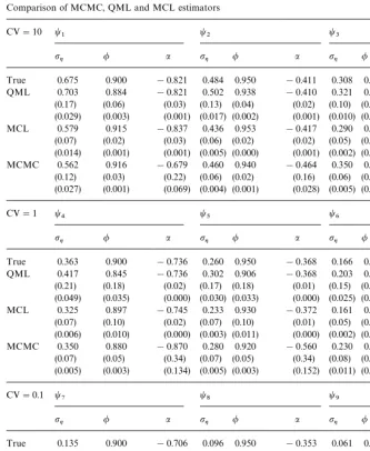
Table 2

Comparison of MCMC, QML and MCL estimators

CV"₁₀ t

1 t2 t3

p_g / a p_g / a p_g / a

True 0.675 0.900 !_{0.821 0.484 0.950} !_{0.411 0.308 0.980} !_0.164 QML 0.703 0.884 !_{0.821 0.502 0.938} !_{0.410 0.321 0.970} !_0.164 (0.17) (0.06) (0.03) (0.13) (0.04) (0.02) (0.10) (0.03) (0.01) (0.029) (0.003) (0.001) (0.017) (0.002) (0.001) (0.010) (0.001) (0.000) MCL 0.579 0.915 !_{0.837 0.436 0.953} !_{0.417 0.290 0.977} !_0.166

(0.07) (0.02) (0.03) (0.06) (0.02) (0.02) (0.05) (0.02) (0.01) (0.014) (0.001) (0.001) (0.005) (0.000) (0.001) (0.002) (0.000) (0.000) MCMC 0.562 0.916 !_{0.679 0.460 0.940} !_{0.464 0.350 0.980} !_0.190

(0.12) (0.03) (0.22) (0.06) (0.02) (0.16) (0.06) (0.01) (0.08) (0.027) (0.001) (0.069) (0.004) (0.001) (0.028) (0.005) (0.000) (0.007)

CV"₁ t

4 t5 t6

p_g / a p_g / a p_g / a

True 0.363 0.900 !0.736 0.260 0.950 !0.368 0.166 0.980 !0.147 QML 0.417 0.845 !_{0.736 0.302 0.906} !_{0.368 0.203 0.942} !_0.147 (0.21) (0.18) (0.02) (0.17) (0.18) (0.01) (0.15) (0.16) (0.01) (0.049) (0.035) (0.000) (0.030) (0.033) (0.000) (0.025) (0.029) (0.000) MCL 0.325 0.897 !_{0.745 0.233 0.930} !_{0.372 0.161 0.970} !_0.148

(0.07) (0.10) (0.02) (0.07) (0.10) (0.01) (0.05) (0.07) (0.01) (0.006) (0.010) (0.000) (0.003) (0.011) (0.000) (0.002) (0.004) (0.000) MCMC 0.350 0.880 !_{0.870 0.280 0.920} !_{0.560 0.230 0.970} !_0.220

(0.07) (0.05) (0.34) (0.07) (0.05) (0.34) (0.08) (0.02) (0.14) (0.005) (0.003) (0.134) (0.005) (0.003) (0.152) (0.011) (0.001) (0.025)

CV"0.1 t

7 t8 t9

p_g / a p_g / a p_g / a

True 0.135 0.900 !_{0.706 0.096 0.950} !_{0.353 0.061 0.980} !_0.141 QML 0.319 0.350 !_{0.706 0.295 0.420} !_{0.353 0.266 0.449} !_0.141 (0.31) (0.63) (0.01) (0.30) (0.62) (0.01) (0.30) (0.64) (0.00) (0.132) (0.702) (0.000) (0.131) (0.669) (0.000) (0.133) (0.692) (0.000) MCL 0.156 0.443 !_{0.709 0.136 0.526} !_{0.355 0.113 0.572} !_0.142

(0.11) (0.62) (0.01) (0.10) (0.60) (0.01) (0.10) (0.60) (0.00) (0.012) (0.592) (0.000) (0.012) (0.545) (0.000) (0.013) (0.524) (0.000) MCMC 0.150 0.780 !_{1.540 0.120 0.840} !_{1.120 0.140 0.910} !_0.660

(0.08) (0.19) (1.35) (0.07) (0.16) (1.15) (0.10) (0.12) (0.83) (0.007) (0.051) (2.518) (0.006) (0.038) (1.911) (0.016) (0.019) (0.958)

Note: This table reports the results of the simulation experiments. For each set of parameter tripletst_i"₍p

parameter values for both, the QML and MCL optimization routines are obtained from a two-dimensional grid search procedure which searches for an

optimum across the surface of the Gaussian log likelihood function ln¸

G(t).

The figures presented in Table 2 allow several conclusions to be drawn. The experiment demonstrates that the MCL estimator exhibits similar efficiency as

the MCMC estimator across most parameter values. For the C»"10 and

C»"1 the mean squared errors on all parameters (except for/whenC»"1)

are smaller for the MCL. When C»"1 the mean squared errors on / are

slightly larger, but the estimator exhibits lower bias (alas larger sample vari-ance).

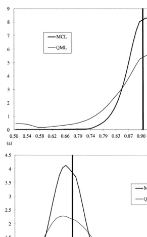
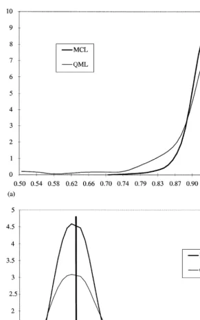
The QML estimator is found to be inefficient, thereby confirming the results

of JPR. Figs. 3 and 4 present the smoothed densities of the estimates of/and

p_gfor two tripletst₄andt₅. The MCL estimator is shown to exhibit a much

tighter sampling distribution then the QML estimator, a property also indicated by smaller standard errors of the estimates.

Across the entire parameter space the standard errors of the QML estimator are at least twice the size of the fully efficient MCL estimator while the bias is nonnegligible. The efficiency of the QML estimator increases as the strength of

the SV process becomes more pronounced. For instance, for C»"10 the

sample standard error on /"0.95 is 0.04 while in the case of C»"1 the

standard error on/"0.95 increases fourfold to 0.18.

However, although we find QML to be inefficient, its performance is nowhere as near as bad as reported by JPR. Same conclusion was reached by Breidt and Carriquiry (1996) who also re-examined the final sample performance of the QML estimator. Since Figs. 3 and 4 were constructed so as to correspond to JPR’s Figs. 4 and 5, respectively, direct comparison reveals dramatic differences in the performance of the same estimation technique. This raises the question of possible inefficiencies in JPR’s QML estimation method such as poor starting values, different convergence criteria, or inefficient implementation of the algorithm.

We also find that the performance ofall three estimatorsdeteriorates asC»

decreases. Comparison of the MCL and the MCMC estimators in this region (C»"0.1) reveals that the MCL estimates of the long-run volatility levela(i.e.

pN) are more efficient, but those ofp

gand/are less efficient than the

correspond-ing MCMC estimates. This can be explained by the fact that the dynamic properties of the model are so weak (or the signal-to-noise ratio so small) in this region that the data appear almost indistinguishable from a constant volatility model.

The performance of the estimator is examined in cases when larger data sets are available, results of which are presented in Table 3. For each of the

para-meter triplets t₄—t

6 (corresponding to C»"1) K"500 samples of length

Fig. 3. Sampling distributions of MCL and the QML estimators; (a) /"0.9;t

4, (b) pg"0.363;

Fig. 4. Sampling distributions of MCL and the QML estimators; (a) /"0.95;t

5, (b) pg"0.260;

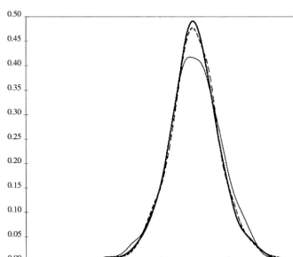
Fig. 5. S&P500: unconditional density and the density of the SV-tmodel.

5The results onN"_{5 are reproduced from Table 2, in greater detail.}

reduced. Comparison with MCMC (alas based only ont

4) reveals that the finite

sample efficiency is very similar. The mean squared errors are of the same order

of magnitude: with the MSE onp

glarger, the MSE on/identical, and MSE on

a(i.e. p_N) being smaller.

As the number of drawsNincreases, the expectation of the MCL likelihood

function (5) can be calculated more precisely, thus leading to increased perfor-mance. On the other hand the computational burden needs to be taken into

account. In our experience, a very small number of draws (N"5) is sufficient to

produce results comparable with the MCMC estimator while little can be

gained by increasingNfrom 20 to 40. This is illustrated in Table 4. We revert to

the original simulation study design of ¹"500 observations (with K"500

realisations of the process) and re-estimate the model for the central parameter

Table 3

Finite sample performance at sample length of¹"₂₀₀₀ CV"1 t

4 t5 t6

p_g / a p_g / a p_g / a

True 0.363 0.900 !0.736 0.260 0.950 !0.368 0.166 0.980 !0.147 QML 0.381 0.888 !0.736 0.268 0.945 !0.368 0.167 0.978 !0.147 (0.10) (0.05) (0.01) (0.06) (0.03) (0.01) (0.04) (0.01) (0.00) (0.010) (0.003) (0.000) (0.004) (0.001) (0.000) (0.001) (0.000) (0.000) MCL 0.317 0.913 !0.745 0.239 0.954 !0.372 0.158 0.980 !0.148

(0.03) (0.02) (0.01) (0.03) (0.01) (0.01) (0.02) (0.01) (0.00) (0.003) (0.000) (0.000) (0.001) (0.000) (0.000) (0.000) (0.000) (0.000)

MCMC 0.359 0.896 !_0.762

(0.03) (0.02) (0.15) (0.001) (0.000) (0.023)

Note: For each set of parameter tripletst_i"₍p

g,/,a)i, samples of length¹"_{2000 of the basic SV} model are generatedK"_{500 times. The model is then estimated by QML and MCL and the} average estimated parameter values are presented. The standard deviations and mean squared errors (in italic) are reported in parenthesis below. The results for the MCMC estimator are reproduced from Jacquier et al. (1994), Table 9.

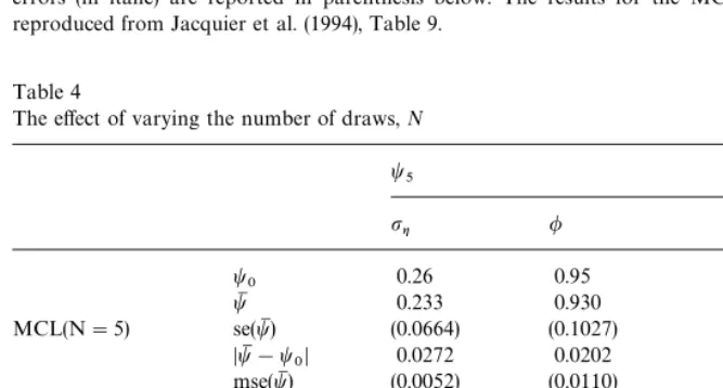
Table 4

The effect of varying the number of draws,N

t₅

0D 0.0272 0.0202 0.0456

mse(tM) (0.0052) (0.0110) (0.0022)

tM 0.256 0.936 !0.372

MCL(N"20) se(tM) (0.0583) (0.1003) (0.0126)

DtM!t

0D 0.0044 0.0142 0.0452

mse(tM) (0.0034) (0.0103) (0.0022)

tM 0.257 0.937 !0.372

MCL(N"40) se(tM) (0.0490) (0.0993) (0.0126)

DtM!t

0D 0.0029 0.0133 0.0452

mse(tM) (0.0024) (0.0100) (0.0022)

Note: This table reports the results of the simulation experiment on a single set of parameter values, t₅. Samples of length¹"_{500 of the basic SV model are simulatedK}"_{500 times and estimated by} MCL. Values 5, 20, and 40 in parenthesis behind the MCL label signify the number of draws,N, employed by taking the expectation in Eq. (5). For each estimator the average parameters estimates, the sample standard deviations, the absolute bias and the mean squared error are reported in the rows labelledtM, se(tM),DtM!t

6More detailed estimation results are reported in Table 7.

7We are grateful to Jon Danielsson for pointing out this procedure.

three parameters,/,p

ganda(i.e.pN) the comparison in terms of absolute bias and

standard deviation reveals a small improvement in accuracy when the number

of draws,Nis increased from 5 to 20. However, further increasingNto 40 leads

to negligible improvement. Since the increase in accuracy occurs in the third

decimal place for model parameters we recommend settingN"5 in empirical

applications.

These results are very encouraging. They demonstrate that the MCL estimator exhibits very satisfactory small sample performance which is directly comparable to the fully efficient Bayesian MCMC method. The evidence also suggests that these results can be achieved by using a very small number of draws.

4.2. S&P500 return series

The performance of the MCL estimator is further illustrated by fitting the model to the seasonally adjusted (Gallant et al., 1992) S & P 500 returns. JPR

and Danielsson (1994b) has already utilized a subset of the data

(2/1/80—30/12/87,¹"2,022 observations) to fit the basic SV model.

Re-estima-tion by MCL allows not only for a comparison of the point estimates but also for the comparison of the computational requirement. The results of the

estima-tion are reported in the table below:6

a / p_g Time min

MCL !0.00 0.96 0.16 1 : 21

MCMC !0.00 0.97 0.15 7 : 15

Danielsson’s MCL !0.00 0.97 0.15 10 : 45

The parameter estimates are almost identical across the three estimation

methods. The time requirement was calculated in the following manner.7First,

Danielsson’s code was executed on our machine. The algorithm required 5:59 min to converge. On the other hand, starting at the same initial value, the MCL estimation method required 0:58 min to achieve convergence. The figure of 1:21 min in the above table for MCL was obtained by calibrating it to the time requirement reported in Danielsson (1994b). These results suggest that estima-tion via the MCL method is computaestima-tionally more efficient than the MCMC and the alternative importance sampling methods.

Secondly, the basic SV model was fitted to the entire data-set

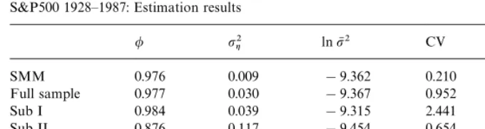
Table 5

S&P500 1928—1987: Estimation results

/ p2_g lnpN2 CV LogLik

SMM 0.976 0.009 !9.362 0.210 —

Full sample 0.977 0.030 !9.367 0.952 !34,610

Sub I 0.984 0.039 !9.315 2.441 !8,689

Sub II 0.876 0.117 !9.454 0.654 !8,799

Sub III 0.970 0.034 !9.579 0.760 !8,554

Sub IV 0.989 0.010 !9.219 0.630 !8,512

Note: This table reports the parameter estimates of the basic SV model when fitted to the adjusted daily observations on the S&P500 stock index level, 1928—87. The row labelled ‘SMM’ reproduces the estimates of Gallant et al. (1995), Table 2, row1. The correspondence to the notation of the present paper is established by: /"_a

1,p2g"_r2

w, lnpN2"_2ln(10~2_r

y). The factor 10~2 appears

because we choose to work with percentage returns. The subsequent rows report the MCL estimates for the full sample (4/1/28—31/12/87,¹"_{16 127), and four sub-samples of equal length,}¹"_4030: Sub I (4/1/28—7/7/41), Sub II (8/7/41—30/11/55), Sub III (1/12/55—7/1/72), Sub IV(10/1/72—21/12/87).

(Gallant and Tauchen, 1996). The parameter estimates are reported in Table 5. The resulting point estimates are very close to the SMM values obtained by

Gallant et al. (1995) except for the estimate of p2

g. The sub-period analysis

reported in the remainder of Table 5 illustrates that the parameter estimates,

and in particular the impliedC»are not stable across the sub-periods. This may

explain why Gallant et al. (1995) found the SV model to be incapable of capturing the time series dynamics of the S & P500 index. It is not surprising that, when a data set of roughly 60 yr of daily observations is used, some regime switches may be present.

This application also demonstrates that large data-sets present no difficulty for the estimation by MCL.

5. Further issues

Having shown that the MCL estimator exhibits satisfactory finite sample performance we would now like to turn to the practical issues in SV model estimation and indicate some of the interesting extensions of the basic SV model.

5.1. The inlier problem

Since our method, as much as QML, relies on the use of the linear state space, taking the logarithms of squared mean adjusted returns becomes a problem when zero, or small values are encountered. In particular, if the drift in of the

asset can be assumed to be zero (k

is possible that some returns will be zero. In many practical applications, however, equality of prices at two successive observations in time, leading to zero returns, arise due to data irregularities. For instance, properly accounting for holidays eliminates many ‘zero’ returns in most daily exchange rate series. Deleting such observations from the sample eliminates the inlier problem. Alternatively, the updating equations of the Kalman filter can be modified so as to handle missing values (Harvey, 1989, p. 143).

If an inlier cannot be assumed to be an irregular observation there are three alternatives of dealing with the problem. First, the sample mean of the series (or some general ARMA specification) may be subtracted from the observations. While the method may be feasible numerically (the resulting series may be devoid of entries identically equal to zero) it does not solve the problem conceptually. Secondly, Fuller (1996) suggests a transformation which mitigates the inlier problem by shifting some probability mass towards the center of the distribution:

where jis some subjectively chosen constant, e.g. 0.02, and s2_r is the sample

variance of returnsr

t. Breidt and Carriquiry (1996) show that this

transforma-tion improves the performance of the QML estimator and mitigates the inlier problem. This method, however, remains inefficient.

Finally, one may cut off the inliers by setting the observation at some valuei:

ln*(r2

t)"ln(r2

tIM_rtwiN)#lni2I_M

rt:iN (10)

where IM_>N is the indicator function, and i is a small number. Invariably, the

choice of i is subjective but it is demonstrated below that Eq. (10) leads to

reasonably good MCL estimates for very smalli.

To assess the performance of the MCL and QML methods across various

values ofiwe designed the following Monte Carlo experiment. For the

para-meter triplett

5we generated the basic SV model as before, except that the mean

equation disturbances,m

tin Eq. (1) have now a 10% chance of taking the value

zero and 90% chance of being drawn from N(0,1). It is rarely the case in practical applications that 10% of the sample are identically equal to zero but the experiment has been designed to illustrate the behavior of the estimator in extreme situations. The generated series was then transformed according to

Eq. (10) with ln(i2_i) taking the values of!20,!30, !100, and!200. The

results of the simulations for QML and MCL are presented in Table 6 and compared to those of Section 4.

It is apparent that the performance of QML leaves much to be desired. The

bias and the standard errors are very sensitive to the choice of i. As i is

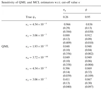
Table 6

Sensitivity of QML and MCL estimators w.r.t. cut-off valuei

p_g / a

Note: This table reports the results of the simulation experiment on a single set of parameter values, t₅. Samples of length¹"_{500 of the basic SV model with 10% zero values are generatedK}"₅₀₀ times and estimated by QML and MCL. Inliers are cutoff ati_iwhere the cutoff constantsi₁—i₄

were chosen so as to correspond to ln(_i2

i)" !20,!30,!100 and!200.

three parameters. However, the decline in precision is not homogenous across

the three model parameters. Interestingly, for smalli(e.g.i

4"3.72]10~44) the

bias in the estimate of the autoregressive parameter / disappears, while the

biases in the estimates ofa(i.e.pN) andp

gremain very large.

The results of the MCL estimator are considerably better. The bias and the

standard errors on all three model parameters decrease with the cutoff valuei.

8This is different from the Harvey et al’s (1994) QML setup where the variance of the measure-ment equation,Hin the state space formulation is treated as a parameter.

5.2. Extensions of the basic SV model (I):Heavy¹ails

The unconditional density of many financial series exhibits larger kurtosis than can be captured by simply incorporating conditional heteroscedasticity into a Gaussian process. The basic SV model can be generalized so as to allow

the mean equation disturbances,m

tin Eq. (1) to follow aStudent-tdistribution

with ldegrees of freedom. In this case the density of the transformed

distur-bances,e

verified by taking logarithms of Eq. (3a), and expanding ln(1#x) as a Taylor

series.

A suitable importance sampling density is found by equalizing density slopes as described in Section 3.1. The first derivative of the log density in Eq. (3a) is

d

1(z)"12

G

C

l#ez

DH

so that the updating equations forHI _t become

HI

t" 2eLt

eeLt[(l#1/l#eeLt)]!1 t

"1,₂,¹. (6a)

Again, the Gaussian equations (6) are obtained in the limit, as lPR in

Eq. (6a). Moreover, Eq. (6a) automatically ensures the nonnegativity of HI

t,

which can be verified by observing that the signs of the numerator and

denomin-ator are identical for any value of l and eL

t. The computation of the MCL

likelihood (5) involves the quantitiesl(e(_ti)) in Eq. (7) which are now constructed

via:

t is given by Eq. (6a) after convergence. The number of degrees of

freedom,lenters the parameter vectort, over which the likelihood function is

maximised.8

To illustrate the validity of the method, we proceed to fitting the SV-tmodel

Table 7

Estimates of the SV model with fat-tailed disturbances

/ p2_g lnpN2 l CV LogLik LR

tK 0.960 0.026 !9.313 — 0.389 !4,311.6 26.6

se(tK) (0.018) (0.009) (0.094) — — — —

tK 0.984 0.007 !9.498 7.634 0.255 !4,298.3 —

se(tK) (0.010) (0.003) (0.122) (0.003) — — —

Note: This table reports the estimation results of the SV model where the mean equation distur-bances follow aStudent-tdistribution withl degrees of freedom. The data-set consists of daily observations on the S&P500 stock index level in the period 2/1/80—30/12/87. The return series are prefiltered to remove the calendar effects as documented in Gallant et al. (1992). The sample length is ¹"_{2022 observations. The standard errors of (}/_,p2

g,l) are obtained from the numerical

approxima-tion to the Hessian, while the standard errors of the estimate of lnpN2are taken from the correspond-ing diagonal element of the state covariance matrix,P_T. The likelihood ratio test statistic follows the s₂₁distribution.

9Parameter estimates of Table 2.5 were used to draw two samples of the SV process the density of which is presented in the figure. Thet-distributed random numbers were constructed in accordance with the Bailey (1994) algorithm.

estimated number of degrees of freedom is 7.634, well in the range of empirical

estimates reported by Bollerslev (1987) using the GARCH-t model:

6.211—13.889. The likelihood ratio test statistic takes the value 26.6 which is

significant at the 1% level when compared to the relevant critical value of the

s₂₁distribution. Similarly, the standard error on lindicates the significance of

this parameter. The introduction of the Student-t distributed mean equation

disturbances reduces the value of the implied coefficient of variation,C»from

0.389 to 0.255. Intuitively, lower variance of the latent process is sufficient to account for the variability in the series.

Finally, Fig. 5 demonstrates that the unconditional density of the S & P500 returns is closely approximated by the unconditional density from the estimated

SV-tmodel.9By contrast, the unconditional density of the basic SV model (with

normal m

t) does not capture as well the unconditional distribution of asset’s

returns. Thus the MCL estimator can be easily adjusted so as to incorporate heavy tailed distributions.

5.3. Extensions of the basic SV model (III):Explanatory variables

10The data-set consists of the returns on the CRSP value-weighted US market index for the period 3/7/62—31/12/87 resulting in¹"_{6409 observations.}

variables could be intervention dummies, seasonal components, or regressors like option implied volatility, trade volume data, etc. The empirical validity of the SV model with explanatory variables has been examined elsewhere (Ghysels and Jasiak, 1996; Board et al., 1997) but it deserves to be mentioned here that the MCL method need not be modified to handle this extension. More importantly, since the explanatory variables enter the state vector (see Appendix A) the dimensionality of the optimisation problem is unchanged. For instance, the

basic SV model withkexplanatory variables requires the optimization in only

two directions,/andp

g. This is very useful since multidimensional nonlinear

optimization is a formidable task.

5.4. Extensions of the basic SV model (I»):Non-zero correlation

When the linearizing transformation—which transforms the basic SV model

into the linear state space form—is applied, information regarding the

correla-tion between the return and the (log)variance process is lost. In the context of QML estimation Harvey and Shephard (1996) shows that this information can be recovered by conditioning on the signs of the returns. The augmented model takes the form:

the correlation between the two original residuals in Eq. (1). Conditional on the

signs, the distribution of the new transition equation disturbances, gJ_t is no

longer Gaussian leading to the loss of efficiency of the MCL estimator. The effect, however, will not be large since the symmetry of this density allows the Kalman filter to match the first three moments.

No modifications to the MCL estimation procedure are required since the

filtering and smoothing algorithms—see Appendix A—are all written for the

correlated state space model. The correlation coefficient,oenters the parameter

vectort"(p

g,/,o) over which the likelihood function is optimized. Fitting the

model to the CRSP data-set10used by Nelson (1991) and Harvey and Shephard

Table 8

Estimates of the SV model with nonzero correlation

/ p2_g lnpN2 o CV LogLik LR

tK 0.988 0.018 !10.017 — 1.11 !13,680 124

se(tK) (0.003) (0.003) (0.136) — — — —

tK 0.985 0.021 !9.924 !0.375 0.99 !13,618 —

se(tK) (0.003) (0.003) (0.109) (0.004) — — —

Note: This table reports the estimation results of the SV model where the mean and variance equation disturbances are allowed to be correlated. The data-set consists of the returns on the CRSP value-weighted US market index for the period 3/7/62—31/12/87 used by Nelson (1991) and Harvey and Shephard (1996). The sample size is¹"_{6409 observations. The standard errors of (}/_,p2

g,o) are

obtained from the numerical approximation to the Hessian, while the standard errors of the estimate of lnpN2are taken from the corresponding diagonal element of the state covariance matrix,P

T. The

likelihood ratio test statistic follows thes21distribution.

error ono_L indicate the statistical significance of the correlation coefficient. The

MCL estimates are less sensitive to the presence of correlation than the QML

estimators. Omittingodoes not significantly alter the estimates of the remaining

parameters (/, p

g, pN). Furthermore, the standard errors on all parameters

estimates are smaller than the QML errors, reflecting the increased efficiency of the estimator.

6. Conclusion

In this paper, the Monte Carlo likelihood (MCL) method of estimating stochastic volatility (SV) models is implemented successfully. The represent-ation of the SV model is in a linear state space form so the Kalman filter can be employed to compute the Gaussian likelihood function via the prediction error decomposition. However, due to the log chi-square disturbances in the measurement equation of the SV model, the Gaussian likelihood will only make up a part of the true likelihood function. The MCL estimator proposed here approximates the remainder term via Monte Carlo simulation. As the

number of simulationsNincreases, the approximation becomes more accurate.

The finite sample performance of the MCL is examined in a simulation experi-ment. The results indicate full efficiency of the estimator across a range of possible parameter values even for very moderate simulation sizes such asN"5.

extensions in detail: fat-tailed distribution of the mean equation disturbances, inclusion of explanatory variables and the nonzero correlation model. The illustrations have shown that all these extensions can be handled by the MCL straightforwardly. Finally, it is noticeable that these modifications do not require any substantial changes to the methodology of MCL or any changes to the Kalman filter smoother algorithms.

Acknowledgements

We are indebted to Jim Durbin and Andrew Harvey as well as seminar participants of the ESEM 96 Conference in Istanbul for helpful comments and suggestions. The comments of the Associate Editor and an anonymous referee helped greatly improve the quality of the paper. The second author is grateful to the ESRC for financial support as part of the project ‘Interrelationships in Economic Time Series’, grant No. R000235330. All remaining errors remain our responsibility.

Appendix A.

1. The general univariate state space model (Harvey, 1989) is:

y

where y_t is a scalar observation,a_t is the (m]1) state vector, the covariance

matrices H_t (1]l) and Q_t (m]m) are nonsingular, while the measurement

and transition equation disturbances may be contemporaneously

corre-lated with an (m]1) nonzero covariance matrixG

t. In case of the SV model,

the elements (or functions of the elements) of the parameter vectort"(/,p

g,o)

enter into the appropriate elements of Q

t, ¹

t, Gt and ct. The long-run

volatility level,pN (along with any explanatory variables) enters the state vector

a_t which reduces the dimensionality of the nonlinear optimization problem

of maximizing the likelihood function with respect to the parameter vector;

see below. For instance, an correlated SV model withkexplanatory variables,

zkt grouped into z

wherec

tis (k]1),ekis a (k]1) vector of zeros,Ikis the (k]k) identity matrix,

and s

t is the sign of the return at time t. The basic SV model is obtained as

a special case by settingo"0 andk"1,z1

t"1,∀t. The Kalman filter is given by

l_t"y

the unconditional variance matrix of the state vector which may contain diffuse

elements. The parameter estimates fortare obtained by numerically optimizing

the Gaussian log likelihood function as given by

ln¸

The estimate of lnpN2is given by the relevant element ofa_t while the standard

errors are obtained from the relevant diagonal elements ofP_t(Harvey, 1989, p.

367).

2. The Kalman smoother (de Jong, 1988; Koopman, 1993) is used to con-struct:

where y is the vector of all observations, J_t"H

tK@tNtGt, and the remaining

quantities are obtained from the backwards recursions:

e

T"0. The prediction errors, l

t, their

variances, F

t, and the Kalman gain matrix, Kt are outputs of the Kalman

filter.

3. A special version of de Jong and Shephard’s (1995) simulation smoother is

where the quantitiese_J

required, the Kalman filter and the recursions forDI

t,Mt,CI t,NI t~1need only be

applied once since these quantities remain the same for each sample.

References

Andersen, T.G., 1994. Stochastic autoregressive volatility: a framework for volatility modeling. Mathematical Finance 4, 75—102.

Andersen, T.G., S+rensen, B., 1996. GMM estimation of a stochastic volatility model: a Monte Carlo Study. Journal of Business and Economic Statistics 14, 328—352.

Bailey, R.W., 1994. Polar generation of random variates with thet-distribution. Mathematics of Computation 62, 779—781.

Baillie, R.T., Bollerslev, T., 1989. The message in daily exchange rates: a conditional variance tale. Journal of Business and Economic Statistics 7, 297—305.

Bera, A.K., Higgins, M.L., 1993. ARCH models: properties, estimation and testing. Journal of Economic Surveys 7, 305—366.

Board, J.L.G., Sandmann, G., Sutcliffe, C.M.S., 1997. The effect of contemporaneous futures market volume on spot market volatility. mimeo, London School of Economics.

Bollerslev, T., 1987. A conditional heteroskedastic time series model for speculative prices and rates of return. Review of Economics and Statistics 69, 542—547.

Bollerslev, T., Chow, R.Y., Kroner, K.F., 1992. ARCH modelling in finance: a review of the theory and empirical evidence. Journal of Econometrics 52, 5—59.

Bollerslev, T., Engle, R.F., Nelson, D.B., 1993. ARCH models. In: Engle, R.F., McFadden, D.L. (Eds.), Handbook of Econometrics, vol. IV, Noth-Holland, Amsterdam.

Breidt, F.J., Carriquiry, A.L., 1996. Improved quasi-maximum likelihood estimation for stochastic volatility models. In: Zellner, A., Lee, J.S. (Eds.), Modelling and Prediction: Honouring Seymour Geisel. Springer, New York.

Danielsson, J., 1994b. Comment on Jacquier, Polson and Rossi. Journal of Business and Economic Statistics 12, 389—392.

de Jong, P., 1988. A cross-validation filter for time series models. Biometrika 75, 594—600. de Jong, P., Shephard, N., 1995. The simulation smoother for time series models. Biometrika 82,

339—350.

Durbin, J., Koopman, S.J., 1997. Monte Carlo maximum likelihood estimation for non-Gaussian state space models. Biometrika, 84, 669—684.

Durbin, J., Koopman, S.J., 1998. Time series analysis for non-Gaussian observations based on state space models. mimeo, London School of Economics.

Fridman, M., Harris, L., 1996. A maximum likelihood approach for non-Gaussian stochastic volatility models. mimeo, University of Southern California.

Fuller, W.A., 1996. Introduction to statistical time series. 2nd Ed., Wiley, New York.

Gallant, A.R., Hsieh, D., Tauchen, G., 1995. Estimation of stochastic volatility models with diagnostics. mimeo, Duke University.

Gallant, A.R., Rossi, P.E., Tauchen, G., 1992. Stock prices and volume. Review of Financial Studies 5, 199—242.

Gallant, A.R., Tauchen, G., 1996. Which moments to match. Econometric Theory, forthcoming. Ghysels, E., Harvey, A.C., Renault, E., 1996. Stochastic volatility. In: Rao, C.R., Maddala, G.S.

(Eds.), Statistical Methods in Finance. North-Holland, Amsterdam.

Ghysels, E., Jasiak, J., 1996. Stochastic volatility and time deformation: an application to trading volume and leverage effects. mimeo, Univerite´ de Montre´al.

Harvey, A.C., 1989. Forecasting, structural time series models and the kalman filter. Cambridge University Press, Cambridge.

Harvey, A.C., Shephard, N., 1993. Estimation and testing of stochastic variance models. mimeo, London School of Economics.

Harvey, A.C., Shephard, N., 1996. Estimation of an asymmetric stochastic volatility model for asset returns. Journal of Business and Economic Statistics 14, 429—434.

Harvey, A.C., Ruiz, E., Shephard, N., 1994. Multivariate stochastic variance models. Review of Economic Studies 61, 247—264.

Hull, J., White, A., 1987. The pricing of options on assets with stochastic volatilities. Journal of Finance 42, 281—300.

Jacquier, E., Polson, N.G., Rossi, P.E., 1994. Bayesian analysis of stochastic volatility models. Journal of Business and Economic Statistics 12, 371-417 (with discussion)

Jacquier, E., Polson, N.G., Rossi, P.E., 1995. Stochastic volatility: univariate and multivariate extensions, R.L. White Centre for Financial Research, DPd19-95. Wharton School, University of Pennsylvania.

Kim, S., Shephard, N., Chib, S., 1996. Stochastic volatility: likelihood inference and comparison with ARCH models. mimeo. Nuffield College, Oxford.

Kitagawa, G., 1987. Non-Gaussian state space modelling of nonstationary time series. Journal of the American Statistical Association 82, 1032-63 (with discussion).

Koopman, S.J., 1993. Disturbance smoother for state space models. Biometrika 80, 117—126. Lamoureux, C.G., Lastrapes, W.D., 1990. Heteroskedasticity in stock return data: volume versus

GARCH effects. Journal of Finance 45, 221—229.

Lamoureux, C.G., Lastrapes, W.D., 1993. Forecasting stock-Return variance: toward an under-standing of stochastic implied volatilities. Review of Financial Studies 6, 293—326.

Melino, A., Turnbull, S.M., 1990. Pricing foreign currency options with stochastic volatility. Journal of Econometrics 45, 239—265.

Nelson, D.B., 1991. Conditional heteroskedasticity in asset returns: a new approach. Econometrica 59, 347—370.

Shephard, N., 1996. Statistical aspects of ARCH and stochastic Volatility. In: Cox, D.R., Hinkley, D.V., Barndorff-Nielsen, O.E. (Eds.), Time Series Models. Chapman and Hall, London. Shephard, N., Pitt, M.K., 1997. Likelihood analysis of non-Gaussian parameter-driven models.

Biometrika, 84, 653—667.

Taylor, S.J., 1986. Modelling Financial Time Series. Wiley, Chichester.