Regularizing Mono- and Bi-Word Models for Word Alignment
Thomas Schoenemann
Lund University, Sweden
Abstract
Conditional probabilistic models for word alignment are popular due to the elegant way of handling them in the training stage. However, they have weaknesses such as garbage collection and scale poorly be-yond single word based models (DeNero et al., 2006): not all parameters should ac-tually be used.
To alleviate the problem, in this paper we explore regularity terms that penalize the used parameters. They share the advan-tages of the standard training in that itera-tive schemes decompose over the sentence pairs. We explore the models IBM-1 and HMM, then generalize to models we term
Bi-word models, where each target word can be aligned to up totwosource words. We give two optimization strategies for the arising tasks, using EM and projected gra-dient descent. While both are well-known, to our knowledge they have never been compared experimentally for the task of word alignment. As a side-effect, we show that, against common belief, for paramet-ric HMMs the M-step isnotsolved by re-normalizing expectations.
We demonstrate that the regularity terms improve on the f-measures of the standard HMMs and that they improve translation quality.
1 Introduction
State-of-the art approaches for word alignment are based on probabilistic models. They can be split into joint models (Melamed, 2000; Marcu and Wong, 2002) and conditional models (Brown et al., 1993; Vogel et al., 1996; Wang and Waibel, 1998; Toutanova et al., 2002; Sumita et al., 2004;
Deng and Byrne, 2005; Fraser and Marcu, 2007a). While in early works the underlying basic entity was a single word, today’s advanced approaches build on sequences of words, calledphrases.
For joint models the advanced models are stand-alone approaches (Marcu and Wong, 2002). How-ever, these models are computationally hard to handle, which frequently results in maximum ap-proximations being made. This is different for the conditional models, which are easier to handle but where most approaches are based on initializ-ing from sinitializ-ingle-word based models (Brown et al., 1993; Vogel et al., 1996; Al-Onaizan et al., 1999). However, the recent work of Mauser et al. (2009) deals with pairs of source words and is trained without considering single word based models.
In this paper we much generalize on this work, considering a class of models we term Bi-word models. We consider a variant of (Mauser et al., 2009) which we call Bi-1, then proceed to derive a Bi-HMM. Our main focus is however on regu-larizing such models. We first address known con-ditional models calledsingle-word based models, focusing on a weakness known asgarbage collec-tion. We show that this weakness can be alleviated by adding an entry to every dictionary distribution as well as adding a regularity term (a weightedL1
norm). Afterwards we generalize this idea to Bi-word models. The regularity term will now be-come crucial since the garbage problem is known to worsen for conditional models that generalize single-word based ones (DeNero et al., 2006).
We cast all this as compact objective functions subject to simplex constraints, and show two ways to optimize these: via EM and via projected gra-dient descent (Bertsekas, 1999, chap. 2.1). Since each iteration decomposes over the sentence pairs, the approach is efficient and scalable. In contrast to our recent work (Schoenemann, 2011) (where we used anL0-norm) we do not use the maximum
approximation and also address Bi-word models.
Related Work on Word Alignment For a sys-tematic comparison of the most commonly used models see (Och and Ney, 2003). Apart from the classical approaches, a few other lines of work have been pursued. Indeed, for single word based models regularity terms have been considered be-fore, in particular in our recent work on the L0
-norm (Schoenemann, 2011). Otherwise most of the work has focused on combining asymmetric conditional approaches. Zens et al. (2004) inter-twine the training of both directions by exchang-ing information in-between the iterations. Liang et al. (2006) propose to include the products of the conditional marginals for each training direc-tion into the objective funcdirec-tion. Grac¸a et al. (2010) postulate that the posterior marginals for both di-rections be equal. They also propose an asymmet-ric variant that favors 1-to-1 alignments. The idea of posterior regularization has further been pur-sued in the machine learning community (Mann and McCallum, 2007).
We further note the approaches (Matusov et al., 2004; Taskar et al., 2005; Lacoste-Julien et al., 2006) that focus on the computation of alignments given symmetrized cost. Some of them also in-clude novel ways to train the models.
Finally, our EM-scheme bears resemblance to the works (Berg-Kirkpatrick et al., 2010; Ganchev et al., 2010), but we address substantially different models.
2 Mono-Word Models
In this section we review the employed single word based models. We call them Mono-word models as we find the term more handy, in par-ticular when it comes to distinguishing them from the pair-based models in the next section.
All discussed models formalize the (condi-tional) probability that a given English sentence
e=eI1, consisting ofI words, produces a foreign
sentence f = fJ
1 withJ words. This probability
is denotedp(f|e). We will refer toeas the source
sentence and tof as the target sentence. The
con-sidered models are all based on hidden variables calledalignments. For Mono-word models the as-sumption is that each target word is aligned to at most one source position. The aligned position of target wordjis denotedaj ∈ {0, . . . , I}, where0 indicates unaligned words. The alignment of the entire sentence pair is denoted a = aJ
1 and the
probability is modeled as
p(f|e) =X
a
p(f,a|e) .
The models differ in how this new joint probability is modeled, but they all factor it as
p(f,a|e) =Y j
p(fj|eaj)·p(aj|aj−1, j, I) .
For the first term (dictionary probability) all mod-els use the same non-parametric representation. For the second term (alignment probability) they differ. The IBM-1 simply setsp(aj|aj−1, j, I) =
1/(I + 1), resulting in a convex model. We also consider the non-convex HMM, which mod-elsp(aj|aj−1, I), getting rid of the dependence on j. To avoid overfitting a parametric model is used, based on considering the differenceaj−aj−1.
De-tails are given in the next section.
3 Bi-Word Models
In this paper we consider a more general class of conditional models, which we call Bi-word mod-els. Here we are much generalizing on the work of (Mauser et al., 2009).
Now each target word is allowed to align to up to two source words. The alignment of tar-get word j is expressed as the tuple (aj,1, aj,2),
where the allowed set of values is a subset of
{0, . . . , I} × {0, . . . , I}. The value(0,0)will de-note unaligned words. In any other case we require thataj,2 > aj,1. Ifaj,1 is 0 the word is aligned
only once. Ifaj,1 >0it is aligned twice. We
fur-ther forbid the case whereaj,1 > 0andaj,2 = I
since at the sentence end the considered data usu-ally contain a punctuation mark which aligns only once. Note that otherwise there are no restrictions, in particular we do not require that the two aligned words are at consecutive positions (although such knowledge could be enforced in our framework).
In the generative story of the models we first take a decision of whether the alignment of po-sition j is a double alignment or not. We
de-note this by a binary variablebj ∈ {0,1}, where a value of 1 denotes a Bi-alignment. Obviously
bj = 0impliesaj,1 = 0. Afterwards we decide on
the aligned positions and the identity of the target word:
p(f,a|e) = Y j
p(fj|eaj,1, eaj,2)·p(bj) (1)
Note that compared to the Mono-word models we have now many more dictionary parameters, as well as much more probability mass to spread. Moreover, eaj,1 and eaj,2 can be the empty word N U LL.
In this work we consider two models that gen-eralize the IBM-1 and the HMM to the new set of alignments. We call them Bi-1 (a variant of Mauser et al.’s model) and Bi-HMM, and again they differ only in the alignment probabilities. The valuesp(bj= 0)andp(bj= 1)are chosen indepen-dently ofjand fixed to0.1and0.9in this work.
The Bi-1 is a convex model and treats non-Bi-alignments as p(0, aj,2|bj = 0, I) = 1/(I + 1), just like the IBM-1. For Bi-alignments it sets p(aj,1, aj,2|bj = 1, I) = 1/K, where K is the number of possible Bi-alignments (and where
aj,1, aj,2 is an allowed constellation). Note the
(subtle) difference to the work of Mauser et al.: this work did not consider the variablesbj, so for long sentences the pairwise alignments become dominant. Further, for our models the word order matters, i.e. generallyp(f|e1, e2)6=p(f|e2, e1).
The proposed Bi-HMM factors the alignment probability in a manner similar to the Mono-HMM. First of all, for a given alignment we in-troduce the notion of the head of target position
j, denotedhj. In case the position was aligned at least once, we definehj as the smallest target po-sition aligned to j, i.e.hj =aj,1 ifaj,1 6= 0 and hj =aj,2 else. In case of unaligned positionshj is set to the head of the largest aligned previous target position. Hence we use a full first-order de-pendence, which in practice requires doubling the state space - see (Vogel et al., 1996). The align-ment probabilities are now
p(0, aj,2|hj−1, b= 0, I) = pinter(aj,2|hj−1, I)
and foraj,1 >0
p(aj,1, aj,2|hj−1, b= 1, I) =pinter(aj,1|hj−1, I) ·pintra(aj,2|aj,1).
Note that both cases rely on the same probabil-ity modelpinter(·|·). The second case has an ad-ditional distribution pintra(·|·). Both are mod-eled separately using a parametric distribution de-scribed below. Note thatpintra(i|i0) = 0ifi≤i0.
Superficially the Bi-HMM looks similar to (Deng and Byrne, 2005). However, this latter is actually a Mono-word model.
Parametric HMMs. It is well-known that HMMs for word alignment perform best using parametric alignment probabilities. For both the Mono-HMM and the Bi-HMM, we follow Vogel et al. (1996) and consider only the differencei−i0
to modelpinter(i|i0, I). Here, only differences be-tween−5and5are modeled by separate parame-tersr−5, . . . , r5, all larger differences are captured
by a single parameterrL. To make this a probabil-ity distribution, the latter parameter is spread uni-formly over all possible differences (with absolute larger than 5) in the respective context. Lastly, we introduce parametersp0andp1(p0+p1= 1), where p0 denotes the probability for unaligned words.
The alignment probability is now
pinter(i|i0, I) =
p0 ifi= 0
p1rτii−0,Ii0 ifi >0, |i−i0| ≤5 p1·rL
τi0,I|{i00:|i00−i0|>5}| else,
with1
τi0,I =
X
1≤i≤I:|i−i0|≤5
ri−i0+rL . (2)
A special case arises for the initial alignment prob-abilities p(h1=i|I). Rather than fixing them to
1/(2I) (including empty words), as is common, we model these parametrically (with renormaliza-tion, but without grouping).
In case of the Bi-HMM, there is further the probabilitypintra(·|·), which we also parameterize based on positive distances, grouping those larger than 5. In principle, each of the three arising dis-tributions has its own parameter set. However, the initial probability and the inter-alignment model share the parametersp0andp1.
4 Objective Functions
In word alignment one is given a large set of sen-tence pairs, not a single pair. We denote the sth
pair by fs,es. The standard approach to word
alignment is maximum likelihood, i.e. minimiz-ing
−X
s
log(p(fs|es))
over the parameters of the model. Here, we are considering a conditional model, which can be any of the above mentioned.
1If differences of more than5are impossible, the termr
L
Such models are known to have weaknesses calledgarbage collection. This refers to the phe-nomenon that rarely occurring source words tend to align to a significant portion of the target words in the respective sentences, since the probability mass of the frequent words is better used to ex-plain the sentences without rare words. The effect is known to worsen when one moves beyond sin-gle word based models (DeNero et al., 2006).
It is known that joint models suffer less from this deficiency when dealing with the same set of possible alignments. However, joint models are usually hard to handle computationally, whereas the mentioned conditional models behave quite nicely. Hence, we use conditional models, but pro-pose to alter the training criterion. We add a regu-larity term that penalizes the used probability mass in a (non-negative) weightedL1manner. We state
this for Bi-word models, but note that the Mono-word models are included by fixinge1=N U LL:
−X
s
log(p(fs|es)) +X
e1,e2,f
wfe1,e2p(f|e1, e2) (3)
Herewe1,e2 ≥ 0are known weights (see below).
For the new objective to make sense, we need to augment the parameter space: for every constella-tione1, e2, we add a probabilityp(N U LL|e1, e2). In the standard ML-criterion this entry will always be set to0. Not so with our new criterion: since we set the respective weighting factorwN U LLe1,e2 to
0it may be cheaper not to use the entire mass to explain the corpus.
Choice of Weights. When dealing with Mono-word models we only penalize rare Mono-words since they cause the garbage collection phenomenon. LetN(e)be the number of times the source word
eoccurs in the corpus. If N(e) ≥ 6we setw∗0,e
to0, otherwise it is set toλ[6−N(e)], whereλis
some weight. We foundλ= 2.5to work well. For Bi-word models we presently set all Mono-word weights w0∗,∗ to 0. The Bi-word penalties are based on a value ofλ = 0.5, but rare source word pairs pay a larger penalty (The equation is
λ·max{1,5−N(e1, e2)}, whereN(e1, e2)is the number of times the paire1, e2occurred).
5 Optimization Strategies
We present two optimization schemes to handle the arising minimization problems: one is based on Expectation Maximization (EM), the other on projected gradient descent (PGD). To make the
paper self-contained, we include a sketch of the relevant equations, noting that they are probably known in other contexts. We detail the scheme on the Bi-word models, the Mono-word models can be handled analogously.
Constraints First of all we note that we are dealing with aconstrainedoptimization problem, since the objective (3) is minimized over the pa-rameters of probability distributions. For the dic-tionary parameters we have positivity constraints and normalization constraints:
p(f|e1, e2)≥0 ∀f, e1, e2 ,
X
f
p(f|e1, e2) = 1 ∀e1, e2 .
This is known as a product of simplices, a rela-tively easy constraint system. For the Bi-1 there are no more parameters to optimize.
For the Bi-HMM (and also the Mono-HMM) there are the parametersr−5, . . . r5 andrL of the inter-alignment model. Each one comes with a positivity constraint. Moreover, these parame-ters are determined only up to scale, so we in-troduce the simplex constraint that they sum to1: P5
k=−5rk+rL = 1. The same principle applies to the parameters of the initial probability and of
pintra(·|·).
5.1 Projected Gradient Descent
We first present a solution based onprojected gra-dient descent (PGD) (Bertsekas, 1999, chap. 2), which is applicable since our constraint set is con-vex. Even though EM is usually the better suited method, we recommend reading this section as some auxiliary problems of EM are optimized by a very similar method.
Obviously, the gradient of the regularity term (w.r.t. the dictionary parameters) is the weight vector with entrieswfe1,e2. Further, the gradient of
the standard maximum likelihood term is additive over the sentences. Hence, in the following we only state the gradients of a single sentence pair, i.e. ∂
∂θ −log(p(fs|es)), whereθis either a dictio-nary or an alignment parameter.
All considered models are so-called multino-mialdistributions. As shown in the appendix, for such distributions the gradient w.r.t. the dictionary parameters is given by
∂
considered sentence pair. Note that the numera-tor of the ratio is theexpectationoff aligning to
e1ande2 in the given sentence pair. This
expres-sion is also a fundamental building block of stan-dard EM. For the Mono-1 and Bi-1 this is simply a sum over the source positionsj. For the
Mono-and Bi-HMM it can be calculated by the forward-backward algorithm (Baum et al., 1970).
With a similar argument one can derive the par-tial derivatives of the alignment parameters. We exemplarily detail this forpinter. Letθdenote any of the parametersp0, p1, r−5, . . . , r5andrL. Then one can show that
∂ source word is aligned to positioniwhen the head
of the previous source word wasi0.
It remains to derive the partial derivatives of
p(i|i0, Is)w.r.t. the alignment parameters. Forp0
andp1 this is straightforward. For a regular count rkwith|k| ≤5we have
A very commonly used method for word align-ment isexpectation maximization(Neal and Hin-ton, 1998). We give a modified version that han-dles our new objective function. Note that mod-ifications of EM have been derived before, e.g. (Ganchev et al., 2010).
Traditionally, EM is used for standard maxi-mum likelihood optimization. Denoting the pa-rameters of the model as θ, the respective
mini-mization problem would be
min
The function to be minimized is called negative log-likelihood. It follows from (Neal and Hinton, 1998) that the function
F(θ,θ˜) =
is an upper bound on the negative log-likelihood function, independent of the choice ofθ˜. In fact, F(θ,θ)is exactly the negative log-likelihood for
θ. As a consequence,
upper bounds our new objective (3) - note that all p(f|e1, e2) are entries in the vector θ. As in
standard EM, we now perform coordinate descent on this new function: we iteratively update θ˜to
the vector that minimizes the objective for fixed
θ. The optimal value is given as the expectation
of alignments given θ (Neal and Hinton, 1998),
which is why this term is generally called E-step. The respective calculations in our case are exactly as the ones performed in gradient descent.
for the given θ˜ and hence the given coefficients p(as|fs,es,θ˜). While for simple models there is often an analytic solution, in our case we are not aware of one foranyof the parameters (except for special cases, e.g. when allwef1,e2 are 0). Note,
that this implies that the popular toolkit GIZA++ is not doing the M-step correctly: when apply-ing the equations derived below, we verified that renormalizing expectations doesnotminimize the M-step energy. Moreover, with the common pro-cedure the total energy usually only decreases in the first few iterations, after that it often increases. The arising M-step decomposes into several in-dependent optimization problems. In particular, there is a separate problem for eache1, e2 to
up-date the respective dictionary distribution. The function to be minimized is
X
f
wfe1,e2p(f|e1, e2)−cfe1,e2log(p(f|e1, e2)) ,
where the weightscf,e1,e2are the expectations
(un-der the previousθ) offaligning toe1ande2. We
solve this via gradient descent with the gradient
∂
In special cases more efficient schemes are ap-plicable. In particular it is well-known that if
wfe1,e2 = 0 for allf the optimal solution is given
by re-normalizing the coefficientscfe1,e2. Ifw f e1,e2
is constant for all f 6= N U LL, then in prin-ciple one only has to determine the probability
p(N U LL|e1, e2). The remaining mass can again
be spread according to normalized coefficients. For the alignment parameters, we again only discuss pinter(·|·), where the auxiliary energy is
X
and the gradient for an alignment parameterθ
∂
The inner derivatives were given in section 5.1. The parametersp0 andp1 are very simple to
de-rive.
6 Experiments
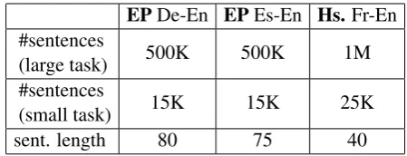
We report results on three different data sets, in both directions each. The first two are Europarl sets (in the original casing), where we consider
EPDe-En EPEs-En Hs.Fr-En
#sentences
(large task) 500K 500K 1M
#sentences
(small task) 15K 15K 25K
sent. length 80 75 40
Table 1: Statistics of the considered tasks. Es = Spanish, De = German, Fr = French, En = English, Hs. = Canadian Hansards, EP = Europarl. “K” denotes a thousand, “M” a million.
English-German2 and English-Spanish3. Further, we consider the well-known Canadian Hansards task (French-English, lowercased). In all cases we report weighted f-measures (Fraser and Marcu, 2007b) on the publicly available gold alignments. We use a weighting factor ofα = 0.1, which per-formed well in Fraser and Marcu’s work.
For the Mono-word models we consider large scale tasks with at least500000sentence pairs. For the Bi-word models the demand on computational resources is much higher, so we use tasks with 15000to25000sentence pairs. We also evaluate the Mono-word models here, showing that the reg-ularity term becomes more important in the case of scarce training data.
The most important statistics of all tasks are listed in Table 1. The methods required no more than 4 GB memory on these tasks. The running times on the large scale tasks sometimes slightly exceeded a day. For the small scale tasks even the Bi-word models need less than12hours. Without regularity, EM is clearly faster. But with regularity terms, EM and PGD are roughly equal in speed. In general, PGD finds a slightly higher energy than EM.
6.1 Comparison of Models
In this paper we have introduced new objective functions and argued that they alleviate some of the deficiencies of standard maximum likelihood for conditional models. As a consequence, we are interested in comparing models and objective functions, and not so much in getting the last bit of practical performance (f-measure).
Hence, when comparing4 to GIZA++ we turn
2Gold alignments available at
http://www.maths.lth.se/matematiklth/ personal/tosch/download.html.
3Gold alignments from (Lambert et al., 2005).
EUParl Es-En 500K EUParl De-En 500K CHans Fr-En 1M Es|En En|Es De|En En|De Fr|En En|Fr
IBM-1, EM, no reg. 64.0 64.6 68.5 71.5 82.7 83.3
IBM-1, EM, with reg. 64.5 64.9 68.6 72.0 83.1 83.5
IBM-1, PGD, no reg. 63.5 63.6 67.0 71.0 82.6 82.3
IBM-1, PGD, with reg. 63.8 64.1 66.9 71.8 83.3 81.8
HMM, EM (GIZA++) 75.0 74.2 72.5 75.3 91.4 90.8
HMM, EM (our), no reg. 77.4 76.1 73.2 77.8 89.6 90.3
HMM, EM (our), with reg. 77.7 76.3 73.1 78.2 90.3 90.6
HMM, PGD, no reg. 75.3 73.5 70.9 75.3 89.2 88.8
HMM, PGD, with reg. 74.9 73.8 72.2 75.7 89.3 88.7
IBM-4 (GIZA++) 79.6 80.0 76.8 80.5 92.3 93.2
Table 2: F-measures (×100) for the large-scale tasks.
off smoothing. Also, we run more iterations than usual: for all methods (GIZA++, EM, PGD) we run 30 iterations of IBM-1, followed by 50 for the HMM. Here we use the same regularity terms for both models. For reference, we also evaluate the IBM-4 as implemented in GIZA++ (starting from the 50 HMM iterations, then doing 5 iterations of IBM-3 and 5 iterations of IBM-4).
For the Bi-word models we initialize the non-convex Bi-HMM by running the Bi-1 first (with the same regularity term, if any). The number of iterations is the same as for the respective Mono-word models.
Large Scale Tasks. In Table 2 we show the resulting f-measures on the large scale tasks for all mentioned strategies, including GIZA++’s HMM and IBM-4. Often our HMM outperforms GIZA++ (without smoothing), which may be due to the more precise M-step. Moreover, the regu-larity terms usually improve the results, where the effect is generally stronger the higher inflected the source language is. Still, the IBM-4 performs best everywhere, so in future work we will transfer our new objective to this model.
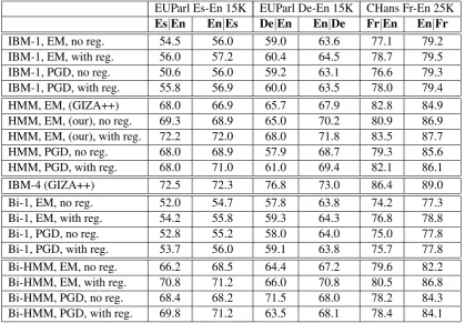
Small Scale Tasks. The results for the small tasks are given in Table 3. Here it can be seen that adding the regularity to the Mono-word mod-els greatly improves on the f-measures of the base-line HMM and sometimes gets close to the IBM-4. For the Bi-word models the regularity terms also help greatly, and in the majority of cases beat the baseline Mono-HMM (without regularity).
Like for the large scale tasks, EM performs
bet-with the new objective function we also get better results for less iterations. A systematic comparison of this is left for future work.
Method BLEU TER
our HMM, no reg. 27.94 56.98
our HMM, with reg. 28.33 56.20
GIZA++, HMM 28.04 56.83
GIZA++, IBM-4 28.71 56.15
Table 4: Evaluation of the translation quality for the large scale German→English task.
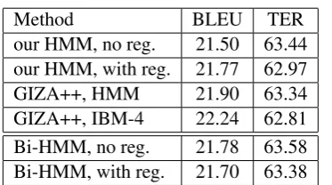
Method BLEU TER
our HMM, no reg. 21.50 63.44
our HMM, with reg. 21.77 62.97
GIZA++, HMM 21.90 63.34
GIZA++, IBM-4 22.24 62.81
Bi-HMM, no reg. 21.78 63.58
Bi-HMM, with reg. 21.70 63.38
Table 5: Evaluation of the translation quality for the small scale German→English task.
ter than PGD and the corrected M-steps often beat GIZA++.
6.2 Effect on Phrase-based Translation We give a first evaluation of the effect of our align-ments on phrase-based translation, where we ran MOSES with a 5-gram language model. We ran-domly picked translation from German to English with 750 unseen development and 3000 unseen test sentences.
As shown in the tables 4 and 5 the regularity terms do improve translation for Mono-word mod-els. The Bi-word models are presently not com-petetive. Here we are showing the BLEU accuracy measure and the Translation Edit Rate (TER).
7 Conclusion
EUParl Es-En 15K EUParl De-En 15K CHans Fr-En 25K Es|En En|Es De|En En|De Fr|En En|Fr
IBM-1, EM, no reg. 54.5 56.0 59.0 63.6 77.1 79.2
IBM-1, EM, with reg. 56.0 57.2 60.4 64.5 78.7 79.5
IBM-1, PGD, no reg. 50.6 56.0 59.2 63.1 76.6 79.3
IBM-1, PGD, with reg. 55.8 56.9 60.0 63.5 78.0 79.4
HMM, EM, (GIZA++) 68.0 66.9 65.7 67.9 82.8 84.9
HMM, EM, (our), no reg. 69.3 68.9 65.0 70.2 80.9 86.9
HMM, EM, (our), with reg. 72.2 72.0 68.0 71.8 83.5 87.7
HMM, PGD, no reg. 68.0 68.9 57.9 68.7 79.3 85.6
HMM, PGD, with reg. 68.0 71.0 61.0 69.4 82.1 86.1
IBM-4 (GIZA++) 72.5 72.3 76.8 73.0 86.4 89.0
Bi-1, EM, no reg. 52.0 54.7 57.8 63.8 74.2 77.3
Bi-1, EM, with reg. 54.2 55.8 59.3 64.3 76.8 78.8
Bi-1, PGD, no reg. 52.8 55.2 58.0 64.0 75.0 77.8
Bi-1, PGD, with reg. 53.7 56.0 59.1 63.8 75.7 77.8
Bi-HMM, EM, no reg. 66.2 68.5 64.4 67.2 79.6 82.2
Bi-HMM, EM, with reg. 70.8 71.2 66.0 70.8 80.5 86.8
Bi-HMM, PGD, no reg. 68.4 68.2 71.5 68.0 78.2 84.3
Bi-HMM, PGD, with reg. 69.8 71.2 63.5 68.1 78.4 84.1
Table 3: Resulting F-measures (×100) for the small scale tasks.
used to explain the data. We have argued that these terms reduce overfitting and demonstrated experimentally that the introduced objectives im-prove the f-measures of the generated alignments. We often beat the baseline HMM, and transferring our objective to the IBM-4 would probably beat a baseline IBM-4.
Our comparison of projected gradient descent (PGD) and expectation maximization (EM) re-vealed that EM leads to better alignments, al-though PGD finds a comparable but slightly higher objective value. We also showed that parametric HMMs induce non-trivial M-steps.
In future work we want to address IBM-3 and IBM-4 and explore the effect on phrase-based translation in greater detail.
To facilitate further research in this area, the source code associated to this work is in-tegrated into a tool called RegAligner, pub-licly available at the author’s homepage and at https://github.com/Thomas1205/RegAligner.
Acknowledgments The author thanks Ben Taskar and Jo˜ao Grac¸a for helpful discussions, as well as Alexander Engau and UC Denver for helping out with computational resources after the author had left Lund University. This work was in large part funded by the European Research Council (GlobalVision grant no. 209480).
Appendix
We now derive the partial derivative of the negative log-likelihood of a general (multino-mial) probability w.r.t. a dictionary parameter
p(f|e1, e2). This derivation is probably not novel,
but included here for completeness. The partial derivative is given by
∂
∂p(f|e1, e2) −
log(p(fs|es)) =
−p(fs1 |es) ·
" X
as
∂ ∂p(f|e1, e2)
p(fs,as|es) #
.
Now take a fixeda, and denoteka∈N0the
num-ber of times the factor p(f|e1, e2) is used in its probability, i.e.
p(fs,a|es) =ca·p(f|e1, e2)ka ,
wherecais constant w.r.t.p(f|e1, e2). Clearly ∂p(fs,a|es)
∂p(f|e1, e2)
= ca·ka·p(f|e1, e2)ka−1
= ka
p(fs,a|es)
p(f|e1, e2) .
This is how the claimed formula arises, i.e. the entire derivative is
−
P
a
kap(a|fs,es)
References
Y. Al-Onaizan, J. Curin, M. Jahr, K. Knight, J. Laf-ferty, I. D. Melamed, F. J. Och, D. Purdy, N. A. Smith, and D. Yarowsky. 1999. Statistical ma-chine translation, Final report, JHU workshop.
http://www.clsp.jhu.edu/ws99/.
L.E. Baum, T. Petrie, G. Soules, and N. Weiss. 1970. A maximization technique occuring in the statistical analysis of probabilistic functions of markov chains.
Annals of Mathematical Statistics, 41(1):164–171.
T. Berg-Kirkpatrick, A. Bouchard-Cˆot´e, J. DeNero, and D. Klein. 2010. Painless unsupervised learning with features. InConference of the North American Chapter of the Association for Computational Lin-guistisc (NAACL), Los Angeles, California, June.
D.P. Bertsekas. 1999. Nonlinear Programming, 2nd edition. Athena Scientific.
P.F. Brown, S.A. Della Pietra, V.J. Della Pietra, and R.L. Mercer. 1993. The mathematics of statistical machine translation: Parameter estimation. Compu-tational Linguistics, 19(2):263–311, June.
J. DeNero, D. Gillick, J. Zhang, and D. Klein. 2006. Why generative phrase models underperform sur-face heuristics. InStatMT ’06: Proceedings of the Workshop on Statistical Machine Translation, pages 31–38, Morristown, NJ, USA, June.
Y. Deng and W. Byrne. 2005. HMM word and phrase alignment for statistical machine translation. In
HLT-EMNLP, Vancouver, Canada, October.
A. Fraser and D. Marcu. 2007a. Getting the structure right for word alignment: LEAF. InConference on Empirical Methods in Natural Language Processing (EMNLP), Prague, Czech Republic, June.
A. Fraser and D. Marcu. 2007b. Measuring word alignment quality for statistical machine translation.
Computational Linguistics, 33(3):293–303, Septem-ber.
K. Ganchev, J. Grac¸a, J. Gillenwater, and B. Taskar. 2010. Posterior regularization for structured latent variable models. Journal of Machine Learning Re-search, 11:2001–2049, July.
J. Grac¸a, K. Ganchev, and B. Taskar. 2010. Learning tractable word alignment models with complex con-straints. Computational Linguistics, 36, September.
S. Lacoste-Julien, B. Taskar, D. Klein, and M. Jordan. 2006. Word alignment via quadratic assignment. In Human Language Technology Conference of the North American Chapter of the Association of Com-putational Linguistics, New York, New York, June.
P. Lambert, A.D. Gispert, R. Banchs, and J.B. Marino. 2005. Guidelines for word alignment evaluation and manual alignment. Language Resources and Evalu-ation, 39(4):267–285.
P. Liang, B. Taskar, and D. Klein. 2006. Alignment by agreement. InHuman Language Technology Con-ference of the North American Chapter of the As-sociation of Computational Linguistics, New York, New York, June.
G.S. Mann and A. McCallum. 2007. Simple, robust, scalable semi-supervised learning via Expectation Regularization. InInternational Conference on Ma-chine Learning, Corvallis, Oregon.
D. Marcu and W. Wong. 2002. A phrase-based, joint probability model for statistical machine trans-lation. InConference on Empirical Methods in Nat-ural Language Processing (EMNLP), Philadelphia, Pennsylvania, July.
E. Matusov, R. Zens, and H. Ney. 2004. Symmetric word alignments for statistical machine translation. InInternational Conference on Computational Lin-guistics (COLING), Geneva, Switzerland, August.
A. Mauser, S. Hasan, and H. Ney. 2009. Extend-ing statistical machine translation with discrimina-tive and trigger-based lexicon models. In Confer-ence on Empirical Methods in Natural Language Processing (EMNLP), Singapore, August.
D. Melamed. 2000. Models of translational equiv-alence among words. Computational Linguistics, 26(2):221–249.
C. Michelot. 1986. A finite algorithm for finding the projection of a point onto the canonical simplex of Rn. Journal on Optimization Theory and Applica-tions, 50(1), July.
R.M. Neal and G.E. Hinton. 1998. A view of the EM algorithm that justifies incremental, sparse, and other variants. In M.I. Jordan, editor, Learning in Graphical Models. MIT press.
F.J. Och and H. Ney. 2003. A systematic comparison of various statistical alignment models. Computa-tional Linguistics, 29(1):19–51.
T. Schoenemann. 2011. Probabilistic word alignment under the l0-norm. In Conference on Computa-tional Natural Language Learning (CoNLL), Port-land, Oregon, June.
E. Sumita, Y. Akiba, T. Doi, A. Finch, K. Imamura, H. Okuma, M. Paul, M. Shimohata, and T. Watan-abe. 2004. EBMT, SMT, Hybrid and more: ATR spoken language translation system. In Interna-tional Workshop on Spoken Language Translation (IWSLT), Kyoto, Japan, September.
K. Toutanova, H.T. Ilhan, and C.D. Manning. 2002. Extensions to HMM-based statistical word align-ment models. In Conference on Empirical Meth-ods in Natural Language Processing (EMNLP), Philadelphia, Pennsylvania, July.
S. Vogel, H. Ney, and C. Tillmann. 1996. HMM-based word alignment in statistical translation. In Inter-national Conference on Computational Linguistics (COLING), pages 836–841, Copenhagen, Denmark, August.
Y.-Y. Wang and A. Waibel. 1998. Modeling with structures in statistical machine translation. In In-ternational Conference on Computational Linguis-tics (COLING), Montreal, Canada, August.