On the approximation of the SABR model: a
probabilistic approach
Joanne E. Kennedy, Subhankar Mitra, and Duy Pham Department of Statistics, University of Warwick
April 21, 2012
Abstract
In this paper, we derive a probabilistic approximation for three different versions of the SABR model: Normal, Log-Normal and a displaced diffusion version for the general constant elastic of variance case. Specifically, we focus on capturing the terminal distribution of the underlying process (conditional on the terminal volatility) to arrive at the implied volatilities of the corresponding European options for all strikes and maturities. Our resulting method allows us to work with a variety of parameters which cover the long dated options and highly stress market condition. This is a different feature from other current approaches which rely on the assumption of very small total volatility and usually fail for longer than 10 years maturity or large Volvol.
Key words: the SABR model, displaced diffusion, stochastic volatility .
Contents
1 Introduction 2
2 SABR model 3
2.1 A displaced diffusion version of the SABR model . . . 4
2.1.1 Near the money . . . 5
2.1.2 Implied volatilities in the wings . . . 8
3 A probabilistic approximation 9 3.1 Approximating the terminal distribution . . . 9
3.2 Normal approximation . . . 11
3.2.1 Implementation: advantages and disadvantages . . . 12
3.2.2 A comparison with other approximations . . . 13
3.3 Normal Inverse Gaussian approximation . . . 15
3.3.1 Matching Parameters . . . 17
3.3.2 Implementation: two-dimensional integration . . . 18
4 Numerical study 20 4.1 Normal SABR . . . 20
4.2 Log-Normal SABR and DD-SABR . . . 22
5 Conclusions 26
References 27
A Distribution of FT under the Log-Normal SABR model 28
B Proof of Proposition 1: conditional moments of the realized variance VT 28 B.1 First conditional moment ofVT . . . 29 B.2 Second conditional moment ofVT . . . 29
C Proof of proposition 2: conditional mean and variance of sT 31
D DD-SABR equivalent Black implied volatility 32
1
Introduction
In financial markets, we usually observe that implied volatility as a function of strike displays skews (negative slope) or smile shapes. The existence of smiles/skews suggests that the Log-Normal assumption of the underlying process (Black&Scholes (1973)) should be relaxed to develop a more general class of models. In the literature, we have the class of one factor models such as the local volatility models which assume the dependence of volatility on both time and underlying or the more ambitious two factor stochastic volatility models assigning a separate stochastic component to the volatility. Although any given market smile and skew can be fitted quite well with the local volatility models, Hagan et al. (2002) pointed out their poor dynamics that predict wrong movements of the smiles as the underlying moves. This fact implies that even simple derivatives can only be hedged properly with the stochastic volatility models.
We will study one of the most frequently used stochastic volatility models in practice: the SABR model that was originally proposed in Hagan et al. (2002). It is widely used to model the forward price of the stock or the forward LIBOR/Swap rates in the fixed income market. The model is essentially a stochastic volatility extension of the constant elastic of variance (CEV) model (studied in Schroder (1989) and Cox (1996)) with a lognormal specification of the volatility process. In Hagan et al. (2002), the authors use singular perturbation techniques to obtain explicit, closed-form algebraic formulae for the implied volatility enabling very efficient implementation of the model on a daily basis. The quality of this so-called SABR formula is quite satisfactory given short maturity and strikes not so far from the current underlying. It becomes much poorer for pricing the long dated options or strikes on the wing. In addition, the formula itself has an internal flaw, i.e. implied volatilities for long maturity computed by this formula usually imply negative density of the underlying at very low strike.
A number of other approaches have been developed in the current literature to improve the ap-proximation of the SABR model. Two common techniques are singular perturbation (e.g. Hagan et al. (2002), Hagan et al. (2005) and Wu (2010)) and heat kernel expansion (e.g. Henry-Labordere (2005) and Paulot (2009)). Our method, which is based on a probabilistic framework, focuses on the marginal distribution of the underlying at maturity to arrive at the required implied volatili-ties. Once we fit an appropriate approximation to the underlying’s marginal distribution, implied volatilities can be immediately recovered by inverting the option prices and we do not have the problem regarding negative density as in Hagan et al. (2002).
While the idea is conceptually clear, developing an effective framework for it is not straight-forward. One reason is from the solution of the SDE for the underlying process. For the Normal and Log-Normal versions of the SABR model where we are able to write the explicit solutions in distribution for the SDE, the correlation parameter causes the presence of both terminal volatility and realized variance leading to a challenging high dimensional problem. Some authors, hence, assume zero correlation to remove this difficulty and then only the realized variance needs to be considered. This assumption, however, gives rise to a much more restricted SABR model. We keep the general correlation structure but build up our approximation by conditioning the underlying’s distribution on the terminal volatility and approximating this distribution. The resulting approx-imate conditional distribution (with correct mean and variance) has to be theoretically appealing (close to the true distribution) but simple enough to allow for computational efficiency. We propose the Normal and Normal Inverse Gaussian distributions for such purposes.
Another challenge for our approach is the CEV structure of the SABR model which admits no explicit solution. In order to find a way around this, we study the simpler displaced diffusion (DD) model where our previously mentioned method can be applied. The DD models (first studied in Rubinstein (1983)) are the simplest way of incorporating skews even without stochastic volatility in finance literature. Despite the difference between the two models’ dynamics, Marris (1999) noted that for a certain model parametrization the option prices and implied volatilities produced by the deterministic CEV and DD models are almost identical across a wide range of strikes and maturities. The comparison is studied further in Svoboda-Greenwood (2009). See also Rebonato (2002) for a discussion on the CEV and DD models for the interest rate area. Other authors, thereby, adopt the more tractable DD structure with the intuition based on the CEV in the stochastic volatility setting without having investigated the connection between them, e.g. Joshi & Rebonato (2003), Piterbarg (2005) and Larsson (2010). In this paper, we attempt to fill in this gap in literature at least numerically with the aim of transferring the intuition from the CEV to DD version of the SABR model for which one can derive an approximation with much less effort.
The paper is organized as follows. Section 2 compares the SABR model and its displaced diffusion version with the mapping connecting them numerically. We develop our approximation in section 3 where we quote the appropriate formulae and match the parameters for implementation. In section 4, we numerically investigate the quality of our approximation in conjunction with other approximations and Monte Carlo simulations. Section 5 concludes the paper.
2
SABR model
Under the SABR model, the dynamics of the underlying asset is given by:
dFt = σtFtβdWt β ∈[0,1],
dσt = νσtdZt ν >0, (2.0.1)
where Wt and Zt are correlated Brownian motions such that dWtdZt = ρdt for all t ≤ T with
ρ∈[−1,1]. The model assumes that the underlying process is already a (local) martingale∗ under some equivalent martingale measure.
Each parameter in the SABR model has a specific role in determining the shapes of the skews and smiles. Hagan et al. (2002) was the first to point out these roles through their SABR formula which will be introduced in section 3.2.2. The parameter β has a primary effect on the skew, i.e.
∗
reducingβ from 1 to 0 gives rise to more negative (downward) slope of the implied volatility curves. Furthermore, Hagan et al. (2002) also mentioned that β determines the “backbone” which is the curve that the at the money (ATM) volatility traces as F0 varies. Often, one extracts β from
historical data and fixes it upfront for certain markets. It is also noted in Hagan et al. (2002) that market smiles can be fit equally well with any specific value of β. For our later model analysis, we will separate the SABR model into three sub-models:
1. β = 0: this model is referred to as the Normal SABR model. 2. β = 1: this model is referred to as the Log-Normal SABR model. 3. β ∈(0,1): this model is referred to as the CEV-SABR model.
Theρ-parameter in the SABR model has a similar impact on the skew, i.e. more negativeρenables a more downward sloping curve. Therefore,ρ is often chosen to match the skew. It also features in general market practice that the implied volatility curves exhibit different levels of curvature. Large curvature usually occurs for short dated options while the smiles tend to flatten out as maturity increases. For that reason,νknown as Volvol (volatility of volatility) is always considered alongside with the market given parameter T (maturity). Finally, the initial volatility σ0 has a unique role
of matching up the ATM implied volatility which corresponds to the most liquid option in any market.
2.1 A displaced diffusion version of the SABR model
The non-stochastic CEV model is known to enable a very flexible modelling of volatility skew. Despite this advantage, the CEV structure lacks closed-form solution and numerically it is not very straightforward to implement. The same difficulties also apply to the CEV-SABR model. For our method, we use a much simpler alternative model with the same capability as the CEV-SABR model. In practice, the DD model has been posited for such purpose since it is equally capable of capturing the skews. A further advantage which makes practitioners prefer this model is the fact that the DD structure is very similar to the Log-Normal structure which admits an explicit form for the terminal distribution of the underlying and can be easily handled. Therefore, we study the DD version of the SABR model (DD-SABR) which is specified by the following SDEs
dFt = σˆt(Ft+θ)dWt,
dσˆt = νσˆtdZt,
dWtdZt = ρdt. (2.1.1)
The CEV-SABR and DD-SABR models become comparable via the following mapping ˆ
σt = σtβF0β−1,
θ = F0
1−β
β .
and practitioners even in the stochastic volatility setting without having been investigated. Note that the mapping is perfect whenβ = 1 for which the DD-SABR model collapses to the Log-Normal SABR model. For the rest of the paper, the DD-SABR model is always equipped with the mapping to match the intended CEV-SABR model.
Having chosen to work with the DD-SABR model, we want to stress the importance of the CEV-SABR one and compare the two models numerically for completeness. We will split our comparison into two parts. The first part is about the mapping quality when strikes are near the money while the second one focuses on the wing behaviour. The reason is that the SABR model best represents the market given strikes not too far from the current underlying level. When pricing long-dated options, both models tend to break down in the wings since each of them has its own shortcomings. In our comparison, we only look at the smiles exhibited by the two models when their ATM volatilities are matched as this is the comparison that matters in practice.
2.1.1 Near the money
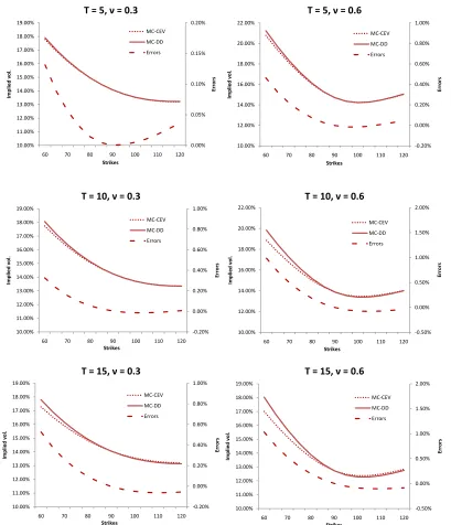
We have systematically investigated the mapping under different regimes and scenarios when strikes are not far from at the money. In the results presented here, the parameters are taken to be consistent with our later numerical study and representative enough so that similar results are expected to hold for all cases.
0.00%
Figure 2.1: Effects of maturity T and Volvol ν on the mapping when the ATM are matched. Parameters: β = 0.5, ρ=−0.2, σ0 = 130%, F0 = 90. MC-CEV: CEV-SABR MC solution, MC-DD:
-0.50%
Figure 2.2: Effect of very long maturityT on the mapping when the ATM are matched. Parameters:
β = 0.5, ρ=−0.2, σ0= 130%, F0= 90.
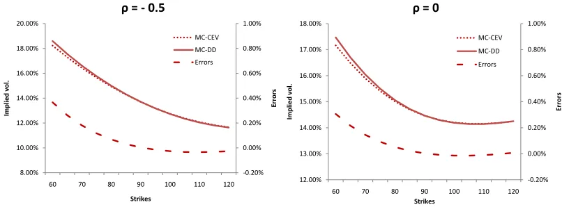
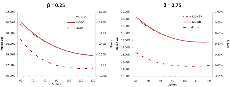
We mentioned that both ρ and β affect the skew. In figure 2.3, it is seen that the correlation parameterρ does not really affect the mapping and the error curves look almost identical. On the other hand,β as illustrated in figure 2.4 has a stronger influence and the mapping tends to be less accurate for smaller β. This makes sense since perfect mapping is obtained as β approaches one. For low value of β, the displaced diffusion coefficient θ is large enabling more probability mass to be assigned to negative values ofFT while the absorbing barrier of the CEV structure also plays a more significant role.
-0.20% 0.00% 0.20% 0.40% 0.60% 0.80% 1.00%
10.00% 12.00% 14.00% 16.00% 18.00% 20.00% 22.00%
60 70 80 90 100 110 120
Er
ro
rs
Im
p
lied
vol
.
Strikes
β = 0.25
MC-CEV
MC-DD Errors
-0.20% 0.00% 0.20% 0.40% 0.60% 0.80% 1.00%
10.00% 11.00% 12.00% 13.00% 14.00% 15.00% 16.00% 17.00% 18.00% 19.00%
60 70 80 90 100 110 120
Er
ro
rs
Im
p
lied
v
o
l.
Strikes
β = 0.75
MC-CEV MC-DD
Errors
Figure 2.4: Effect of β on the mapping when the ATM are matched. Parameters: ρ =−0.2, T = 10, ν = 0.3, F0 = 90, σ0 is chosen for each case so that the ATM are comparable.
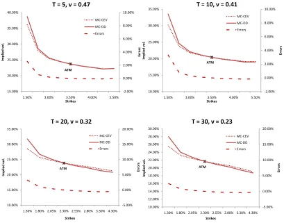
2.1.2 Implied volatilities in the wings
We have further investigated the behaviour in the wings. In the results presented here, the pa-rameters are taken to represent typical market swaption smiles of different maturities (figure 2.5). We chose to work with swaption data as strikes being far from at the money is observed more often in the interest rate market. While high strikes are not really a problem, the gap between two models gets bigger as the strike gets lower. When the strike is sufficiently low (ATM - 200 bp), the error can approach 3 to 4% which is quite significant in practice. For increasing maturity (20 and 30 years), the mapping completely breaks down for “ATM - 200 bp” strike even with very low ν. This fact was addressed in Svoboda-Greenwood (2009) in detail. The author argues that even in the deterministic volatility setting, the mapping may work well given the assumption that forward interest rates are “not too low” and their percentage volatilities are “reasonable”. When such assumption fails, a greater portion of the probability density function is likely to fall in the negative rates region for the DD process while a large part of the distribution is absorbed at zero for the CEV process over intermediate maturities. These effects become more pronounced for longer maturity. We report these results for the data used in figure 2.5 in table 2.1. For the 20 year maturity case, it is seen that around a quarter of the mass is given to the absorbing barrier and a fifth to the negative rates region. Therefore, the mapping can no longer be justified. We want to stress that this is not really a problem as both models are not good enough in practice here.
ATM
1.50% 3.00% 3.50% 4.00% 5.50%
Er
1.50% 3.00% 3.50% 4.00% 5.50%
Er
1.30% 1.80% 2.05% 2.30% 2.55% 2.80% 3.30% 4.30%
Strikes
1.30% 1.80% 2.05% 2.30% 2.55% 2.80% 3.30% 4.30%
Strikes
CEV-SABR 5.18 % 9.77% 25.85% 30.15% DD-SABR 4.03 % 7.67% 19.47% 22.60%
Table 2.1: Probability mass assigned to the absorbing barrier (CEV-SABR) and the negative rates region (DD-SABR) for the four cases considered in figure 2.5 (computed by direct Monte Carlo simulation).
3
A probabilistic approximation
3.1 Approximating the terminal distribution
By the fundamental pricing formula and tower property, today’s numeraire-rebased price of a Vanilla call option struck at some strike K is given by
C0(K, F0) = E(FT −K)+
= EE{(FT −K)+|σT}
. (3.1.1)
double integral. Recall that σT has a known Log-Normal distribution as the SDE it solves has an explicit solution. To keep the notation simple and transparent, we introduce the process s that represents the level of assets and function g(.) to transform it back to the underlying process F, i.e. Ft=g(st). As the first stepping stone, we will write down the exact solutions in distribution to the SDE for our reference models (see Appendix A for details).
• Normal SABR:
• Log-Normal SABR:
sT , lnF0+
0 σt2dt is the realized variance andGis a standard Normal random variable indepen-dent of σT and VT. We aim to approximate the conditional distribution of sT|σT by replacing it with some suitable random variable with the same conditional mean and variance. In each case, the realized variance VT plays a central role in our calculation and analysis so we will treat its moments separately in the following proposition.
Proposition 1 Assume that the dynamics of the volatility is governed by a Log-Normal process with Volvol ν > 0, i.e. dσt = νσtdZt where Z is a Brownian motion. The first two conditional
moments of the realized variance VT have the following analytical expressions:
E(VT|σT) =
where φ(.) and Φ(.) are the Normal density and cumulative distribution functions respectively.
3.2 Normal approximation
We first consider the Normal distribution for the approximation ofsT|σT as it appears to be very tractable and efficient to use in practice. Another motivation for choosing the Normal distribu-tion comes from an earlier numerical investigadistribu-tion in Mitra (2010). In this work, the condidistribu-tional distribution of sT|σT was seen to be quite close to Normal through examination of the Q-Q plots (see section 3.3 for further discussion). In order to implement this approximation, we first need to calculate the exact conditional mean and variance ofsT
µ(σT) = E(sT|σT),
η2(σT) = Var(sT|σT),
and then replace the conditional distribution of sT|σT by a Normal random variable with mean
µ(σT) and varianceη2(σT). One will then be able to calculate the call option prices by (3.1.1) and obtain the implied volatilities. The analytical formulae for µ(σT) and η2(σT) are quoted in the following proposition.
Proposition 2 : The conditional mean and variance of sT for the reference models are given by
the following closed-form expressions:
• Normal SABR:
µ(σT) = F0+
• Log-Normal SABR and DD-SABR:
µ(ˆσT) = ln(F0+θ) +
3.2.1 Implementation: advantages and disadvantages
We apply the formulae derived in the last section to the direct calculations of Vanilla call option prices for all strikes. Since there is a one to one correspondence between the volatility process σ
and its driving Brownian motion Z (through the SDE ofσ)
ZT =
ln(σT/σ0) +12ν2T
ν ,
ZT ∼ N(0, T),
we can also express the conditional mean and variance in terms of ZT. Consequently, the inner conditional expectation in (3.1.1) has the equivalent expressionE(FT −K)+|ZT
and (3.1.1) now reads
C0(K, F0) =
Z ∞
−∞E
[(g(sT)−K)+|ZT =x]fZT(x)dx,
where g(.) is the appropriate transformation for the chosen β and fZT(x) = e
−x2
2T/ √
2πT is the probability density function of ZT. After some direct calculations we obtain:
1. Normal SABR:
C0(K, F0) =
Z ∞
−∞
" p
η2(x)φ K−µ(x)
p
η2(x)
!
+ (µ(x)−K) 1−Φ Kp−µ(x)
η2(x)
!!#
e−x
2 2T √
2πTdx.
(3.2.3) 2. Log-Normal SABR:
C0(K, F0) =
Z ∞
−∞
"
eµ(x)+η2(2x)Φ µ(x) +η
2(x)−lnK
p
η2(x)
!
−KΦ µ(px)−lnK
η2(x)
!#
e−x
2 2T √
2πTdx.
(3.2.4)
Remark 1 : For the DD-SABR model, we have exactly the same formula as (3.2.4)withK replaced by K+θ.
Both (3.2.3) and (3.2.4) are simple one-dimensional integrals and can therefore be evaluated easily by some efficient numerical routine. We want to emphasize this point because we think it is crucial. Although the Normal approximation, as we shall see later, does not appear to be the best choice theoretically, it is the only one that could compete with other asymptotic approximations in terms of computational time and this is an important consideration for any practical model. Consequently, one should always look at the regimes when it works well and not so well. Despite its convenience and simple form, the Normal approximation admits a potential numerical problem as described in the following remark.
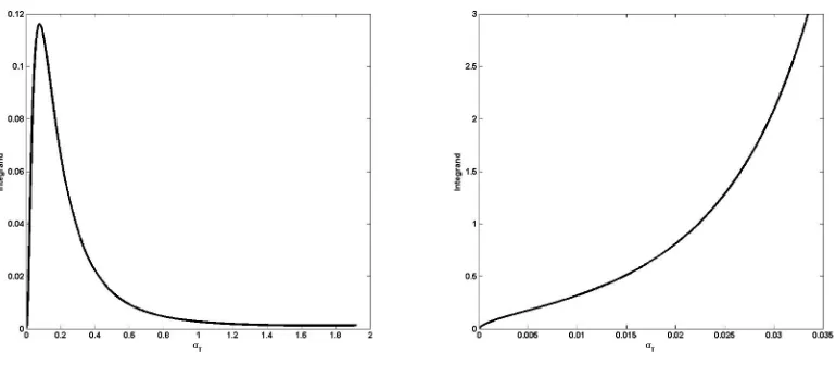
Remark 2 : For both the Log-Normal SABR and DD-SABR models, E(VT2|σT) and henceη2(σT)
become very large when ν2T is large can be observed from equation (3.1.6). For certain parameter choices, the growth rate of E[(g(sT)−K)+|ZT =x] in equation (3.2.4) is not balanced by the rate
Figure 3.1: The integrand of (3.2.4) as a function of σT. Left plot: β = 1, ρ=−0.5, F0= 90, K =
90, T = 10, ν = 0.3, σ0 = 15%, right plot: β = 1, ρ=−0.5, F0 = 90, K = 90, T = 15, ν = 0.6, σ0 =
15%.
As a result, prices can not be calculated correctly when the numerical convergence fails. In principle, one can do the following
C0(K, F0) =
Z ∞
−∞E
[(g(sT)−K)+|ZT =x]
e−x
2 2T √
2πTdx
≈
Z z
z
E[(g(sT)−K)+|ZT =x]
e−x
2 2T √
2πTdx,
where z and z are the appropriate lower and upper limits for the numerical integration. For some regimes of large ν2T, z cannot be chosen to give the numerical convergence. In practice, one can truncate the integral at a much lowerz to avoid this issue as the volatility process is unlikely to hit a very high level at maturity. If the truncated value is too low, the density function will have to be re-normalized, that is
C0(K, F0) =
Z z
z
E[(g(sT)−K)+|ZT =x] ˜fZT(x)dx,
˜
fZT(x) =
e−x
2 2T
Rz z e
−u2 2T du
.
3.2.2 A comparison with other approximations
Authors Normal SABR Log-Normal SABR CEV-SABR DD-SABR Hagan et al. (2002) tested tested tested not tested Obloj (2008) tested tested tested not available Paulot (2009) not tested not tested tested not available Johnson et al. (2009) not available tested not tested not available Wu (2010) tested tested tested not available Larsson (2010) tested tested not available tested
Table 3.1: Check list of the most current approximations for the SABR model.
The SABR formula in Hagan et al. (2002) is the original and, perhaps, the most popular amongst the listed works in this table owing to its algebraic closed-form expression. Henceforth, we take the SABR formula as the benchmark approximation for our comparison. In the SABR formula, the Black implied volatility σB(K, S0) for a Vanilla call (or put) option written on the
forward priceS struck at some strikeK has the following form
σB(K, F0) =
The ATM Black implied volatility reduces to
σB(F0, F0) =σ0F0β−1
We borrow the same technique † to derive an equivalent Black implied volatility formula for the DD-SABR model (see Appendix D)
σB(K, F0) = ˆσ0
where
andx(z) has the same form as (3.2.6). For the special case of the ATM option, the formula reduces to
For the rest of the paper, we will refer to (3.2.8) and (3.2.9) as the DD-SABR formula. One can immediately recognize a lot of similarities between this formula and the SABR formula given strikes near the money and short maturity. A systematic comparison of the Normal approximation with the SABR and DD-SABR formulae will be addressed in section 4. Meanwhile, we summarize the results of other established approximations in conjunction with the SABR formula and emphasize the Normal approximation’s superiority.
Most of the approximations listed in table 3.1 fail or lose their precision whenT >10 years even with low ν, e.g. both Wu (2010) and Larsson (2010) focus on maturity less than 5 years or Paulot (2009) completely breaks down for ν2T >1.6. The reason is that most of the techniques (singular perturbation or heat kernel expansion) are based on the assumption of small total volatility ν2T‡
to allow for accurate asymptotic expansions up to the second order. As discussed in section 3.2.1, the total volatilityν2T also affects the Normal approximation to some extent. An intuitive reason for this adverse effect is that a larger value of ν2T will push the true conditional distribution of sT|σT further away from Normal. However, in the results presented in section 4, the Normal approximation is shown to perform quite well for the Normal SABR model up to 30 years maturity or very large ν2T ≈ 10.8. For the other sub-models, it works well up to 15 years maturity or
ν2T ≈1.8. A further advantage of the Normal approximation over the current approaches is that
it always yields a proper density function for the underlying while the other techniques sometimes result in negative density at the low strike region for long maturity, e.g. the SABR formula. This issue is addressed in Obloj (2008) and Johnson et al. (2009) but the problem still remains.
3.3 Normal Inverse Gaussian approximation
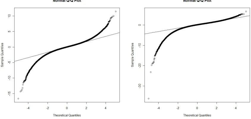
As hinted previously, the true conditional distribution of sT|σT can be far from Normal for some parameter sets. We track down this flaw by looking at the Q-Q plots of the standardized conditional
‡
sample ofsT|σT against the standard Normal distribution. In figure 3.2, the results show that even when the Normal approximation works, the true conditional distribution displays much heavier tails than the Normal distribution. We even observe more left skewness asσT gets bigger.
Figure 3.2: Normal Q-Q plots: standardized conditional samples of sT|σT against the standard Normal distribution. Common parameters: β = 1, ρ = −0.5, F0 = 90, σ0 = 5%. left plot: T =
15, ν = 0.3, σT = 5%, right plot: T = 15, ν = 0.3, σT = 50%.
The breakdown of the Normal approximation for certain parameter choices leads us to a further investigation of a more flexible distribution which can capture the skewness and heavy tails. We propose the Normal Inverse Gaussian (NIG) distribution for such purpose. NIG is quite popular in finance, especially in the financial econometrics literature, for instance Barndorff-Nielsen (1997).
Under the NIG approximation, we assume
sT|σT ∼ N IG( ˆα,β,ˆ µ,ˆ δˆ),
where the parameters are to be chosen. The NIG density function is defined as follows:
fN IG(s; ˆα,β,ˆ µ,ˆ δˆ) = ˆ
α
ˆ
δ exp(ˆδ
q ˆ
α2−βˆ2−βˆµˆ)
K1
ˆ
αδˆq1 + (s−ˆµˆ δ )
2
q
1 + (s−ˆµˆ δ )
2
exp( ˆβs), (3.3.1)
where s ∈ R and each parameter has a specific role: ˆα > 0 determines the tail heaviness of the distribution, ˆδ > 0 is the scale parameter, ˆµ∈ R is the location parameter, and |βˆ|<αˆ controls the asymmetry of the distribution. The functionK1(.) is the modified Bessel function of the third
3.3.1 Matching Parameters
We now describe an efficient way to match the NIG parameters. We use the fact that a NIG random variableX can be expressed as the Normal variance-mean mixture form:
X= ˆµ+ ˆβY +
√
Y G, (3.3.2)
where the mixing random variableY follows an Inverse Gaussian (IG) distribution (see Barndorff-Nielsen (1997)) andGis a standard Normal random variable that is independent of Y. If
Y ∼ IG(ˆδ,
q ˆ
α2−βˆ2),
E(Y) =
ˆ
δ
q ˆ
α2−βˆ2
,
Var(Y) = δˆ q
ˆ
α2−βˆ2
3,
then
X∼ N IG( ˆα,β,ˆ µ,ˆ ˆδ).
Therefore, matching the mean and variance of the mixing random variable is adequate to capture those of the corresponding NIG random variable. It is clear from (3.1.2) and (3.1.4) that conditioned on σT,sT will have a similar form as (3.3.2). We will now express the NIG parameters in terms of
σT.
• For β = 0: the mixing random variable is (1−ρ2)VT|σT. We first match the location and asymmetry parameters
ˆ
µ(σT) = F0+
ρ
ν(σT −σ0),
ˆ
β(σT) = 0.
• For 0< β≤1: the mixing random variable is (1−ρ2)β2F02β−2VT|σT. Similarly, we have that ˆ
µ(σT) = ln(F0+θ) +
ρ νβF
β−1
0 (σT −σ0),
ˆ
β(σT) = − 1 2(1−ρ2).
It now remains to derive ˆδ(σT) and ˆα(σT) by matching the conditional mean and variance of the mixing random variable, i.e.
• Forβ = 0
ˆ
δ(σT) q
ˆ
α2(σ
T)−βˆ2(σT)
= (1−ρ2)E(VT|σT),
ˆ
δ(σT) q
ˆ
α2(σ
T)−βˆ2(σT)
3 = (1−ρ
2)2Var(V
• For 0< β≤1
ˆ
δ(σT) q
ˆ
α2(σ
T)−βˆ2(σT)
= (1−ρ2)β2F02β−2E(VT|σT),
ˆ
δ(σT) q
ˆ
α2(σ
T)−βˆ2(σT)
3 = (1−ρ
2)2β4F4β−4
0 Var(VT|σT).
As there are only two unknowns, solving the above simultaneous equations is a straightforward task.
3.3.2 Implementation: two-dimensional integration
Unlike the Normal approximation, we have to perform a two-dimensional integration in order to compute the Vanilla call prices using the NIG approximation. Note that as the NIG parameters can be expressed in terms ofZT, we have that
C0(K, F0) =
Z ∞
−∞
Z ∞
−∞
(g(s)−K)+fN IG(s; ˆα(x),βˆ(x),µˆ(x),δˆ(x))ds
e−x
2 2T √
2πTdx
= Z ∞
−∞
Z ∞
g−1(K)
(g(s)−K)fN IG(s; ˆα(x),βˆ(x),µˆ(x),δˆ(x))ds
e−x
2 2T √
2πTdx, (3.3.3)
where g(.) (specified in (3.1.2), (3.1.3) and (3.1.4)) is the appropriate transformation and g−1(.) denotes its inverse. Although the above double integral could be a bottleneck in computation and numerically more expensive than the Normal approximation, the implementation scheme is actually quite straightforward. We apply the Simpson’s rule, which is found sufficient to give the numerical convergence, to evaluate both the inner and outer integrals. When numerically integrating the outer integral, the upper limitz (discussed in the implementation for the Normal approximation) can be taken to be quite comfortably large and we do not have the same problem as the Normal approximation. This is because the growth rate of the inner integral is much slower than the rate of decay offZT(·). Consequently, their product always tends to zero in the tails of distribution of
ZT. The lower limit z, on the other hand, has to be chosen with more care. For short maturity, if too low a value of z is taken, the NIG parameters can be undefined. This is not really a problem as very small probability mass is assigned to those small values. However, for longer maturity z
has to be sufficiently small to preserve the probability mass.
Efficiency: One can improve the efficiency of the NIG implementation by the following scheme. Recall that the inner integral of (3.3.3) has the following form
I(x, K) = Z ∞
g−1(K)
(g(s)−K)fN IG(s; ˆα(x),βˆ(x),µˆ(x),δˆ(x))ds
where fN IG is given by (3.3.1). For ease of exposition, we write fN IG(s; ˆα,β,ˆ µ,ˆ ˆδ) instead of
fN IG(s; ˆα(x),βˆ(x),µˆ(x),δˆ(x)) but implicitly mean the dependence of the NIG parameters on x. By change of variable, we set
y:= ˆαδˆ
s 1 +
s−µˆ ˆ
δ
2
Hence
It can be easily checked thatH(.) is a smooth function inyfor each fixed set of the NIG parameters and strike K. Therefore, one can approximateH(.) by a piecewise polynomial of the form
H(y, K) =
the NIG approximation as follows
• For a grid ofx values, store the coefficients{an(x), bn(x)}mn=0.
1(y)dycan be evaluated by polynomial interpolation between the grid values
li−1 andli.
4
Numerical study
In this section, we investigate the quality of the approximations developed in this paper. It is known that both the Normal and Log-Normal SABR models can be implemented quite well with the SABR formula so we will compare the Normal and NIG approximations with this formula. Similarly for the DD-SABR model, we will test them against the DD-SABR formula.
We take the Monte Carlo solutions (denoted MC for both the Normal and Log-Normal SABR models, and MC-DD for the DD-SABR model) of the SDEs as a natural benchmark to compare all the approximations against. In our numerical study, the initial volatility σ0 is first chosen to
represent the level of the true ATM implied volatility (≈σ0F0β−1). We force all the ATM implied
volatilities produced by the approximations to be the same as the Monte Carlo ATM by adjusting
σ0 and compare errors along the wings as practitioners do in practice.
4.1 Normal SABR
We consider the typical parameter values: β = 0, ρ=−0.1, F0 = 90, σ0 = 9 for varying maturities
T. Since the Normal and NIG approximations work very well for the Normal SABR model, as we shall see in the coming plots, we present our results for the large Volvol cases only and better results are expected to hold for typical market volatility regimes.
-2.00%
Figure 4.1: Effects of maturity within a high Volvol regime on the Normal and NIG approximations. Other parameters: β= 0, ρ=−0.1, F0 = 90, ν = 0.6, σ0 = 9. The dashed curve of the same colour
Strike
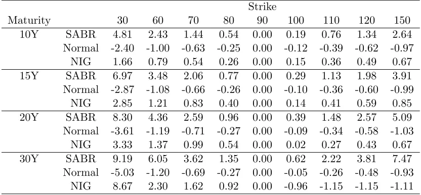
Maturity 30 60 70 80 90 100 110 120 150
10Y SABR 4.81 2.43 1.44 0.54 0.00 0.19 0.76 1.34 2.64 Normal -2.40 -1.00 -0.63 -0.25 0.00 -0.12 -0.39 -0.62 -0.97
NIG 1.66 0.79 0.54 0.26 0.00 0.15 0.36 0.49 0.67 15Y SABR 6.97 3.48 2.06 0.77 0.00 0.29 1.13 1.98 3.91 Normal -2.87 -1.08 -0.66 -0.26 0.00 -0.10 -0.36 -0.60 -0.99
NIG 2.85 1.21 0.83 0.40 0.00 0.14 0.41 0.59 0.85 20Y SABR 8.30 4.36 2.59 0.96 0.00 0.39 1.48 2.57 5.09 Normal -3.61 -1.19 -0.71 -0.27 0.00 -0.09 -0.34 -0.58 -1.03
NIG 3.33 1.37 0.99 0.54 0.00 0.02 0.27 0.43 0.67 30Y SABR 9.19 6.05 3.62 1.35 0.00 0.62 2.22 3.81 7.47 Normal -5.03 -1.20 -0.69 -0.27 0.00 -0.05 -0.26 -0.48 -0.93
NIG 8.67 2.30 1.62 0.92 0.00 -0.96 -1.15 -1.15 -1.11
Table 4.1: Fitting errors, in percentages, against strike and maturity for β = 0, ν = 0.6, ρ =
−0.1, F0 = 90, σ0 = 9 (approximation implied volatility minus MC volatilities).
Comments on the accuracy of approximations: for β= 0,
• The SABR formula starts losing precision for T ≥ 10 years while the Normal and NIG approximations still perform quite well and remain relatively close up to 30 years maturity. All the approximations perform worse on the left wing of the implied volatility curves but the errors are still acceptably small for the Normal and NIG approximations (table 4.1). The errors only become substantial when we consider 30 years maturity and low strike (30). Note that in this case, ν = 0.6 represents a highly stress market condition forT = 10,15,20 and 30 years.
• The Normal approximation does not display enough curvature while the SABR formula shows the opposite. The plots show that it is always a lot closer to the MC solution than the SABR formula on both wings. Furthermore, the errors of the Normal approximation are recorded to be very stable across maturities.
• Similar to the Normal approximation, the NIG approximation works well up to very long maturity even within a high volatility regime, i.e. very highν2T ≈10. As maturity increases from 20 years to 30 years, the implied volatility curve produced by the NIG approximation becomes progressively steeper. It is observed in this case that the Normal approximation is a better choice than the NIG approximation.
4.2 Log-Normal SABR and DD-SABR
Since the Log-Normal SABR and DD-SABR models yield a lot of similarities in structure, we present their numerical results together and single out the volatility regimes when each individual approximation performs well. We consider the typical parameter values:
• β = 0.5, F0= 90, ρ=−0.2, σ0= 130%.
Figure 4.2 displays the moderate maturity cases where the Normal approximation still performs quite well.
Figure 4.2: Effects of moderate maturity within a low Volvol regime on the Normal and NIG approxmations. Common parameters: ν = 0.3, F0 = 90, top: β = 1, σ0 = 15%, ρ=−0.5, bottom
β = 0.5, σ0 = 130%, ρ = −0.2. The dashed curve of the same colour indicates the errors of the
corresponding approximation.
2.00%
Figure 4.3: Effects of very long maturity within a low Volvol regime on the NIG approximation. Common parameters: ν = 0.3, F0 = 90, top: β = 1, σ0 = 15%, ρ = −0.5, bottom: β = 0.5, σ0 =
-2.00% 0.00% 2.00% 4.00% 6.00% 8.00% 10.00%
5.00% 10.00% 15.00% 20.00% 25.00% 30.00%
60 70 80 90 100 110 120
Er
ro
rs
Im
p
lie
d
v
o
l.
Strikes
T = 15,
= 0.6
DD-SABR
MC-DD
NIG
Figure 4.4: Effect of high ν2T (stress volatility regime) on the NIG approximation. Parameters:
β = 0.5, ν = 0.6, S0 = 90, σ0 = 130%, ρ=−0.2. The dashed curve of the same colour indicates the
errors of the corresponding approximation.
Comments on the accuracy of approximations: for 0< β≤1
• Asβ varies from 1 to 0, the Normal and NIG approximations perform better.
• The SABR formula starts breaking down when T ≥ 10 years or ν2T ≥ 0.9 as the left and right wings of implied volatility curves are not in line with the MC solutions. On the contrary, the Normal approximation maintains similar shape and therefore fits the MC curves much better than the SABR formula for these cases. It works well up to 15 years and only breaks down for very long maturity or ν2T >1.8.
• The NIG approximation seems to work well up to ν2T ≈ 3.6 and 5.4 for β = 1 and 0.5 respectively with the error plots having the lowest magnitude compared with the others. These upper bounds forν2T are obtained from the following case analysis:
– Low Volvol (ν ≈ 0.3): the NIG approximation performs well up to 30 years maturity for β = 0.5 and slightly away from the MC solution for β = 1. Note that in this case,
ν ≈0.3 is the typical market volatility regime forT ≥20 years.
– High Volvol (ν ≈ 0.6): it starts breaking down when T > 15 years for β = 0.5 and
T > 10 years for β = 1. The plots show that the errors are reasonably small with slightly wrong curvature. In this case,ν ≈0.6 represents the stress volatility regime for moderate maturity.
exact (MC-DD) results for the cases considered in section 2.1.2. It is seen from this table that the mass given by the NIG approximation and the MC-DD solution are very close while that given by the Normal approximation is a bit higher. This supports our findings in this section that the NIG approximation is closer in distribution to the MC-DD solution than the Normal approximation.
T 5 Y 10 Y 20 Y 30 Y
MC-DD 4.03 % 7.67% 19.47% 22.60% Normal 4.37% 8.22% 22.06% 24.91% NIG 4.29% 7.49% 18.36% 21.73%
Table 4.2: Probability mass assigned to the negative rates region for the four cases considered in figure 2.5.
5
Conclusions
Using an entirely probabilistic framework, we have derived a new approximation for the terminal distribution of the underlying asset. In our method, the main objective is to model the asset’s distribution at the maturity date rather than the implied volatilities themselves. This is necessary if we want to extend the approximation to the pricing of more exotic derivatives. The results show that simple approximations which allow for ease of computation are rich enough to capture the model’s terminal distribution. The benchmark models we considered in this paper are the SABR model and the DD-SABR model. In section 2, we find that the CEV-SABR and the DD-SABR model with chosen matching parameters produce very similar implied volatility curves provided that maturity is not too long. Although they are not as close for other cases, we still can work with both models to achieve similar objectives.
References
Barndorff-Nielsen, O. E. (1997). Normal Inverse Gaussian Distributions and Stochastic Volatility Modelling. Scandinavian Journal of Statistics,24(1), 1-13.
Berestycki, H., Busca, J., & Florent, I. (2004). Computing the implied volatility in stochastic volatility models. Comm. Pure Appl. Math.,57(10), 1352-1373.
Black, F., & Scholes, M. (1973). The pricing of options and corporate liabilities.Journal of Political Economy,81(3), 637-659.
Cox, J. C. (1996). The constant elasticity of variance option pricing model. Journal of Portfolio Management,23, 15-17.
Hagan, P., Kumar, D., Lesniewski, A., & Woodward, D. (2002). Managing smile risk. Wilmott Magazine,1(8), 84-108.
Hagan, P., Lesniewski, A., & Woodward, D. (2005). Probability distribu-tion in the SABR model of stochastic volatility. Preprint.. (Available at http://lesniewski.us/papers/working/ProbDistrForSABR.pdf)
Henry-Labordere, P. (2005). A general asymptotic implied volatility for stochastic volatility models.
SSRN eLibrary.. (Available at http://papers.ssrn.com/sol3/papers.cfm?abstractid= 698601) Johnson, S., & Nonas, B. (2009). Arbitrage-free construction of the swaption cube.
http://ssrn.com/abstract=1330869.
Joshi, M., & Rebonato, R. (2003). A displaced diffusion stochastic volatility LIBOR market model: motivation, definition and implementation. Quantitative Finance,3(6), 458-469.
Karatzas, I., & Shreve, S. (1991). Brownian motion and stochastic calculus, 2nd edition. Springer-Verlag, Berlin, Heidelberg and New York.
Larsson, K. (2010). Dynamic Extensions and Probabilistic Expansions of the SABR model.
http://ssrn.com/paper=1536471.
Marris, D. (1999). Financial option pricing and skewed volatility. Unpublished master’s thesis, University of Cambridge.
Mitra, S. (2010). A One Factor Approximation for the SABR model. Unpublished master’s thesis, Warwick Business School, University of Warwick.
Obloj, J. (2008). Fine-tune your smile: Correction to hagan et al. Wilmott Magazine,35, 102-104. Paulot, L. (2009). Asymptotic Implied Volatility at the Second Order with Application to the SABR
model. http://ssrn.com/abstract=1413649.
Piterbarg, V. (2005). Stochastic volatility model with time-dependent skew. Applied Mathematical Finance,12:2, 147-185.
Rebonato, R. (2002). Modern pricing of interest-rate derivatives. Princeton University Press. Rubinstein, M. (1983). Displaced diffusion option pricing. Journal of Finance,38(1), 213-217. Schroder, M. (1989). Computing the constant elasticity of variance option pricing formula. Journal
of Finance,44(1), 211-219.
Svoboda-Greenwood, S. (2009). Displaced diffusion as an approximation of the constant elasticity of variance. Applied Mathematical Finance,16(3), 269-286.
A
Distribution of
F
Tunder the Log-Normal SABR model
The SDE of the Log-Normal SABR model is
dFt = σtFtdWt,
dσT = νσtdZt,
dWt = ρdZt+ p
1−ρ2dWˆt,
whereZ and ˆW are independent Brownian motions. By Itˆo’s lemma, we have that
lnFT = lnF0+ By considering the conditional moment generating function (m.g.f) ofMT, we have that
E eaMTFT
by using the tower and “taking out what is known” properties. Hence
lnFT ,lnF0+
The same steps follow in both the Normal SABR and DD-SABR models to obtain (3.1.2) and (3.1.4) respectively.
B
Proof of Proposition 1: conditional moments of the realized
variance
V
TTo calculateE(VT |σT) andE(VT2 |σT) we use the concept of a Brownian Bridge. By Itˆo’s lemma, we have that:
ZT =
ln(σT/σ0) +12ν2T
Hence, ifσT is known, the value of the end point ZT is immediate.
Conditional on ZT, we have a Brownian bridge whose values at time zero and T are known. Define
whereBtis a standard one-dimensional Brownian motion thenZt|ZT is a Brownian bridge from 0 toZT on [0, T] (Karatzas & Shreve (1991)). It then follows from equation (B.0.3) that
Zt|σT =Zt|ZT ∼ N
and it has the following covariance function for 0≤t, s≤T
Cov(Zt, Zs|σT) =t∧s−
ts
T. (B.0.5)
B.1 First conditional moment of VT
The conditional expectation of the realized variance can now be written in the following form:
E(VT |σT) = E
where Φ is the cumulative normal distribution function. Plugging back (B.0.2) to (B.1.1), we obtain
E(VT |σT) =
B.2 Second conditional moment of VT
We now evaluate the second conditional moment of the realized variance.
By completing the square and change of variableu= 2ν√(t+s)
in the inner integral of (B.2.1), we have that
E(VT2 |σT) = 2σ04exp
Putting all the pieces together we obtain
C
Proof of proposition 2: conditional mean and variance of
s
TWe prove the Log-Normal SABR case only as similar calculations apply to other models. The
conditional meanof sT is
µ(σT) = E(sT|σT) The conditional varianceofsT:
η2(σT) = Var(sT|σT) Similarly, the covariance term in (C.0.6) can be expressed as
Cov(VT, V
and the last term in (C.0.6) is
again using the tower property and noting thatE(G2) = 1. Hence
η2(σT) = 1 4E(V
2
T|σT)− 1
4[E(VT|σT)]
2
+ (1−ρ2)E(VT|σT). (C.0.7)
Given the formulae from the previous appendix, the results follow immediately.
D
DD-SABR equivalent Black implied volatility
In this appendix, we derive an equivalent Black implied volatility formula for the DD-SABR model using the techniques developed in Hagan et al. (2002) but with a few modifications from later literature, e.g. Hagan et al. (2005), Obloj (2008). We start with a more general form of the SABR model:
dFt = σˆtC(Ft)dWt,
dσˆt = νσˆtdZt,
dZtdWt = ρdt,
where the function C(u) is is assumed to be positive, smooth and integrable around 0: Z x
0
du
C(u) <∞, x >0.
Equation (B.65) in appendix B of Hagan et al. (2002) yields the equivalent Black implied volatility for the above model:
σB(K, F0) =
ˆ
σ0lnF0/K
RF0
K du C(u)
z x(z)
× (D.0.8)
( 1 +
"
2γ2−γ12+F12
av
24 σˆ
2
0C2(Fav) +
1
4ρνˆσ0γ1C(Fav) +
2−3ρ2
24 ν
2
#
T+. . .
)
.
Here
Fav = p
F0K, (D.0.9)
γ1 =
C0(Fav)
C(Fav)
, (D.0.10)
γ2 =
C00(Fav)
C(Fav) , (D.0.11)
and
z = ν
ˆ
σ0
F0−K
C(Fav),
x(z) = ln ( p
1−2ρz+z2+z−ρ
1−ρ
)
,
criticisms of this function z, e.g. Obloj (2008). We use a more general form of z as proposed in Hagan et al. (2005).
z= ν
Note that for this choice of z, implied volatilities obtained by this approximation coincide with Berestycki et al. (2004) and Obloj (2008) for the CEV-SABR model. We now turn our attention to the DD-SABR model as introduced in the main paper. The model is the special case:
C(Ft) = Ft+θ,
Making this substitution in (D.0.10), (D.0.11) and (D.0.12) we obtain:
γ1 =
Substituting further in (D.0.8), we get:
σB(K, F0) =
We can simplify this formula by expanding§ (F0+θ)−(K+θ) =
Hence, the implied volatility formula now reads
σB(K, F0) = ˆσ0
For the special case of ATM options, we first take the limit
lim K→F0
lnF0/K
ln(F0+θ)/(K+θ)
= F0+θ
F0
, (D.0.13)
and hence the formula reduces to
σB(F0, F0) = σˆ0
F0+θ
F0
1 +
2θ/F0+θ2/F02
24 σˆ
2
0 +
1
4ρνσˆ0+
2−3ρ2
24 ν
2
T +. . .
= σ0F0β−1
1 +
21−ββ +(1−ββ2)2
24 σ
2
0β2F
2β−2
0 +
1
4ρνσ0βF β−1
0 +
2−3ρ2
24 ν
2
T+. . .
= σ0F0β−1
1 +
1−β2
24 σ
2
0F
2β−2
0 +
1
4ρνσ0βF β−1
0 +
2−3ρ2
24 ν
2
T+. . .