Wave Diffraction Problem from a Semi-Infinite Truncated Cone
with the Closed End
Dozyslav B. Kuryliak1, *, Kazuya Kobayashi2, and Zinoviy T. Nazarchuk1
Abstract—The electromagnetic wave diffraction from the modified cone formed by a circular truncated cone whose aperture is closed by a spherical cap is considered. The problem is reduced to the solution of the mixed boundary value problem for the Helmholtz equation. The axially symmetric version of the problem, where the cone is excited by a radial electric dipole (E-polarization wave diffraction problem), is analyzed. A new approach to the solution is proposed. The solution includes the application of the Kontorovich-Lebedev integral transformation, the nonstandard procedure for derivation of the Wiener-Hopf equation and its reduction to the set of linear algebraic equations of the second kind. Their solution ensures the fulfillment of all the necessary conditions including the edge condition. The approximate equation for the sharp truncated cone terminated by the spherical cap is analyzed. The low frequency approximation as well as the transition to the plane which incorporates the hemispheric cavity is analysed. The numerical calculation results are presented.
1. INTRODUCTION
We consider the scattering of electromagnetic waves from a closed truncated cone. The cone consists of the semi-infinite cone with a cut vertex and an open end which is closed by the spherical cap; the spherical radius and the angle of this cap are equal to the spherical radius and to the angle of the conical hole respectively. The conical scatterer created by this way possesses the sharp rectangular circular edge; the edge is formed by the orthogonal coordinate surfaces in the spherical coordinate system. This is a canonical problem of the wave diffraction theory. The rigorous solution of this problem has broad applications depending on the geometrical parameters; the modeling of the reflector and horn antennas as well as of the semi-spherical cavities at the plane surface for modeling of the cavity type defects are also included. Nevertheless, the existing literature focuses mainly on the wave diffraction from the closed finite cone; it is a cone open end which is closed by the spherical cap. The mode matching technique is mainly used for the analysis of this problem [1–3]. It is well known that the singularity of field components at the edge for such structure behaves like ρ−1/3 as ρ → 0, where ρ is the distance to the edge in the local coordinates. This determines the asymptotic behaviour of the magnitudes for expansion modes as xn =O(n−2/3) ifn→ ∞. This feature, as a rule is not taken into account in well the known mode matching technique. For the potential theory the finite closed cone was analysed by the Wiener-Hopf technique in [4]. The one-sided or two-sided closed structures in the rectangular and cylindrical coordinates like the cavities or rods are studied rigorously using the Wiener-Hopf technique in the Fourier transform domain [5–10]. The application of this powerful tool for the solution of the mentioned problems in the rectangular and cylindrical coordinates is not standard because of the existence of the boundary condition at the lateral plane surfaces. In this paper
Received 10 October 2018, Accepted 25 November 2018, Scheduled 6 December 2018
* Corresponding author: Dozyslav B. Kuryliak ([email protected]).
1 Department of Physical Bases of Materials Diagnostics, Karpenko Physico-Mechanical Institute of NAS of Ukraine, 5 Naukova Str.,
we develop the Wiener-Hopf technique for the rigorous solution of the wave diffraction problem for a closed truncated cone. This is a new canonical problem, which is much more complicated due to the involvement of the Kontorovich-Lebedev (K-L) integral transformation. For the potential theory semi-infinite truncated hollow cone was analysed by the Wiener-Hopf technique and the Mellin integral transform in [11]. The Wiener-Hopf technique and the K-L integral transform were earlier applied to the solution of the wave diffraction problems for finite and semi-infinite truncated hollow cones [12–15]. A particular case to these problems namely the wave diffraction from the disc was analysed by this method in [16]. In [17] the K-L integral transform for the finite interval [18] and the Wiener-Hopf technique were applied to the analysis of the scattering characteristics of the finite cone in spherical perfectly conducting resonator. The analytical regularization technique for the solution of the different kinds of the wave diffraction problems was considered for hollow conical scatterers excited by the electromagnetic and acoustic waves in [14, 19–24]. Earlier in [25] we analysed the wave diffraction by the openended conical cavity formed by the truncated cone with the internal spherical diaphragm. This structure excited axially-symmetrically by the radial electric dipole and the resonance scattering of the different kinds of the open sphere-conical resonators were studied. The analytical regularization technique was applied to obtain the solution. The technique applied earlier does not allow for the rigorous analysis of the clear closed truncated cone. Here this problem is solved rigorously by the Wiener-Hopf technique.
2. FORMULATION OF THE PROBLEM
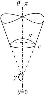
In spherical coordinates (r, θ, ϕ) let us consider an axially symmetric electromagnetic wave diffraction by the perfectly conducting semi infinite truncated cone closed by the spherical cap as
Q={c < r <∞ forθ=γ and r=c forγ < θ≤π} (1) (see Fig. 1). The coordinate ϕ∈ [0,2π) is omitted in this notation. The cone in Eq. (1) is excited by the radial electric dipole that is located at the conical axis. The time factor is assumed to bee−iωt and is suppressed throughout this paper.
Figure 1. Geometry of the problem.
Let us formulate our problem in terms of the scalar Debye potential and express the nonzero field components outside ofQ in the form
Er =−(r sinθ)−1∂θ(sinθ∂θU), Eθ =r−1∂rθ(rU),
Hϕ =ikZ−1 ∂θU,
(2)
Next, we reduce the wave diffraction problem to the solution of the boundary value problem for
the Helmholtz equation as
∇2+k2U = 0, (3)
which is valid outside the closed truncated cone; its solution satisfies the boundary conditions
(r sinθ)−1∂θ
sinθ ∂θU(t)
= 0, ifθ=γ, c < r <∞, (4a)
r−1∂rθ
r U(t)
= 0, ifγ < θ≤π, r=c, (4b)
as well as the radiation condition in the Sommerfeld form and the condition at the rectangular circular edge [5, 6, 10] in form Eθ, Er(r,γ) ∼ |β1(θ−γ) +β2(c−r)|−1/3, if r → c, θ → γ, where β1, β2 are
constants to be determined by the strength of the source; the obtained solution must be regular at r= 0.
Here the symbol∇2 denotes the Laplace operator in spherical coordinates for the axial symmetric case
∇2 =
r−2∂rr2∂r+ (r2sinθ)−1∂θ(sinθ ∂θ),
U(t) =U(t)(r,θ) is the total field. We suppose that the cone in Eq. (1) is excited by the radial electric dipole that is located at the conical axisθ= 0. Taking this into account, let us determine the total field as
U(t)=
U(i)+U, if 0≤θ < γ,
U, if γ < θ≤π, (5)
whereU(i)=U(i)(r, θ) is the incident field excited in the semi-infinite perfectly conducting circular cone due to the radial electric dipole with coordinater =l >0 at the conical axis, which is taken in the form
U(i)= A
(e) 0
πi√sr
Γ∗
ν[Pν−1/2(cosγ)Pν−1/2(−cosθ)−Pν−1/2(−cosγ)Pν−1/2(cosθ)]
cos(πν)Pν−1/2(cosγ)
Kν(sl)Iν(sr)dν, (6)
if 0≤θ < γand U(i)≡0 whenγ < θ≤π. Here Γ∗∈Π is a vertical straight line in the regularity strip
Π ={ν :|Reν|<1/2};s=−ik;Pν−1/2(·) is the Legendre function of the first kind;Iν(·),Kν(·) are the
modified Bessel and Macdonald functions respectively; A(0e)=A0/(l
√
sl), where [A(0e)] =V,A0 =πp0Z
is the known value, and p0 is the dipole moment. Integral (6) is absolutely convergent for θ <2γ. If
ν ∈ Π, the arguments of the modified Bessel and Macdonald functionssr and sl can be also swapped without the changing of this integral.
3. FIELD REPRESENTATION IN THE TRANSFORM DOMAIN
Let us introduce the Kontorovich-Lebedev (K-L) integral transform as
F(ν) = K{φ (r);ν}=
∞
0
φ(r)Kν(sr)√drr, (7a)
φ(r) = K−
1
{F(ν); r}= 1 π i√r
Γ∗ν F
(ν)Iν(sr)dν, (7b)
where Re(s) ≥ 0 and φ(r) = O(rq1) with q1 > −1/2, if r → 0 and φ(r) = O(rq2) with q2 ≤ −1, if r→ ∞, Γ∗ ∈Π. Hence F(ν) is the regular function in the strip Π. For the further analysis we assume that Re(s) >0 and Im(s) = 0 to ensure the convergence of the K-L integral transforms. The solution for real k(s=−ik) will be obtained at the end of the analysis.
Let us define the K- L transform of the scattered fieldU(r,θ), if 0≤θ < γas follows
Φ(ν,θ) =
∞
0
Applying the K-L transform to Eq. (3), we find that the function in Eq. (8) satisfies the ordinary differential equation
1 sinθ
d
dθ sinθ d
d θ Φ(ν,θ)
+ (ν2−1/4)Φ(ν,θ) = 0, (9)
the general solution of which bounded at θ= 0 is
Φ(ν,θ) =A(ν)Pν−1/2(cosθ), if 0≤θ < γ. (10)
HereA(ν) is an arbitrary function to be determined from the boundary conditions. For our convenience, let us rewrite Eq. (10) as
Φ(ν,θ) =E(ν, γ − 0) Pν−1/2(cosθ) (ν2−1/4)P
ν−1/2(cosγ),
(11)
whereE(ν,γ−0) is the K-L transform of the electric fieldEr(r,γ−0) which is defined as
E(ν,γ−0) = c
0
rEr(r,γ−0)Kν(sr)√dr
r. (12)
This follows from the boundary condition in Eq. (4a) and the definition of the incident field in Eq. (6). Due to the separation of variables U(t)(r, θ) = U1(t)(r)U
(t)
2 (θ), the total field representation of Eq. (5)
and the assumption that∂θU2(t)(θ)= 0, ifγ < θ≤π, we get the following correlation from the boundary
condition in Eq. (4b)
∂cU(c, θ) =−c−1U(c, θ), ifγ < θ≤π. (13) Applying the K-L transformation to Eq. (3), ifγ < θ≤π we arrive at the equation
1 sinθ
d
dθ sinθ d
d θΦ1(ν,θ)
+ (ν2−1/4)Φ1(ν,θ) =c∂c √
cKν(sc)U(c,θ), (14)
wherec∂c[√cKν(sc)]U(c,θ) is the unknown inhomogeneous term;
Φ1(ν,θ) =
c
0
U(r,θ)Kν(sr)√dr
r. (15)
Let us introduce the K-L integral in the form
Φ2(ν,θ) =
c
0
U(r,θ)Iν(sr)√dr
r. (16)
The function in Eq. (16) satisfies the differential Eq. (14) with the unknown inhomogeneous term as c ∂c[√cIν(sc)]U(c,θ). Then, the function
F(ν,θ) = Φ1(ν,θ)∂c √
c Iν(sc)−Φ2(ν,θ)∂c √
c Kν(sc) (17)
that is formed by using the correlations in Eqs. (15), and Eq. (16) satisfies the homogeneous differential Eq. (9), the solution of which bounded forγ < θ≤π looks as follows
F(ν, θ) =B(ν)Pν−1/2(−cosθ). (18)
Here B(ν) is an arbitrary function to be determined from the boundary conditions.
Taking into account the representation in Eq. (18), let us rewrite Eq. (17) in the form
F(ν, θ) =E1(ν,γ+ 0)∂c √
cIν(sc)−E2(ν,γ+ 0)∂c √
cKν(sc) Pν−1/2(−cosθ) (ν2−1/4)P
ν−1/2(−cosγ).
HereE1(2)(ν,θ) =−(sinθ)−1∂θ[sinθ ∂θΦ1(2)(θ)] or, as follows from the definitions in Eqs. (15), (16) and
first correlation in Eq. (2),
E1(ν,γ+ 0) =
c
0
rEr(r,γ+ 0)Kν(sr)√dr
r, (20a)
E2(ν,γ+ 0) =
c
0
rEr(r,γ+ 0)Iν(sr)√drr. (20b)
Then, we use the boundary condition in Eq. (4a) as well as the condition of the continuity for tangential electric fields atθ=γ and deriveEr(r,γ−0) =Er(r,γ+ 0) =Er(r,γ) for 0< r < c and
E(ν,γ−0) =E1(ν,γ+ 0) =E1(ν,γ), (21)
where
E1(ν,γ) =
c
0
rEr(r,γ)Kν(sr)√dr
r. (22)
Equations (11), (19) are the desired field representation in the K-L transform domain that are regular in the strip Π.
4. WIENER-HOPF EQUATION
For the tangential magnetic fields it follows from the boundary condition that
Hϕ(t)(r, γ+ 0) − Hϕ(t)(r, γ−0) =
0, if 0< r < c, j1(r), if c < r <∞.
(23)
Applying the K-L transform to Eq. (23) we receive
J1(ν, γ) =H(ν, γ+ 0)−H(ν, γ−0) =− ∞
c
Hϕ(t)(r, γ−0)Kν(sr)√dr
r, (24)
where
J1(ν, γ) = ∞
c
j1(r, γ)Kν(sr)√dr
r (25)
is the even entire function and
H(ν,γ−0) =
∞
0
Hϕ(t)(r,γ−0)Kν(sr)√dr
r, H(ν,γ+ 0) = c
0
Hϕ(t)(r,γ+ 0)Kν(sr)√dr
r. (26)
Taking into account Eqs. (11) and (15), we represent Eq. (24) as
(iωε)−1J1(ν,γ) = Φ1(ν,γ+ 0)−Φ(ν,γ−0)−Φ(i)(ν,γ). (27)
Here
Φ(ν, γ−0) = lim
θ→γ−0∂θΦ(ν, θ), Φ
1(2)(ν, γ+ 0) = limθ→γ+0∂θΦ1(2)(ν, θ), (28)
and
Φ(i)(ν,γ) = A
(e) 0
√ s
Pν−1/2(cosγ)∂γPν−1/2(−cosγ)−Pν−1/2(−cosγ)∂γPν−1/2(cosγ)
cos(πν)Pν−1/2(cosγ)
Kν(sl) (29)
Differentiating correlations in Eqs. (11), (19) with respect to θ and setting θ =γ ±0, we obtain from the expressions (21), (17) that
Φ(ν, γ−0) = E1(ν, γ)
∂γPν−1/2(cosγ)
(ν2−1/4)P
ν−1/2(cosγ),
(30a)
Φ1(ν,γ+ 0) = Φ2(ν,γ+ 0){ √
scKν(sc)} {√scIν(sc)}
+
E1(ν,γ)−E2(ν,γ+ 0){
√
scKν(sc)} {√scIν(sc)}
×
× ∂γPν−1/2(−cosγ)
(ν2−1/4)P
ν−1/2(−cosγ)
. (30b)
Considering the definition in Eq. (5) and the representation in Eq. (16) let us introduce the new notation as
Φ2(ν,γ+ 0) = 1
iωεH2(ν,γ), (31)
where
H2(ν, γ) =
c
0
Hϕ(t)(r, γ+ 0)Iν(sr)√drr =iωε ∂γ c
0
U(r, γ+ 0)Iν(sr)√drr. (32)
Taking into account the known relationship [26]
Pν−1/2(−cosγ)∂γPν−1/2(cosγ)−Pν−1/2(cosγ)∂γPν−1/2(−cosγ) =
2 cos(πν) πsinγ , we rewrite Eq. (29) as
Φ(i)(ν, γ) =− 2 πsinγ
A(0e)Kν(sl)
√
sPν−1/2(cosγ).
(33)
Then, substituting correlations in Eqs. (30), (31), and (33) into Eq. (27) and taking into account the equality in Eq. (32), we arrive at
E1(ν, γ)M(ν, γ) +E2(ν, γ+ 0)
πsinγ ∂γPν−1/2(−cosγ)
2(ν2−1/4)P
ν−1/2(−cosγ)
{√scKν(sc)} {√scIν(sc)} −
− A
(e) 0 Kν(sl)
√
sPν−1/2(cosγ)
=−πsinγ 2iωε
J1(ν, γ)−H2(ν, γ){
√
scKν(sc)} {√scIν(sc)}
, (34)
where
M(ν, γ) = cos(πν)
(ν2−1/4)P
ν−1/2(cosγ)Pν−1/2(−cosγ)
. (35)
Here M(ν, γ) is the even meromorphic function without zeros in the strip of regularity Π; if |ν| → ∞, M(ν, γ) tends to zero in Π as ν−1. Out of Π the function M(ν, γ) possesses the real simple zeros at ν =±zn(≡n+ 1/2) and poles at ν = ±νn and ν =±μn (n = 1,2, 3, . . .) that are determined from the solution of the transcendental equations
Pνn−1/2(cosγ) = 0, (36a)
Pμn−1/2(cosγ) = 0. (36b)
The asymptotic behaviour of the roots of these equations, ifn→ ∞ is as follows [26]:
νn=π(n−1/4)/γ+O(1/n), μn=π(n−1/4)/(π−γ) +O(1/n). (37) Equation (34) is the desirable form of the representation of the Wiener-Hopf equation of the problem; E1(ν, γ),E2(ν, γ+0) andJ1(ν, γ),H2(ν, γ) are the unknown functions that are regular at least forν∈Π.
5. SOLUTION OF THE WIENER-HOPF EQUATION
Using the known relation between the modified Bessel functions of the first and the second kind we represent the unknown function in Eq. (21) as follows [16]
E1(ν, γ) =
1 2E
+ 1(ν, γ)
sc
2
ν
Γ(−ν) +1 2E
− 1 (ν, γ)
sc
2
−ν
Γ(ν), (38)
where Γ(·) is the Gamma function,
E1±(ν, γ) = Γ(1±ν) sc
2
∓νc
0
rEr(r, γ)I±ν(sr)√dr
r. (39)
Since the asymptotic representation of the modified Bessel function looks as I±ν(sr) ∼ (sr/2)±ν/Γ(1±ν), if |ν/sr| >> 1 and taking into account the function Er(r, γ) = O(1) if r → 0, we obtain that
E1±(ν, γ)≤C1 1
0
x1/2±νdx= C1 3/2±ν,
where x=r/c <1 and C1 = const. From this it follows that the functions E1±(ν, γ) are regular in the
complex overlapping half-planes Re(ν)><−3/32/2 respectively.
Taking into account thatEr(r,γ)∼(c−r)−1/3 along the conical rim (r→c−0, θ=γ), we find as
E1±(ν, γ)≤C2 1
0
x1/2±ν(1−x)−1/3dx=C2B(±ν+3/2,2/3) =O(ν−2/3), Re(ν)>− 3/2
<3/2 and |ν| → ∞,
whereC2 = const,B(z,y) is the beta-function [27].
The kernel function M(ν, γ) is factorized as
M(ν, γ) =M+(ν, γ)M−(ν, γ), (40)
where M±(ν, γ) are split functions regular and nonzero in Re(ν)<>1−/12/2, M+(ν, γ) = M−(−ν, γ) and
M±(ν, γ) =O(ν−1/2) as |ν| → ∞with Re(ν)><1−/12/2;
M−(ν, γ) =B0
(1/2−ν)Γ(1/2−ν)e−ν χ
∞
n=1
(1−ν/ξn)eν/ξn
−1
,
with {ξn}∞n=1 ={νp}∞p=1∪ {μk}∞k=1 is the growing sequence; νn and μn for n= 1,2,3, . . . denotes the positive roots of the transcendental Eqs. (36a) and (36b),
B0 = i
√
π{P−1/2(cosγ)P−1/2(−cosγ)}−1/2,
χ = γ πln
γ π +
π −γ
π ln
π −γ
π −ψ(3/4)−S(γ)−S(π −γ),
S(γ) =
∞
n=1
γ
π(n−1/4) − 1 νn
, S(π−γ) =
∞
n=1
π−γ π(n−1/4) −
1 μn
and ψ(·) is the logarithmic derivation of the Gamma function [27]. Using the correlations in Eqs. (20b), (21), and (39) we derive
E2(ν, γ+ 0) = E + 1 (ν, γ)
Γ(1 +ν)
sc
2
ν
Let us substitute the equality in Eq. (38) into Eq. (34) and multiply both sides of the obtained equation by 2(sc/2)νM+−1(ν, γ)Γ−1(ν). Then using Eq. (41) we arrive at
E1−(ν, γ)M−(ν, γ) +E +
1 (ν, γ)M−(ν, γ)
Γ(−ν) Γ(ν) (sc/2)
2ν+
+E1+(ν, γ)
Υ1(ν, γ)(sc/2)2ν
M+(ν, γ)Pν−1/2(−cosγ)
{√scKν(sc)} {√scIν(sc)} −
A√(0e)
s Λ(ν, sl, sc, γ) =
=−πsinγ iωε
J1(ν, γ)(sc/2)ν
M+(ν, γ)Γ(ν)
+ Ω
+
1 (ν, γ, sc)(sc/2)2ν
M+(ν, γ)
{√scKν(sc)} {√scIν(sc)} .
(42)
Here ν∈Π1;
Υ1(ν, γ) =
πsinγ ∂γPν−1/2(−cosγ)
(ν2−1/4)Γ(ν)Γ(1 +ν) , (43a)
Λ(ν, sl, sc, γ) = Kν(sl) (sc/2) ν
M+(ν, γ)Pν−1/2(cosγ)Γ(ν),
(43b)
Ω+1(ν, γ, sc) = πsinγ iωε
H2+(ν, γ)
Γ(ν)Γ(1 +ν), (43c)
where
H2+(ν, γ) = Γ(1 +ν)(sc/2)−νH2(ν, γ). (43d)
Let us consider the function as
h+(ν, γ) = J1(ν,γ) M+(ν,γ)Γ(ν)
(sc/2)ν. (44)
Here J1(ν,γ) is determined in Eq. (24) and is the entire function in the complex plane ν.
Taking into account the asymptotics of the Macdonald’s function Kν(sr) ∼ Γ(±ν)(sr/2)∓ν/2, if Re(ν) → ±∞ and by using the Stirling’s formula for the Gamma function as well as the edge condition for Hϕ(t)(r, γ + 0), j1(r) ∼ (c − r)2/3, if r → c, we find from Eqs. (25), (26) that
H2+(ν, γ), h+(ν, γ) are regular functions in the half-plane Re(ν) ≥ 0. These functions tend to zero,
if |ν| → ∞, in all the regularity region; for Re(ν) > 1 H2+(ν, γ) ∼ B(ν + 1 1 2,1
2
3) = O(ν−
5/3) and
h+(ν, γ)∼ν1/2B(ν−1, 123) =O(ν−7/6). Then we find that all terms in the right-hand part of Eq. (42) are regular functions at least in Re(ν)≥0 and tend to zero, if|ν| → ∞, in the regularity region. The first term in the left-hand part of Eq. (42) is a regular function in the complex half-plane Re(ν)<1/2. All three rest terms in this part of Eq. (42) are regular in the strip Π1 and tend to zero, if |ν| → ∞ in
this strip. In order to arrange Eq. (42) into the Wiener-Hopf form, it is necessary to decompose each of these three terms into the sum of two functions regular in the left-hand and the right-hand half-planes overlapping on strip Π1 due to the relation
[· · ·]∓=± 1 2π i
i∞+iε1
−i∞+iε1
[· · ·] dν
ν−α, (45)
where 0< ε1<1/2; Re(α)< ε1 and Re(α)> ε1 for upper and lower signs respectively. In Eq. (42), we
split the terms that are regular in the overlapping half-planes and place them on the opposite sides of the equality symbol. Thus, we form the entire function which, according to the Liouville’s theorem, is identical to zero. Then, we arrive at
E−1(α, γ)M+(α,γ) +
1 2πi
i∞+ε1
−i∞+ε1
E+1(ν, γ)M−(ν,γ)
Γ(−ν) Γ(ν) (sc/2)
2ν dν
ν−α+
+πsinγ 2πi
i∞+ε1
−i∞+ε1
E+1(ν,γ)∂γPν−1/2(−cosγ) (sc/2)2ν{
√
scKν(sc)} (ν2−1/4)M
+(ν,γ)Pν−1/2(−cosγ)Γ(ν)Γ(1+ν){
√
scIν(sc)} dν ν−α =A
(e) 0 f(α).
For convenience we introduced the notationE±1(α, γ) =
√
sE1±(α, γ); Re(α)< ε1;
f(α) = 1 2πi
i∞+ε1
−i∞+ε1
Λ(ν, sl, sc, γ) dν
ν−α. (47)
It is seen that the singularities associated with the first and second integrands in Eq. (46) for Re(ν)> ε1 are simple poles, ifν =n,ξn, andν =μnrespectively withn= 1,2,3, . . .. The singularities
of the integrand Eq. (47) for Re(ν)> ε1 are the simple poles at ν =νn. Then, evaluating the integral
by enclosing the contour into the right half-plane after some manipulations we derive
E−1(α, γ)M−(α, γ) + ∞
n=1
(−1)nE+1(n, γ)M−(n, γ)(sc/2)2n
Γ(n)Γ(n+ 1)(n−α) +
+
∞
n=1
πE+1(ξn, γ)(sc/2)2ξn
Γ(ξn)Γ(ξn+ 1) sin(πξn)[M−−1(ξn, γ)](ξn−α) +
+2πsinγ
∞
n=1
E+1(μn, γ)Pμ1n−1/2(−cosγ){
√
scKμn(sc)}/{
√
scIμn(sc)}(sc/2)2μn
(μ2
n−1/4)Γ(μn)Γ(μn+ 1)M+(μn, γ)(μn−α)∂μPμn−1/2(−cosγ)
=f(α)A(0e),
(48)
where
f(α) =−
∞
n=1
Kνn(sl) (sc/2)νn
Γ(νn)M+(νn,γ)(νn−α)∂νPν−1/2(cosγ)|ν=νn
. (49)
The series in the left-hand side of Eq.(48) is absolutely convergent for any parameters of the cone and the series in Eq. (49) is absolutely convergent, if l > c. In order to derive the second kind linear algebraic system, we set α=−p,α=−νp,α=−μp in Eq. (48),p= 1,2,3, . . .. This procedure leads to the three sets of linear algebraic equations as follows
x(1)p +
∞
n=1
b(11)pn x(1)n +
∞
n=1
b(12)pn x(2)n +
∞
n=1
b(13)pn x(3)n =fp(1), ..
.
x(2)p +
∞
n=1
b(21)pn x(1)n +
∞
n=1
b(22)pn x(2)n +
∞
n=1
b(23)pn x(3)n =fp(2), ..
.
x(3)p +
∞
n=1
b(13)pn x(1)n +
∞
n=1
b(23)pn x(2)n +
∞
n=1
b(33)pn x(3)n =fp(3).
.. .
(50)
Here x(pq) = E
+ 1(η
(q)
p ), x(pq) = O(p−2/3), if p → ∞; ηp(1) = p, η(2)p = νp, ηp(3) = μp, p = 1,2,3, . . .; fp(q)=f
−η(q)
p
A(0e)/M+
ηp(q), γ
,q = 1,2,3;
b(pnq1) = (−1) nM
−(n, γ) (sc/2)2n
Γ(n)Γ(n+ 1)M+
η(pq), γ n+ηp(q)
,
b(pnq2) = π(sc/2)
2νn
Γ(νn)Γ(νn+ 1) sin (πνn)M+(η(pq), γ)
M−−1(νn,γ)
νn+ηp(q)
,
b(pnq3) = π(sc/2)
2μn
Γ(μn)Γ(μn+ 1)M+(ηp(q), γ)(μn+η(pq))
1
+ 2sinγP
1
μn−1/2(−cosγ){
√
scKμn(sc)}
(μ2
n−1/4)M+(μn,γ)∂μPμn−1/2(−cosγ){
√
scIμn(sc)}
.
Let us consider the version l < c. In this case, let us represent expression (47) as
f(α) = 1 2πi
2
p=1
i∞+ε1
−i∞+ε1
Λp(ν, sl, sc, γ) dν
ν−α, (51)
where
Λ1(ν, sl, sc, γ) =
Γ(1−ν)I−ν(sl) 2M+(ν,γ)Pν−1/2(cosγ)
sc
2
ν
, (52a)
Λ2(ν, sl, sc, γ) = − πIν
(sl)
2 sin(πν)Γ(ν)M+(ν,γ)Pν−1/2(cosγ) sc
2
ν
. (52b)
We evaluate the integrals in Eq. (51) by enclosing their contours into the left half-plane for the first integral; the singularities associated with the first integrand for Re (ν) < ε1 are simple poles at
ν =α and ν = −zn with n= 1,2,3, . . .. In the second integral Eq. (51) we evaluate enclosing the contour into the right-half plane; the singularities associated with the second integrand for Re(ν)> ε1
are simple poles at ν =n and ν = νn with n = 1,2,3, . . .. Taking these into account and using the residue theorem we arrive at
f(α) = Γ(1−α)I−α(sl) (sc/2) α
2M+(α, γ)Pα−1/2(cosγ)
+
∞
n=1
Γ(1 +zn)Izn(sl) (sc/2)−zn
2{M−(zn, γ)}Pzn−1/2(cosγ)(zn+α)
+
+
∞
n=1
(−1)nIn(sl) (sc/2)n
2Γ(n)M+(n, γ)Pn−1/2(cosγ)(n−α)
+
+
∞
n=1
πIνn(sl) (sc/2)νn
2 sin(πνn)Γ(νn)M+(νn, γ)∂νPνn−1/2(cosγ)(νn−α)
.
(53)
Here f(α) is a regular function in the left complex half-plane (Re(α)<0); the series included into this function are absolutely convergent, ifl/c <1. In order to derive the second kind linear algebraic system from Eq. (48) we need to determine the function in Eq. (53) at α=−p(−νp,−μp) forp= 1,2,3, . . .. It is necessary to note that the first term in the right-hand side of the equality in Eq. (53) is limited at α = −νp because lim
α→ −νpM+(α,γ)Pα−1/2(cosγ) = ∂αPνp−1/2(cosγ)/
M−−1(νp,γ) = 0 and the singularity of this term atα=−znis suppressed by the singularity of the n-th term of the first series in Eq. (53). Ifα=−μp, the first term in the equality of Eq. (53) equals zero because lim
α→−μpM+(α, γ)→ ∞.
6. TRANSITION TO THE HEMISPHERIC CAVITY WITH A FLANGE (γ =π/2)
For this particular case the wave diffraction problem is reduced to the key relations in Eq. (48) with the kernel function in Eq. (35) as
M(ν, π/2) =M+(ν, π/2)M−(ν, π/2) =
Γ2(ν/2 + 3/4)Γ2(−ν/2 + 3/4) (ν2−1/4)Γ(ν+ 1/2)Γ(−ν+ 1/2).
Here
M±(ν, π/2) =i 2
±νΓ2(±ν/2 + 3/4)
(±ν+ 1/2)Γ(±ν+ 1/2),
where M−(ν, π/2), M+(ν, π/2) are split functions regular in the overlapping semi-planes Re(ν)<1/2,
Re(ν) > −1/2; their simple zeros and poles are located in the supplemental half planes at zn = ±(2n+ 1/2), ξp = ±(2p−1/2) respectively, p, n = 1,∞; M−(ν, π/2) = M+(−ν, π/2) = O(ν−1/2), if
7. TRANSITION TO THE SHARP TRUNCATED CONE
The obtained set of linear algebraic equations gives the exact solution to the Wiener-Hopf Eq. (34). The three first terms in the left-hand side of Eq. (48) describe the wave diffraction from the aperture of the semi-infinite truncated cone and the forth term identifies the wave diffraction from the spherical cap termination. It is easy to see that for the thin conical wire (γ →π) the last term in the left-hand side of this equation decreases and can be omitted; in these cases we neglect the effects of wave interaction with the spherical cap and arrive at
E−1(α, γ)M−(α, γ) + ∞
n=1
(−1)nE
+
1(n, γ)M−(n, γ)(sc/2)2n
Γ(n)Γ(n+ 1)(n−α) +
+
∞
n=1
πE+1(ξn, γ)(sc/2)2ξn
Γ(ξn)Γ(ξn+ 1) sin(πξn)M−−1(ξn, γ)(ξn−α)
=A(0e)f(α). (54)
This equation coincides with the early obtained equation for the solution of the wave diffraction problem by the hollow truncated cone with any opening angle [14, 15].
8. LOW-FREQUENCY APPROXIMATION
For this purpose let us consider the solution of our problem for static limit (|s| → 0). To find this solution, we introduce the new unknown functions
X±(ν, γ) = lim s→0
E±1(ν,γ)= 0.
Using the asymptotic behaviour of the modified Bessel functions and their derivatives for the small argument, we arrive at
{√scKμn(sc)}
{√scIμn(sc)}
∼ −(2μn−1)Γ(μn)Γ(μn+ 1) 2(2μn+ 1)
sc
2
−2μn
. (55)
Let us substitute Eq. (55) into Eq. (48). Then, taking into account Eqs. (49), (53) and neglecting the terms with (sc/2)2ηn, ηn =n, (νn, μn) we arrive at the linear algebraic system, which keeps only the unknowns X+(μp,γ), where p= 1,2,3, . . .. as
X+(μp,γ)−sinγ
∞
n=1
bpnX+(μn,γ) =dp, (56)
where
bpn = π(2μn−1)P
1
μn−1/2(−cosγ)
(μ2
n−1/4)(2μn+ 1)(μn+μp)M+(μp,γ)M+(μn,γ)∂μPμn−1/2(−cosγ),
(57a)
dp = A
(e) 0
2M+(μp,γ) ⎧ ⎪ ⎪ ⎪ ⎪ ⎨ ⎪ ⎪ ⎪ ⎪ ⎩
−∞ n=1
(c/l)νn
Γ2(νn)M
+(νn,γ)(νn+μp)∂ν Pν−1/2(cosγ)ν=νn
, if l > c,
∞
n=1
(l/c)zn
{M−(zn,γ)}Pzn−1/2(cosγ)(zn−μp)
, if l < c.
(57b)
The unknownsX+(p,γ),X+(ν
9. FIELD REPRESENTATION
Let us turn to determination of the wave fieldU(r, θ) for 0≤θ≤γ, 0< r <∞. Applying the inverse K-L transform to Eq. (8) and taking into account Eqs. (11), (21) and (38), we derive that
U(r, θ) =U1(r, θ) +U2(r, θ). (58)
Here
U1(r,θ) =
1 2πi√sr
Γ∗
E+1(ν,γ)
νPν−1/2(cosθ)Γ(−ν)
(ν2−1/4)P
ν−1/2(cosγ) sc
2
ν
Iν(sr)dν, (59a)
U2(r,θ) =
1 2πi√sr
Γ∗
E−1(ν,γ)
νPν−1/2(cosθ)Γ(ν)
(ν2−1/4)P
ν−1/2(cosγ) sc
2
−ν
Iν(sr)dν, (59b)
where Γ∗⊂Π.
It is seen that the singularities associated with the integrands Eqs. (59a) and (59b) for Re(ν)><Γ∗ are the simple poles at ν =±1/2,ν =±n,ν=±νn with n= 1,2,3, . . ., respectively. Then, evaluating the integral Eqs. (59a) and (59b) by enclosing the contour into the right and left half-planes respectively and applying the residue theorem we arrive at the representation of the field potential in Eq. (58) in form as
U(r,θ) =−√2 sr
∞
n=1
E+1(νn,γ) (sc/2)νnPνn−1/2(cosθ)
(ν2
n−1/4)Γ(νn)∂ν Pν−1/2(cosγ)ν=νn
Kνn(sr). (60)
Here r > c and the terms associated with the poles at ν = ±1/2 are omitted because they are independent of coordinate θ and do not contribute to the field components representation. To obtain this formula the terms associated with the residues of the integrands in Eqs. (59a) and (59b) atν =n and ν = −n respectively were canceled, and the terms associated with the residues at ν = νn and ν =−νn were used for the formation of the Macdonald’s functionKνn.
The correlation in Eq. (60) allows for obtaining the field components anywhere forr > cin the form of absolutely convergent series using the relations in Eq. (2). Taking this into account and applying the estimation of the solutions of Eq. (50), we find that the singularity of the normal to the conical edge field components is
lim
r→c+0, θ=γ|Er|,|Eθ| ≤C ∞
n=1
E+1(νn, γ)
e−nπγ |ln(c/r)|∼ |ln(c/r)|−1/3, (61)
whereC is the known constant. Then, the expression for far-field patterns looks as follows
Hϕ =Z−1Eθ =D(θ)eikr/r for r→ ∞. (62)
Here D(θ) = D1(θ) +
D2(θ), where
D1(θ) and
D2(θ) are Hϕ far field distribution for diffracted and
incidence fields respectively,
D1(θ) =
√ 2πZ−1
∞
n=1
E+1(νn,γ) (sc/2)νnPν1n−1/2(cosθ)
(ν2
n−1/4)Γ(νn)∂ν Pν−1/2(cosγ)ν=νn
, (63a)
D2(θ) = −
√
2πZ−1A(0e) ∞
n=1
νnPνn−1/2(−cosγ)Iνn(sl)Pν1n−1/2(cosθ)
cos(πνn)∂ν Pν−1/2(cosγ)ν=νn
. (63b)
For the next numerical analysis we suppose that the cone would be placed in the hypothetical environment with the unit dielectric and magnetic parameters excited by the dipole field in Eq. (6) withp0k= 1/(4π) [A].
(b) (a)
(d) (c)
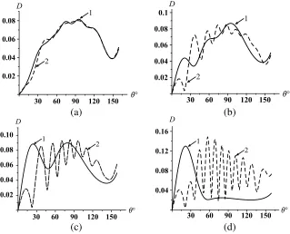
Figure 2. Far-field pattern of the closed truncated cone with kc = 18, γ = 160◦; (a) kl = 0.5; (b)kl= 9.0; (c) kl= 12.0; (d) kl= 17.0; dipole location: (1)r=l,θ= 180◦, (2) r=l,θ= 0◦.
which is placed at the axis of the symmetry of the cone. The shadow region of this reflector is limited by the conical surface; the cone forms the barrier for wave penetration into the region γ < θ ≤π. In Figs. 2(a)–(d) the numerical examples of the total far field D=|D(θ)| with 0≤θ≤γ are shown. For the convenience of this study, we represent the features of the far field formation by the two curves in each of the Figs. 2(a)–(d) with the same parameter kl; curves 1 and 2 show the total far fields, if the dipole is located at the axis θ = π and θ = 0 or, in other words, if the dipole is located closer to or further from the reflector. From these figures we observe how the changes of the dipole location at these axes influence|D(θ)|. Thus, the behaviour of the curves in these figures for the narrow flange spherical reflector (γ = 160◦) weakly influences the dipole far field distribution in the semi-infinite conical region, if its location is not far from center of the scatter (r = 0) for both semi-axes θ = π and θ = 0 (see Fig. 2(a)).
Let us shift the dipole at the axis θ=π closer to the reflector. This leads to weak oscillations of the far field (see curves 1, Figs. 2(b), (c), (d)), the effective radiation into the narrow sector of angles spanning the axis θ = 0◦, and to the formation wide angle area, where the field practically does not penetrate (see curve 1, Fig. 2(d)). This effect could be explained by the focusing properties of the concave spherical mirror. Let us put the dipole at the axisθ= 0 and move it further from the reflector. In this case, we observe sharp oscillations of the far field for all the observation angles (see curves 2 in Figs. 2(c), (d)). This shows the intensive interference of the waves scattered from different elements of our structure, such as the circular edge, conical and concave spherical surfaces.
In order to confirm our conclusions we analyse the wider reflector with the opening angleγ= 130◦ and the same radius kc= 18. We find the similar scattering properties (see Figs. 3(a)–(d)). Note that curves 1 in Figs. 3(c), (d) show the far-field patterns of the dipole which is encompassed by the spherical mirror because kccos(π−γ)< kl.
Similar to the characteristics in Fig. 2(d), we find the effective radiation near the axis θ = 0 and the formation of the wide angle area, into which the field practically does not penetrate (see curves 1, Figs. 3(c), (d)). We also observe the sharp oscillations of the far field, if the dipole is located at the axisθ= 0 and moves further from the aperture (see curves 2, Figs. 3(c), (d)).
(b) (a)
(d) (c)
Figure 3. Far-field pattern of the closed truncated cone with kc = 18, γ = 130◦; (a) kl = 0.5; (b)kl= 6.0; (c) kl= 12.0; (d) kl= 17.0; dipole location: (1)r=l,θ= 180◦, (2) r=l,θ= 0◦.
(b) (a)
(d) (c)
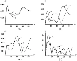
Figure 4. Far-field pattern of the closed truncated cone with kc = 18, γ = 89◦; (a) kl = 0.1; (b)kl= 3.0; (c) kl= 6.0; (d) kl= 12.0; dipole location: (1) r=l,θ= 180◦, (2)r =l,θ= 0◦.
Let us consider the scatter Q withγ < π/2 which is the model for the analysis of wave radiation from the spherical resonator into the semi-infinite conical horn; it is important to maximize the radiated power into the horn. For this purpose we analyse the radiation of the resonance modes that can be excited in the closed spherical resonator through the circular hole in the conical horn. Radiations trough the circular hole in the spherical resonator in continuum were analysed early in [28]. In Figs. 5(a), (b) the radiation of the T M10n resonance mode into the conical horns with the different opening angles is
shown. Here the indexes n= 1,2,3,4 determine the number of the corresponding spherical resonance radiuses for the closed spherical resonator; all these resonance modes are similarly dependent on the polar angle θ as P11(cosθ) = −sinθ [27]. From these figures we observe that the effectiveness of the
radiation of the spherical modes as well as the properties of their transformation at the circular edge into the conical modes essentially depend on the conical horn opening angle and on the hole radius. These two parameters can be applied to govern the far field distribution.
(b) (a)
Figure 5. Far-field radiation from the spherical resonator into the conical horn; T M10n resonance
modes are determine by the indexes n = 1, 2,3,4 with kl = 0.5 (a) γ = 50◦; (b) γ = 30◦; dipole location is as r=l, θ= 0◦ (1) kc= 2.743, (2)kc= 6.117, (3) kc= 9.317, (4) kc= 12.486.
In order to select the required frequencies for the effective radiation into the horn we represent the dependences of the far field|D(γ)|at the conical face on the dimensionless parameterkc, if l/c= const (see Figs. 6(a), (b)). From these figures we observe the number of peaks |D(γ)|. These peaks show the discrete resonances that allow for the effective radiation through the circular hole into the conical horn. In Fig. 6(a) and Fig. 6(b) the maximum peaks correspond to radiation into the conical horn T M101
andT M201resonance modes determined for the closed spherical resonator respectively. As follows from
these figures variations of the conical horn opening angle and the radius of the circular hole of the spherical cavity allow for selecting of the effectively radiating modes; this means that our cavity works like the frequency filter.
(b) (a)
10. CONCLUSIONS
In this paper the new canonical wave diffraction problem for circular truncated cone with closed aperture by the spherical cap is solved rigorously using the Wiener-Hopf technique and the Kontorovich-Lebedev integral transformation. The modified Wiener-Hopf Eq. (42) is derived and reduced to the solution of the three sets of linear algebraic equations of the second kind using the truncation methods. This allows for obtaining of the solution in the required class of sequences that ensure the satisfactory conditions for the field components including the edge condition. The transition to the important particular cases, namely the flanged hemispheric cavity, sharp truncated cone, and the low frequency approximation are considered. By means of numerical calculation, the scattering characteristics of the flanged spherical reflectors and the radiation properties from the open spherical resonator into the semi-infinite conical horns are analysed.
REFERENCES
1. Northover, F. H., “The diffraction of electromagnetic waves around a finite, perfectly conducting cone Pt. 1. The mathematical solution,” Journal of Mathematical Analysis and Applications, Vol. 10, 37–49, 1965.
2. Northover, F. H., “The diffraction of electric waves around a finite, perfectly conducting cone Pt. 2. The field singularities,” Journal of Mathematical Analysis and Applications, Vol. 10, 50–69, 1965. 3. Syed, A., “The diffraction of arbitrary electromagnetic field by a finite perfectly conducting cone,”
Journal of Natural Sciences and Mathematics, Vol. 2, No. 1, 85–114, 1981.
4. Daniele, V. and R. Zich, The Wiener-Hopf Method in Electromagnetics, ISMB Series, SCITECH Publishing, 2014.
5. Mittra, R. and S.-W. Lee, Analytical Techniques in the Theory of Guided Waves, Macmillan, New York, 1971.
6. Kobayashi, K., “Some diffraction problems involving modified Wiener-Hopf geometries,”
Analytical and Numerical Methods in Electromagnetic Wave Theory, M. Hashimoto, M. Idemen, O. A. Tretyakov, Eds., Science House Co., Ltd., Tokyo, 1993.
7. Demir, A., A. Buyukaksoy, and B. Polat, “Diffraction of plane waves by a rigid circular cylindrical cavity with an acoustic absorbing internal surface,” Zeitschrift f¨ur Angewandte Mathematik und Mechanik, Vol. 82, No. 9, 619–629, 2002.
8. Kuryliak, D. B., K. Kobayashi, S. Koshikawa, and Z. T. Nazarchuk, “Wiener-Hopf analysis of the diffraction by circular waveguide cavities,” Journal of the Institute of Science and Engineering, Vol. 10, 45–52, Tokyo (Japan), 2005.
9. Kobayashi, K. and S. Koshikawa, “Diffraction by a parallel-plate waveguide cavity with a thick planar termination,” IEICE Transactions on Electronics, Vol. E76-C, No. 1, 42–158, 1993.
10. Kuryliak, D. B., S. Koshikawa, K. Kobayashi, and Z. T. Nazarchuk, “Wiener-Hopf analysis of the axial symmetric wave diffraction problem for a circular waveguide cavity,” International Workshop on Direct and Inverse Wave Scattering, 2-67–2-81, Gebze (Turkey), 2000.
11. Bazer, J. and S. Karp, “Potential flow through a conical pipe with an application to diffraction theory,” Research Report No. EM-66, Courant Institute of Mathematical Sciences, New York University in New York, 1954.
12. Vaisleib, Y. V., “Axially-symmetric illumination of the perfectly conducting finite cone,”
Proceedings of Educational Institutes of Communications, Vol. 35, 58–66, 1967.
13. Pridmore-Brown, D. C., “A Wiener-Hopf solution of a radiation problem in conical geometry,”
Journal of Mathematical Physics, Vol. 47, 79–94, 1968.
14. Kuryliak, D. B. and Z. T. Nazarchuk, Analytical-numerical Methods in the Theory of Wave Diffraction on Conical and Wedge-shaped Surfaces, Naukova Dumka, Kyiv, 2006 (in Ukrainian). 15. Kuryliak, D. B., S. Koshikawa, K. Kobayashi, and Z. T. Nazarchuk, “Diffraction by a truncated,
16. Noble, B., Method Based on the Wiener-Hopf Technique for the Solution of Partial Differential Equations, Pergamon Press, London, 1958.
17. Belichenko, V. P., “Finite integral transformation and factorization methods for electro-dynamics and electrostatic problems,”Mathematical Methods for Electrodynamics Boundary Value Problems, V. P. Belichenko, G. G. Goshin, A. G. Dmitrienko, et al., Eds., Izd. Tomsk. Univ., Tomsk, 1990 (in Russian).
18. Naylor, D., “On a finite Lebedev transform,” Journal of Mathematics and Mechanics, Vol. 12, No. 3, 375–383, 1963.
19. Kuryliak, D. B., “Axially-symmetric field of electric dipole over truncated cone. I comparison between mode-matching technique and integral transformation method,”Radio Physics and Radio Astronomy, Vol. 4, No. 2, 121–128, 1999 (in Russian).
20. Kuryliak, D. B., “Axially-symmetric field of electric dipole over truncated cone. II. Numerical Modeling,”Radio Physics and Radio Astronomy, Vol. 5, No. 3, 284–290, 2000 (in Russian). 21. Kuryliak, D. B., “Dual series equation of the associate Legendre functions for conical and spherical
regions and its application for the scalar diffraction problems,” Reports of the National Academy of Sciences of Ukraine, No. 10, 70–78, 2000 (in Russian).
22. Kuryliak, D. B., and Z. T. Nazarchuk, “Dual series equations for the wave diffraction by conical edge,” Reports of the National Academy of Sciences of Ukraine, No. 11, 103–111, 2000.
23. Kuryliak, D. B. and Z. T. Nazarchuk, “Convolution type operators for wave diffraction by conical surfaces,”Radio Science, Vol. 43, No. 4, 2008; doi: 10.1029/2007RS003792.
24. Kuryliak, D. and V. Lysechko, “Acoustic plane wave diffraction from a truncated semi-infinite cone in axial irradiation,”Journal of Sound and Vibration, Vol. 409, 81–93, 2017.
25. Kuryliak, D. B., Z. T. Nazarchuk, and O. B. Trishchuk, “Axially-symmetric TM-waves diffraction by sphere-conical cavity,” Progress In Electromagnetics Research B, Vol. 73, 1–16, 2017.
26. Hobson, E., Theory of Spherical and Ellipsoidal Harmonics, Izdatelstvo Inostrannoy Literaturi, Moscow, 1952.
27. Gradshtein, I. S. and I. M. Ryzhik, Tables of Integrals, Series, and Products, Gosudarstvennoe Izdatelstvo Fiziko-Matematiceskoj Literatury, Moscow, 1963.