Analysis of Engineering Problems by Finite Element Method
İbrahim Yapıcı
11
Department of Technical Vocational School, Bitlis Eren University, 13000 Bitlis, Turkey
Abstract:
Engineering problems were analyzed by finite element method. Finite element method is described and model installation is mentioned. Every physical event we encounter in daily life has a mathematical model. Each correctly defined model can be simulated easily. Simulation results in the daily life of engineering problems.
Keywords
Active filters, active power filter, harmonic filtering
1.
Introduction
Every phenomenon encountered in nature is tried to be understood with the help of the laws of physics and mathematics. The fact that these events are biological, geological or mechanical does not change the situation. Each event can be expressed largely with the help of algebraic, differential or integral equations [1,2].
No matter how complicated the problems encountered in practice, it has been tried to be modeled in every period of history in order to meet the needs of the period and it is made available to the people with the help of the examples taken in every period. [3-5].
Today, the complex structure of the problem is understood gene structure. However, many complex problems such as determining the pressure distribution in a channel with different shaped openings, determining the rate of pollution in the sea water, or determining the mechanism of the various movements in the atmosphere, the formation of a hose or a hurricane, and forming the model to predetermine, are exposed to mechanical, thermal and / or aerodynamic loads. There. Even if at least some of the problem has been understood, it provides many practical benefits [6,7]. It is not even important for the practical results to be understood that there is a subsequent misunderstanding of the previous analyzes.
People cannot easily understand and solve the events or problems they encounter around them. Therefore, a complex problem is made more understandable by sub-problems known or easier to grasp. Sub problems can be solved by combining the
main problem. For example; Engineers working on stress analysis limit the stress problem to known shapes such as simple beams, plates, cylinders, spheres. The results obtained are often the approximate solution of the problem and are sometimes used directly and sometimes corrected by a coefficient. Because of the complexity of the problems in engineering applications, an acceptable solution is generally preferred instead of the exact solution of the problems. There are such problems that the complete solution is considered impossible and the approximate solution is adopted as the only way [8-10].
Finite element method, in other words, is known as ANSYS. ANSYS can be used for simulation in almost every field encountered in nature. For example, the response of a material to a composite can be analyzed. It can also be done in ANSYS in the simulation of a stirling motor in electricity production from solar energy [11-13]. In this direction, there are many studies in mechanical engineering, electrical engineering or other engineering branches [14, 15].
2.
Finite Element Method
Finite element method; It is a solution form where the complex problems are divided into simpler sub-problems and solved in each one. This method has three basic characteristics. First, the geometrically complex solution zone divides into geometrically simple subregions called finite elements. Secondly, it is accepted that continuous functions in each element can be defined as the linear combination of algebraic polynomials. The third assumption is that the values of the descriptive values that are continuous within each element are sufficient in solving the problem of obtaining the values in certain points (nodes). The approach functions used are selected from polynomials using the general concepts of interpolation theory. The degree of the selected polynomials depends on the degree of the definition equation of the problem to be solved and on the number of nodes in the solution [15-17].
defined by a function with a finite number of unknowns. Depending on whether the unknown number is more or less, the selected function may be linear or higher. Since the sub-regions of the continuous medium have the same characteristic characteristics, when the field equation sets of these regions are combined, the whole set of equations expressing the whole system is obtained. With the solution of the equation set, the field variables in the continuous environment are obtained numerically.
With the use of the finite element method and the introduction of computers into the industry, many machine elements (engine blocks, pistons, etc.) which can be examined by expensive experimental methods so far can easily be examined, and even the strength analysis can be done in a short period of time and optimum design can be realized [18-20].
The main elements that make the finite element method superior to other numerical methods can be listed as follows [15-19]:
Due to the variability of the dimensions and shapes of the finite elements used, an object geometry can be fully represented.
Areas with one or more holes or corners can be easily examined.
Objects with different materials and geometric properties can be examined.
The problems of the cause-effect relationship can be formulated in terms of generalized forces and displacements interconnected by the general resistivity matrix. This feature of the finite element method makes it possible to both understand and simplify the problems.
Boundary conditions can be easily applied. The basic principle of the finite element method, first of all a system containing the properties of the elements of the system to be extracted and the whole system to combine the element equations to obtain a system of linear equations can be used in different methods. The four most common methods used in these are:
Direct approach: This approach is more suitable for one-dimensional and simple problems. Variational approach: It means the maximum and
minimum of a function to the extremity. The most commonly used functions in solid body mechanics are potential energy owner, complementary potential energy owner and Reissner principle. The first derivative of the function has zero values at the point where it is zero. If the second derivative is greater than or equal to zero, it is understood that this value is maximum or minimum.
Weightedness approach: The process of minimizing the sum of the differences between
the approximate solution of a function and the actual solution by multiplying it with a weight function is called the un çeşitli weighted-out approach yaklaşım. The advantage of achieving element properties using this approach is that it can be applied to problems in which functions cannot be obtained.
Energy balance approach: It is based on the principle of equality of thermal or mechanical energies entering and exiting a system. This approach does not require function.
The approach which will be used in the solution of the problem with finite element method does not change the path to be followed in the solution process. The steps in the solution method are [15-18]:
The division of the object into finite elements, Selection of interpolation functions,
Creation of element resistance matrix, Calculation of system resistance matrix, The forces acting on the system, Determination of boundary conditions, Solution of system equations.
The first step in the solution of the finite element problem is the determination of the element type and the separation of the solution area into the elements. By determining the geometric structure of the solution region, the most suitable elements for this geometric structure should be selected. In the ratio of representing the solution region of the selected elements, the results obtained will be close to the actual solution. The elements used in the finite element method can be divided into four parts according to their size:
2.1 Element Types
2.1.1 Single Dimensional Elements
These elements are used to solve problems that can be expressed as one-dimensional.
2.1.2 Two Dimensional Elements
four or more knots. The rectangular element is often used as a special rectangular element.
2.1.3 Rotational Elements
To solve the problem of axial symmetric problems
The elements are used. These elements are formed by one or two dimensional elements making a full rotation around the axis of symmetry. These elements, which are in fact three-dimensional, are very useful because they allow to solve axial symmetric problems like a two-dimensional problem.
2.1.4 Three Dimensional Elements
The basic element in this group is the triangle pyramid. In addition, the rectangular prism, or more generally six-surface elements, are the types of elements used in the solution of three-dimensional problems.
2.1.5 Isometric Elements
If the boundaries of the solution region are defined by the curve equations, it is not possible for the elements whose edges are correct to define this region precisely. In such cases, it is necessary to reduce the dimensions of the elements and thus increase their quantity to define the region with the required precision. This situation increases the number of equations that need to be solved, thus causing the required computer capacity and time to grow. In order to get rid of these problems, it is felt that there is a need for curved edge elements that will be adapted to the boundaries defined by the curve equations of the solution region. Thus, both the solution region is better defined and solutions can be made by using fewer elements. The dots on these elements are defined by a function. The isoparametric finite element feature is that the position and displacement of each point can be defined by the same shape (interpolation) function of the same order. Isoparametric elements are also called parametrized elements.
Isoparametric elements have the following properties:
1) In the case of continuity between two adjacent elements in the local coordinates, it is also provided in the isoparametric elements.
2) If the interpolation function is continuous in the element in the local coordinate set, it is also continuous in the isoparametric element.
3) If the completeness of the solution is provided in local coordinates, isoparametric is provided in the elements.
Due to the properties of the isoparametric elements, interpolation functions are selected in local coordinates.
2.2
Selection
of
Interpolation
Functions
The interpolation function represents the variation of the field variable on the element. The determination of the interpolation function depends on the type of element selected and the degree of the equation to be solved. In addition, the interpolation functions must meet the following requirements:
1) The field variable in the interpolation function and the partial derivatives of the field variable to the previous order of the highest order must be continuous at the element boundaries.
2) All variants of the field variable in the interpolation function should characterize the field variable even if the element dimensions go to zero at the limit.
3) Selected interpolation function should not be affected by coordinate changes.
Polynomials are generally chosen as interpolation functions due to both the above requirements and the ease of obtaining derivative and integral.
The selected polynomial should contain the appropriate terms for the realization of the above conditions.
2.3 Acquisition of Element Resistance
Matrix
The presence of element resilience means establishing a relationship between the external factors affecting the element and the field variables. When the element resilience is obtained, many factors such as the subject to be solved, the assigned variable, the selected element type, the selected interpolation function, and the method used to obtain the element properties must be considered.
According to these factors, different ways to achieve element resistance are observed.
2.4 Obtaining the System Resistance
Matrix
matrix depending on the node numbers on the element. If the node numbering of the elements is done according to a systematic, the elements are superimposed on the diagonal in the general resistance matrix. In general, the resistance matrix is symmetrical.
2.5 Finding the forces that affect the
system
The forces that may affect the system in a problem can be:
2.5.1 Singular Forces
If the individual forces are acting in which direction of each element, in the general force vector, it is placed in the line corresponding to the node. According to the type of problem, the concept of singular load may vary. For example, in the problem of heat conduction, there is a point heat source or defined heat flow loads against the single load in the problem of elasticity.
2.5.2 Spread Forces
These forces act along an edge or in an area.
2.5.3 Mass Forces
They are forces such as centrifugal force and weight forces that apply to element volume.
2.6
Determination
of
Boundary
Conditions
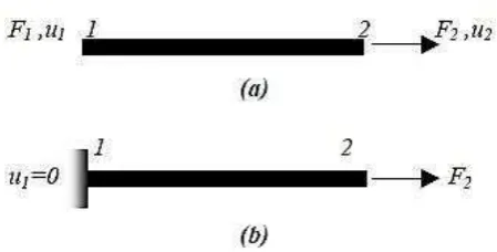
Each problem has natural or artificial boundary conditions. The boundary conditions provide a reference in which elastic displacements at various parts of the body can be measured. Consider a rod element (Figure 1.a). If a boundary condition is not defined for this element, it acts according to the large, small or equal forces of the acting node, and the rigid body movement is observed in the bar as displacement u1 = u2.
Figure 1. Console beam finite element model
The rigid body movement in the first case causes the overall resistance matrix to be singular. This can be attributed to the fact that a reference point to measure u1 and u2 is not specified. In fact, a reference point must be provided. When we think the same bar as in Figure 1.b;
U2 = F2 / k (1)
we can express. Because u1 = 0 is the limit condition of the bar. Thus, boundary conditions; it can be said that there are restrictions on the displacements of certain parts or parts of the body. These restrictions prevent the rigid displacement of the object and allow the external loads to be carried by the object. The same boundary conditions are defined for other vectors and scalar field problems where the finite element method is applied according to the type of the problem.
2.7 Solution of System Equation
For the solution, it is sufficient to reverse the resistance matrix by considering the boundary conditions of the system. However, in terms of computer capacity and computer time, the solution of very large matrices can be done with the Gauss elimination method and with less capacity and shorter time.
3.
Results and Discussion
The results obtained by the finite element method are different from the experimental results. This is usually due to the fact that people who design as users or programmers neglect some parameters. The finite element method calculates every parameter to be simulated and output to output.
4.
References
[1] Smith, W.F., 2001. Malzeme Bilimi ve Mühendisliği. Üçüncü basım. Çeviri Editörü, Nihat G. Kırıkoğlu, Literatür Yayınları, İstanbul, 724. [2] Lal, K.M., 1983.Low Velocity Transverse Impact Behavior of 8-Ply Graphite-Epoxy Laminates. Journal of Reinforced Plastics and Composites, 2, 216-225.
[3] Belingardi, G. and Vadori, R., 2002. Low Velocity Impact Tests of Laminate Glass Fiber-Epoxy Matrix Composite Material Plates. International Journal of Impact Engineering, 27, 213-229.
[4] Mitrevski, T., Marshall, I.H., Thomson, R., Jones, R. and Whittingham, B., 2004. The Effect of Impactor Shape on the Impact Response of Composite Laminates. Composite Structures, 67, 139-148.
[5] Rotem, A. and Lifshitz, J.M., 1971. Longitudinal Strength of Unidirectional Fibrous Composite under High Rate of Loading. Proc. 26th Annual Tech. Conf. Soc. Plastics Industry Reinforced Plastics, Composites Division, Washington, DC, Section 10-G: pp. 1-10.
[6] Whitney, J.M. and Pagano, N.J., 1970. Shear Deformation in Heterogeneous Anisotropic Plates. Journal of Applied Mechanics, 37, 1026-1031. [7] Gong, S.W. and Lam, K.Y., 1999. Transient Response of Stiffened Composite Plates Subjected to Low Velocity Impact. Composites, Part B, 30, 473-484.
[8] Kompozit Plakalarda Sıcaklığın Darbe Davranışına Etkisi. TÜBİTAK, Proje No; 104M426, İzmir, 6-8, 23-26.
[9] Lifshitz, J.M., 1976. Impact Strength of Angle Ply Fiber Reinforced Materials. Journal of Composite Materials, 10, 92-101.
[10] Abrate, S., 1998. Impact on Composite Structures. Cambridge University Press, Cambridge, 135-160.
[11] Cengiz, MS., Mamiş, MS., Yurci, Y. 2018. Providing electrical power increase by stimulating temperature difference at low temperatures in Stirling motors, Sigma Journal of Engineering and Natural Sciences, 36 (1), 87-97
[12] Cengiz, MS., Mamiş, MS., Kaynaklı M. 2017. The Temperature-Pressure-Frequency Relationship Between Electrical Power Generating in Stirling Engines, International Journal of Engineering
Research and Development, 9 (2)
[13] Cengiz, MS., Mamiş, MS., 2016. Analysis of Electrical Efficiency in Stirling Engine for Temperature Increase, International Workshop on Special Topics on Polymeric Composites, February 24, 2016.
[14] Çıbuk, M., Balık, H.H., (2010). A Novel Communication Application Model for Biomedical Networks, Fırat University Journal of Enginering, 22(1), 95-109.
[15] Efe, S.B. 2015. Artificial Neural Network Based Power Flow Analysis for Micro Grids, Bitlis Eren Univ J Sci & Technology, 5 (1), pp. 42-47.
[16] Baucom, J.N. and Zikry, M.A., 2005. Low Velocity Impact Damage Progression in Woven E-glass Composite Systems. Composites, 36, 658-664. [17] Sankar, B.V., 1992. Scaling of Low Velocity Impact for Symmetric Composite Laminates. Journal of Reinforced Plastics Composites, 11, 297-305. [18] Sierakowski, R.L. and Chaturvedi, S.K., 1997. Dynamic Loading and Characterization of Fiber-Reinforced Composites. New York, Wiley.
[19] Abatan, A., Hu, H. and Olowokere, D., 1998. Impact Resistance Modeling of Hybrid Laminated Composites. Journal of Thermoplastic Composite Materials, 11, 249-260.
[20] Sun, C.T. and Chattopadhyay, S., 1975. Dynamic Response of Anisotropic Laminated Plates under Initial Stress to Impact of a Mass. ASME Journal of Mechanics, 42, 693-698.