Time Domain and Frequency Domain Deterministic Channel
Modeling for Tunnel/Mining Environments
Chenming Zhou1, *, Ronald Jacksha2, Lincan Yan1, Miguel Reyes1, and Peter Kovalchik1
Abstract—Understanding wireless channels in complex mining environments is critical for designing optimized wireless systems operated in these environments. In this paper, we propose two physics-based, deterministic ultra-wideband (UWB) channel models for characterizing wireless channels in mining/tunnel environments — one in the time domain and the other in the frequency domain. For the time domain model, a general Channel Impulse Response (CIR) is derived and the result is expressed in the classic UWB tapped delay line model. The derived time domain channel model takes into account major propagation controlling factors including tunnel or entry dimensions, frequency, polarization, electrical properties of the four tunnel walls, and transmitter and receiver locations. For the frequency domain model, a complex channel transfer function is derived analytically. Based on the proposed physics-based deterministic channel models, channel parameters such as delay spread, multipath component number, and angular spread are analyzed. It is found that, despite the presence of heavy multipath, both channel delay spread and angular spread for tunnel environments are relatively smaller compared to that of typical indoor environments. The results and findings in this paper have application in the design and deployment of wireless systems in underground mining environments.†
1. INTRODUCTION
As mandated by the Mine Improvement and New Emergency Response Act (MINER Act) [2], wireless communication and tracking systems are required in all U.S. underground coal mines. To design reliable, high-performance wireless communication and tracking systems that can be deployed in highly complex mining environments, it is essential to understand the wireless channels in these environments.
Characterization of wireless channels in underground mines has been extensively investigated for decades [3–8]. Early research on characterizing underground mine environments mainly focused on measurement-based empirical methods [9]. Recently, statistically channel models that have been widely used to characterize wireless channels on the surface were applied to study underground mine channels [5, 6, 10–13]. Channel properties such as delay spread, power delay profile, and coherent bandwidth have been discussed based on statistical channels [14, 15].
While it is mathematically useful, a statistical channel model does not reveal the important connection between the channel and the physical world. It is known that, in principle, with the knowledge of electromagnetic boundary conditions (e.g., location, shape, and electrical properties of all objects in the environment), field strength (and thus signal power) at any point can be determined by numerically solving Maxwell’s equations. As a result, a wireless channel, theoretically, should be treated as deterministic. A deterministic channel model is attractive as it provides physical insight into how the channel properties are affected by the physical environment. For example, a physics-based
Received 29 August 2017, Accepted 3 November 2017, Scheduled 28 November 2017 * Corresponding author: Chenming Zhou ([email protected]).
1 National Institute for Occupational Safety and Health, Pittsburgh Mining Research Division, USA. 2 National Institute for Occupational Safety and Health, Spokane Mining Research Division, USA.
Ultra-wideband (UWB) channel model is proposed in [16] for characterizing UWB channels in urban environments with high-rise buildings. The model is based on time domain electromagnetics and takes into account environmental parameters such as the height of the buildings and the spacing between adjacent buildings. The model has been applied to characterize cylinder diffraction channels in [17]. In this paper, we will extend the work in [16] to underground channels and develop physics-based channel models for confined mining environments.
Underground mining environments generally consist of mine entries and cross cuts that are similar to a road or subway tunnel. As a result, tunnel propagation theory has been applied to analyze radio propagation in mines [3, 4] for decades. Ray tracing and modal methods are the two common methods for modeling radio propagation in tunnel environments. The ray tracing method treats radio waves as ray tubes that can be reflected by the four tunnel walls. Given a transmitter location, the received electrical field (or power) at any location within a tunnel is obtained by summing up the contributions of all the rays that reach the receiver. The ray tracing method has been widely used for predicting indoor wireless transmission [18], evaluating field distribution in tunnels [19, 20] as well as hallways [21], and predicting delay spread in tunnel environments [22]. Depending on the way those rays that reach the receiver are identified, the ray tracing method can be divided into two categories—image-based ray tracing and shoot and bouncing ray (SBR) tracing. The image-based ray tracing [4, 20] has a relatively low computation complexity, but its application is usually limited to environments with simple geometries. The SBR algorithm [23] can handle more complex environments (e.g., curved tunnels [24]) but requires significantly more computation resources and longer computation time.
For the modal method, tunnels are viewed as hollow dielectric waveguides, and analytical solutions of Maxwell’s wave equations are sought. It is found that while rigorous analytical solutions are available for circular tunnels [25], determining the exact solution for a rectangular waveguide is not mathematically possible due to the difficulty in matching boundary conditions. By only matching boundary conditions along the four surfaces of the dielectric waveguide and ignoring the mismatch in the corner regions of the dielectric, Laakmann and Steier obtained the approximate solutions for rectangular tunnels in [26] through studying hollow dielectric waveguide for optical applications. The same approximated modal solutions were found independently by Emslie et al. in [3] under a project sponsored by the U.S. Bureau of Mines (USBM).
Compared to existing literature [3–7, 14, 15], a unique contribution of this paper is that we connect the wireless community to the electromagnetic (EM) community by relating channel models that are widely used in the wireless community to waves and fields known in the electromagnetic community. We derived a general Channel Impulse Response (CIR) and complex channel transfer function for the wireless channels in tunnel environments based on the ray tracing and modal methods developed in the EM community, respectively. RF measurements were taken to validate the derived channel models. Channel properties such as delay spread, multipath component number, and angular spread are discussed and their connection to environment properties such as tunnel dimensions are investigated. 2. TIME DOMAIN UWB CHANNEL MODELING FOR TUNNEL ENVIRONMENTS 2.1. General Time Domain UWB Channel Model
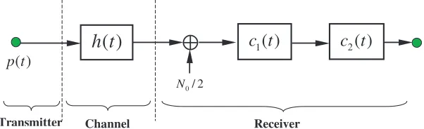
Figure 1 illustrates a general UWB communication system. In Fig. 1, p(t) is the transmitted pulse waveform, and h(t) represents the CIR. The received signal before the filterc1(t) can be written as
r(t) =p(t)∗h(t) +n(t) =y(t) +n(t), (1) wheren(t) is Additive White Gaussian Noise (AWGN) with a two-sided power spectral density ofN0/2.
It is known that, given y(t) =p(t)∗h(t), a matched filter — matched toy(t) — provides the maximum signal-to-noise power ratio (SNR) at its output. The matched filter can be virtually decomposed into two filters, with the first filterc1(t) matched to the CIRh(t) and the second filterc2(t) matched to the
pulse waveform p(t).
A general Wide Sense Stationary (WSS) UWB channel is often modeled as a tapped delay line [16, 27]:
h(t) =
L
l=1
0/ 2 N
1
( )
c t
c t
2( )
( )
p t
Receiver Channel
Transmitter
( )
h t
Figure 1. A general model for wireless data transmission.
whereL is the number of multipath components, andAl and τl are the amplitude and delay of the lth multipath component, respectively. In this case, the received signals are just a series of attenuated and time-shifted replicas of the transmitted pulse. It should be noted that the antenna, which is generally frequency selective, has not been included in the channel model shown in Eq. (2). Although some research has proposed including antennas as part of the channel for an optimum system design, in this paper we will only focus on channel modeling without considering the frequency selectivity of the transmitter and receiver antennas.
In practice, the estimation of CIR h(t) is generally a challenging task, especially when there is per-path pulse distortion for wide band signals [16]. It would be desirable if an analytical model for
h(t) were available. The analytical form of h(t) is useful for investigating system performance under different configurations (e.g., for studies that pertain to time reversal [28, 29]).
2.2. Time Domain UWB Channel Model for Tunnel Environments
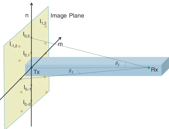
We consider a rectangular tunnel with its cross-sectional view depicted in Fig. 2. The origin of the coordinate system is oriented at the center of the tunnel, with x horizontal, y vertical, and z down the tunnel. Let 2a and 2b denote the width and height of the tunnel, respectively. According to the image-based ray tracing theory, the received signal at a given location within the tunnel can be obtained by summing up all the signals radiated from an image plane shown in Fig. 3. Each image on the image plane is a virtual signal source that can be represented by an equivalent antenna. As a result, the source is equivalent to a large antenna array with theoretically an infinite number of elements located on the image plane. For a transmitter located atT(x0, y0,0), the received signal at an arbitrary location
R(x, y, z) within the tunnel can be calculated as [4, 7, 20, 30]:
Ey
r(x, y, z) =Et +∞
m=−∞ +∞
n=−∞
e−jkrm,n
rm,n ρ |m|
⊥ ρ|n| (3)
where the superscript “y” denotes a vertically polarized source. Et is a constant determined by the transmitted power. k= 2π/λ is the free space wave vector and λ is the wavelength. The integers m and nare the orders of the image Im,n which represent the number of reflections that a ray undergoes
m n
Tx
Image Plane
Rx x
θ θy
I0,2
I0,1
I0,-1
I0,-2 I-1,2
I1,2
Figure 3. A diagram to show that multipath components in a rectangular can be represented by corresponding rays oriented from image sources (Im,n) on a virtual image plane perpendicular to the tunnel axis.
relative to the vertical and horizontal walls, respectively. The signs of m and n indicate whether the image is located on the positive or negative side of thexandy axis, respectively. Note that as a special case when m = n = 0, the image I0,0 becomes the point source itself and the ray path associated
with the image I0,0 becomes the well known line-of-sight (LOS) path. The path length rm,n and the
coordinate of the image Im,n are given by:
rm,n =
(xm−x)2+ (yn−y)2+z2
xm = 2ma+ (−1)mx0
yn= 2nb+ (−1)ny0
(4)
In Eq. (3), ρ⊥, are the Fresnel reflection coefficients for the perpendicular and parallel polarizations, respectively. Under grazing incidences, the Fresnel reflection coefficients can be approximated as [20]
ρ⊥, ≈ −exp
−2 cosθ ⊥,
Δ⊥,
(5) where the corresponding incident anglesθ⊥, and surface impedances Δ⊥, are given by:
θ⊥= 90−θx = acos
|xm−x|
rm,n
θ = 90−θy = acos
|yn−y|
rm,n
(6)
Δ≈ √
¯
εb−1
¯
εb
Δ⊥≈√ε¯a−1
(7)
where ¯εa,b = εa,b/ε0 are the complex relative permitivities for the horizontal and vertical walls,
normalized by the vacuum permitivityε0. ¯εa,b can be expressed as
¯
εa,b= ¯εra,b−j2σπfεa,b 0
where ¯εra,b denotes the real part of the relative permittivity ¯εa,b. σa,b are the conductivity of the horizontal and vertical walls, respectively. f is the frequency.
It is apparent from Eq. (3) that rays and images for the ray tracing method are determined by tunnel dimensions as well as Tx/Rx locations, but are independent of frequency. As far as propagation mechanisms are considered, diffraction from edges [16] or curved surfaces [17] often introduces frequency dependency (pulse distortion) but reflections from smooth surfaces generally have little frequency dependency. As a result, we expect that the result in Eq. (3) is independent of frequency except for the term −jkrm,n which is caused by the retarded time. Therefore, the ray tracing method can be considered as a time domain method.
Mathematically, if the frequencyf is sufficiently high such that σa,b/(2πfε¯ra,bε0) 1 is satisfied,
tunnel walls generally act as a good dielectric where the displacement current density is much greater than the conduction current density [20]. As a result, the imaginary term in Eq. (8) can be ignored and thus the relative permitivity ¯εa,b ≈ε¯ra,b can be viewed as being independent of frequency.
Assuming that the frequency is high and applying the Inverse Fast Fourier Transform (IFFT) to Eq. (3), the corresponding time domain CIR can be expressed in the classic tapped delay line model as
hy(t) = +∞ n=−∞
+∞
m=−∞
Ay
m,nδ(t−τm,n) (9)
where
Ay
m,n = (−1) (m+n)
rm,n exp
−2
rm,n
|√xm−x|
¯
εr a−1 +
|yn−y|ε¯rb
¯
εr b −1
,
τm,n = rm,nc
(10)
In Eq. (10), c is the speed of light in vacuum and the superscript y denotes y-polarization (vertical polarization).
Similarly, the corresponding time domain CIR forx-polarized (horizontally polarized) signals can be expressed as
hx(t) = +∞ n=−∞
+∞
m=−∞
Ax
m,nδ(t−τm,n) (11)
where
Axm,n = (−1)
(m+n)
rm,n exp
−2
rm,n
|x√m−x|ε¯ra
¯
εra−1 +
|yn−y|
¯
εr b−1
(12) With the derived CIR given in Eqs. (9) and (10), the received signal r(t) can be conveniently obtained by convolving the transmitted pulsep(t) with the CIR based on Eq. (1). It is shown in Eqs. (9) and (10) that the proposed physics-based CIR for tunnel/mining environments takes the following environmental and system factors into account:
• Transmitter location: (x0, y0, z0)
• Receiver location: (x, y, z) • Source polarization
• Dimensions of the tunnel (2a,2b)
• Electric properties of the tunnel walls (¯εra,ε¯rb)
It is interesting to note that upon fixing all the five factors above, CIRs for tunnel environments are deterministic and do not vary with time. NIOSH researchers have recently experimentally proven the time invariance of wireless channels for tunnel environments by showing that power measurement results taken on different dates in a train tunnel remained the same [31].
2.3. Metrics for Characterizing Wireless Channels
2.3.1. Multipath Component Number
To design an optimal communication system, multipath richness of the communication channel needs to be taken into consideration. The presence of a large number of multipath components often leads to multipath fading — an issue that has been combated in the wireless community for decades. On the other hand, advanced wireless techniques such as Multiple-Input Multiple-Output (MIMO) and Time Reversal (TR) [28] might actually take advantage of the richness of multipath to improve system throughput and communication range.
It is generally challenging to determine the exact multipath components of a wireless channel unless the channel is extremely simple, as in the case for a two-ray model. Practically, advanced algorithms such as the CLEAN algorithm [28, 32] are often used to extract the CIR (and thus multipath components) from received wideband signals based on deconvolution operations.
Theoretically, as shown in Eqs. (9) and (11), an infinite number of multipath components exist as radio waves propagate in a confined tunnel environment. Practically, however, only a limited number of multipath components make a noticeable contribution to the received signal and need to be included in the model. As a result, we can limit the range of the indexmand nin (9) to [−M, M] and [−N, N], respectively. Given the numbers ofM andN, the number of the multipath components can be calculated as
NMP = (2M+ 1)(2N + 1) (13)
As a special case, for M =N = 0, only the LOS path is included in the model, so Eqs. (9) and (11) are reduced to the free space propagation case where the standard Friis transmission equation can be applied.
2.3.2. Delay Spread
Another important metric for characterizing the multipath richness of wireless communication channels is the delay spread. Root Mean Square (RMS) delay spread is widely used to describe the time dispersion property of the channel and is closely related to the Inter Symbol Interference (ISI) of a communication system. A channel with a small RMS delay spread generally allows a wireless system to transmit signals faster without performance degradation caused by ISI. The corresponding metric in the frequency domain is the coherence bandwidth, which is the bandwidth over which the channel can be assumed flat.
With the derived analytical CIR, the RMS delay spread of the channel at a given distance can be readily computed as [28, 33]:
τrmsx,y =
+∞
n=−∞ +∞
m=−∞
(τm,n−τ¯)2Ax,ym,n2
+∞
n=−∞ +∞
m=−∞
Ax,y
m,n2
(14)
where the mean delay ¯τ is defined as
¯
τ =
+∞
n=−∞ +∞
m=−∞
τm,nAx,ym,n2
+∞
n=−∞ +∞
m=−∞
Ax,y
m,n2
(15)
2.3.3. Angular Spread
(DoD) and the direction of arrival (DoA) [27]. Channel directional properties are particularly important in the context of multi-antenna systems.
According to the original ray representation of the electrical field shown in Eq. (3), the DoA and DoD for the (m, n) ray (path) are about the same and can be approximated by
θx(m)≈ |xm−x|
(xm−x)2+z2
θy(n)≈ |yn−x| (yn−y)2+z2
(16)
where θx,y are the angular spread in the x and y dimensions, respectively. An example of θx,y is illustrated in Fig. 3, where mulipath components are represented by the corresponding rays oriented from a series of image sources on a virtual image plane. For example, the LOS path is represented by the line connecting the source I0,0 and the receiver Rx. It has been assumed in Eq. (16) that the
receiver is sufficiently far from the transmitter such thatz |xm−x|and z |yn−x|are satisfied for all the images included in the model.
3. FREQUENCY DOMAIN CHANNEL MODELING FOR TUNNEL ENVIRONMENTS
Based on the modal method given in [30], the complex channel transfer function can be expressed as
H(f) = −j2π
ab · +∞ p=1 +∞ q=1
Bp,qe
−[αp,q(f)+jβp,q(f)]z
βp,q(f) (17) where
Bp,q= sin
pπ
2ax+ ¯ϕp
sin
qπ
2by+ ¯ϕq
×sin
pπ
2ax0+ ¯ϕp
sin
qπ
2by0+ ¯ϕq
,
αp,q(f) =1
b qc 4bf 2 Re 1 √ ¯
εb−1
+1 a pc 4af 2 Re ¯ εa √ ¯
εa−1
βp,q(f) =
(2πf
c )2−
pπ
2a
2
−qπ 2b
2
(18)
ϕp,q=
0 p(q) is even
π/2 p(q) is odd (19)
The received signal in the frequency domain can be obtained by multiplying the frequency spectrum of the transmitted pulseP(f) with the complex channel transfer functionH(f) as:
R(f) =P(f)H(f) (20) Similar to the image ordersm, nfor the time domain method, the mode ordersp, qfor the frequency domain method need to be limited to finite numbersP, Q for practical implementations.
4. MEASUREMENT
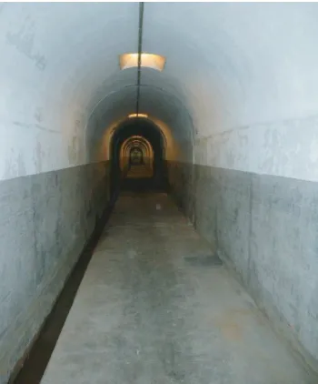
Figure 4. A picture of the concrete tunnel where propagation measurements were taken.
5. RESULTS AND DISCUSSION
Simulations were performed to analyze wireless channels in tunnel environments in both the time and the frequency domains. Measurement results taken in the concrete tunnel introduced in Section 4 will be used to validate the simulation results. Unless stated otherwise, parameters used in the simulations are listed in Table 1. In our simulation, the arched tunnel shown in Fig. 4 has been approximated by a rectangular tunnel with the same width (1.83 m) and an equivalent height of 2.35 m. The equivalent height, along with the electrical parameters (i.e., the conductivity and relative dielectric constant) of the tunnel, were optimized based on minimizing the difference between the simulated and measured results. The other parameters in Table 1 are chosen based on the parameters used in real measurements. For example, the coordinates of the transmitter and receiver antennas, i.e., (x0, y0) and (x, y), are chosen
based on the fact that both antennas were placed in the center of the tunnel with an antenna height of 1.22 m.
Table 1. A list of the parameters used in the simulations.
Parameter Value Parameter Value
2a 1.83 m 2b 2.35 m
x0 0 x 0
y0 0.0457 m y 0.0457 m
¯
εr
a,b 8.9
5.1. Time Domain Channel Characteristics
5.1.1. Multipath Components
-2 0 2 4 -5
0
5
z = 6 m
n
m
-40 -20 0 20 40
-40
-30
-20
-10
0
10
20
30
40
z = 6 00 m
n
m
(a) (b)
Figure 5. A heat map for visualizing the contribution of each multipath component (image) on the image plane. Each rectangular block (pixel) represents one image (Im,n) on the image plane with its intensity represented by the block color. (a) z= 6 m. (b) z= 600 m.
the LOS signal that always has the least attenuation caused by the channel. As a result, the center of the image plane is always red (maximum value). The intensities of each virtual signal source in Fig. 5 have been normalized with respect toA0,0 for a better visualization effect.
It is found from Fig. 5(a) that for a short separation distance (z = 6 m) only a small number of images (m < 3, n < 2) make noticeable contributions to the received signal. As we recall that the signal source for a receiver within a tunnel can be viewed as a large antenna array placed on the image plane, the receiver “sees” a relatively small array for this case when the separation distance is short. As shown in Fig. 5(b), however, the element number and thus the physical size of the “antenna array” significantly increase with the separation distance. The results in Fig. 5 are simulated based on a specific case where the frequency is set as 455 MHz and the polarization is vertical. The finding, however, is general to all other frequencies and polarizations. Another interesting observation from Fig. 5(b) is that the equivalent antenna array appears to be an ellipse for a rectangular tunnel. This is due to the fact that signals radiated from images in the corner of the image plane generally go through more reflections before they reach the receiver and thus are attenuated more compared to signals radiated from images
0 100 200 300 400 500 600 0
5 10 15 20
Distance (m)
Max Index
N(z)
M(z)
close to the X or Y axis on the image plane. Generally, the intensity of images decreases with the product of m and n which explains why the brightest point occurs in the center of the heat map and then the brightness gradually decreases toward the edge of the image plane.
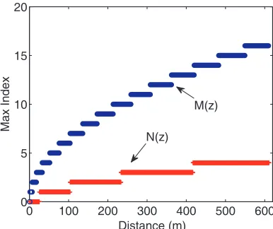
Figure 6 shows the maximum index of the images/rays (defined as rays that are 20 dB lower in power than the LOS signals) for different separation distancesz. M(z) andN(z) represent the corresponding maximum image index for the horizontal and vertical dimensions, respectively. It is straightforward that the maximum index increases with separation distance for both horizontal and vertical dimensions. For small distances (z < 10 m), the maximum order is zero which means only LOS is needed. For a given separation distance, the horizontal (X) dimension requires more images than the vertical (Y) dimensions which is consistent with what is shown in Fig. 5. For example, at the distance of 600 meters, the maximum order of horizontal and vertical images are 16 and 4, respectively. As a result, a total number of 297 multipath components need to be considered for this case. It should be noted that the value of M(z) and N(z) are dependent on several factors including tunnel dimensions, source polarization, and reflectivity of the surface on each dimension.
5.1.2. Channel Impulse Response
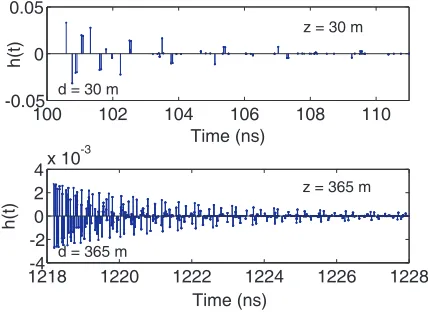
Figure 7 shows two examples (corresponding to two separation distances of 30 m and 365 m, respectively) of the simulated CIRs in the tunnel. CIRs are calculated based on the tapped delay line model given by Eq. (11). It is apparent from Fig. 7 that the number of noticeable multipath components increases with the separation distance. The analytical model given in Eq. (11) would be useful for system design since joint optimization of wireless communication and networked control systems often requires full knowledge of CIR or channel transfer function.
100 102 104 106 108 110
-0.05 0 0.05
Time (ns)
h(t)
d = 30 m
1218 1220 1222 1224 1226 1228
-4 -2 0 2 4x 10
-3
Time (ns)
h(t)
d = 365 m
z = 30 m
z = 365 m
Figure 7. Simulated CIRs in a tunnel environ-ment at different transmitter-receiver separation distances.
0 100 200 300 400 500 600
1.4 1.5 1.6 1.7
Distance (m)
RMS Delay Spread (ns)
Figure 8. Simulated RMS delay spreads at different transmitter-receiver separation d distances.
5.1.3. Delay Spread
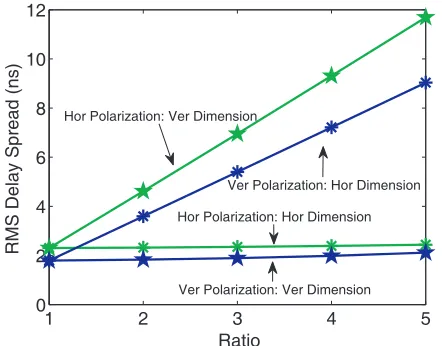
One possible explanation for the smaller RMS delay spread in Fig. 8 is that the transversal dimensions of the tunnel used in the simulation are smaller as compared to typical indoor office environments. We thus investigated how RMS delay spreads vary with tunnel dimensions, and the corresponding simulation results are shown in Fig. 9. The horizontal axis of the Fig. 9 is the ratio of the transverse dimensions with respect to the original dimensions given in Table 1. For each of the four simulation curves shown Fig. 9, only one of the transverse dimensions (either the x or y dimension) varies and the other remains the same. It is found that, depending on the source polarization, the RMS delay spread linearly increases with one of the transverse dimensions but remains relatively stable with the change of the other dimension. For example, for a horizontally polarized signal source (the two green curves in Fig. 9), the RMS delay spread increases linearly with the vertical dimension (height) of the tunnel and almost remains unchanged as the horizontal dimension (width) of the tunnel varies.
1 2 3 4 5
0 2 4 6 8 10 12
Ratio
RMS Delay Spread (ns)
Hor Polarization: Hor Dimension Hor Polarization: Ver Dimension
Ver Polarization: Hor Dimension
Ver Polarization: Ver Dimension
Figure 9. RMS delay spread varies with the dimensions of the tunnel and the polarization of the signal source.
0 100 200 300 400 500 600
0 10 20 30 40 50
Distance (m)
Max Angle (Deg)
max( y) max( x)
θ θ
Figure 10. Maximum spread angle varies with the separation distance.
5.1.4. Angular Spread
For a deterministic model, each multipath component has a deterministic angular spread in both thex and ydimensions. The corresponding angular spreads for each multipath component can be calculated based on Eq. (16). Fig. 10 shows the maximum angular spreads among all of the significant multipath components for different distances along the axis of the tunnel, for both x and y dimensions. It is found that the maximum angular spread decreases with distance for both dimensions. It is also shown in Fig. 10 that the angular spreads in the far zone (e.g., for z > 100 m) could be as small as a few degrees. Small angular spreads for tunnel environments can be explained by the fact that signals are well confined in the tunnel and thus would not spread as much as they would in an open environment. Small angular spread in tunnel environments suggests that different antenna patterns probably would not change the overall profile of the propagation behavior in the tunnel except for introducing a constant gain when the receiver is located far from the transmitter.
5.2. Channel Transfer Function
1 2 3 4 5 -400
-300 -200 -100 0
Frequency (GHz)
|H(f)| (dB)
Frequency domain method Time domain method
Figure 11. An example of simulated channel transfer function |H(f)| for tunnel environments when the transmitter and the receiver are separated far from each other (z= 500 m).
1 2 3 4 5
-50 -40 -30 -20 -10 0
Frequency (GHz)
|H(f)| (dB)
Frequency domain method Time domain method
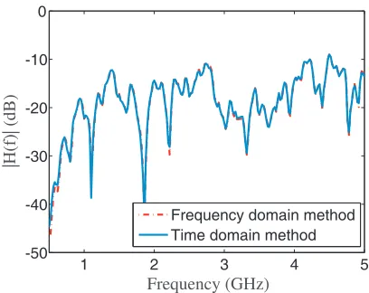
Figure 12. An example of simulated channel transfer function |H(f)| for tunnel environments when the transmitter and the receiver are close to each other (z = 50 m). The channel transfer function obtained by applying the IFFT to the time domain CIR is also plotted for reference.
It should be noted that UWB channel transfer functions for indoor environments can be measured through S21 parameters by a Vector Network Analyzer (VNA). VNAs have been recently used to
measure wireless channels for tunnel environments such as road tunnels [38], hallways [39], and mine entries [10, 12]. A comparison of our simulated transfer function and measured ones (e.g., the one shown in [39] for hallway environments) shows that both have periodical nulls and peaks which are caused by interference from multiple modes. The reason why nulls and peaks are not noticeable in Fig. 11 for frequencies below 2 GHz is due to higher-order modes for low-frequency signals which are significantly attenuated at 500 m and thus will not interfere with the dominant mode. In other words, the smooth curve associated with the section for frequencies below 2 GHz in Fig. 11 is an indication of the single-mode propagation scenario. When the Tx and Rx are relatively close to each other (Fig. 12), it is observed that low frequency signals do not show significantly lower loss compared to high frequency signals as shown in Fig. 11. It is apparent from Fig. 11 that high frequency signals are more favorable for tunnel environments in terms of the propagation loss, without considering the loss caused by the transmitter and receiver antennas. However, high frequency signals often have higher loss caused by the radiating elements — antennas. Both the antenna loss and the propagation loss should be considered when the optimum frequency for tunnel environments is desired [35].
5.3. Power Attenuation along Tunnel Axial Distance
0 100 200 300 400 500 600 -140
-120 -100 -80 -60 -40 -20
Distance (m)
Received Power (dBm)
f = 915 MHz
Measurement M=N=0, LOS only
M=N=20
M=N=40
Figure 13. A comparison between the simulated (based on the derived CIR) and measured signal power attenuation at 915 MHz in the concrete tunnel.
0 100 200 300 400 500 600 -120
-110 -100 -90 -80 -70 -60 -50 -40 -30
Distance (m)
Received Power (dBm)
f = 5800 MHz
Measurement
Simulation: Time domain Simulation: Frequency domain
Figure 14. A comparison between the simulated and measured power attenuation at 5.8 GHz in the concrete tunnel.
image orders M and N increase. Additionally, it is found that larger values of M and N are needed for greater distances in order to include all the significant multipath components. For example, it is shown in Fig. 13 that M =N = 20 is sufficient for including all the major multipath components for any distances less than 345 m, but is not sufficient for distances greater than 345 m. This is consistent with the observation from Figs. 5 and 6. Another interesting finding is that when the receiver is located in the vicinity of the transmitter, only the LOS path needs to be considered in the model, as evidenced by the fact that the M = N = 0 curve already shows a good agreement with the measurement curve for short separation distances. This is consistent with the result shown in Fig. 5(a).
Figure 14 shows a comparison between the measured and simulated received signal power at 5.8 GHz for the same tunnel. M =N = 40 is used in the time domain impulse response andP =Q= 5 is used for the frequency domain channel transfer function. It is shown that the time domain simulated result matches the frequency simulation result well and that both simulated results agree reasonably with the measurement result.
6. CONCLUSION
ACKNOWLEDGMENT
The authors would like to thank Mr. Timothy Plass for his help with collecting the measurement data. The authors also thank Dr. Joseph Waynert, Mr. Alan Mayton, and Mr. Joe Schall for reviewing the manuscript.
REFERENCES
1. Zhou, C., “Physics-based ultra-wideband channel modeling for tunnel/mining environments,”2015
IEEE Radio and Wireless Symposium (RWS), 92–94, Jan. 2015.
2. “The mine improvement and new emergency response act of 2006 (MINER Act),” Jun. 2006, [Online], Available: http://www.msha.gov/MinerAct/MinerActSingleSource.asp.
3. Emslie, A., R. Lagace, and P. Strong, “Theory of the propagation of UHF radio waves in coal mine tunnels,”IEEE Transactions on Antennas and Propagation, Vol. 23, No. 2, 192–205, 1975.
4. Mahmoud, S. and J. Wait, “Geometrical optical approach for electromagnetic wave propagation in rectangular mine tunnels,” Radio Science, Vol. 9, No. 12, 1147–1158, 1974.
5. Li´enard, M. and P. Degauque, “Natural wave propagation in mine environments,” IEEE
Transactions on Antennas and Propagation, Vol. 48, No. 9, 1326–1339, 2000.
6. Zhang, Y. P., G. X. Zheng, and J. Sheng, “Radio propagation at 900 MHz in underground coal mines,”IEEE Transactions on Antennas and Propagation, Vol. 49, No. 5, 757–762, 2001.
7. Sun, Z. and I. F. Akyildiz, “Channel modeling and analysis for wireless networks in underground mines and road tunnels,”IEEE Transactions on Communications, Vol. 58, No. 6, 1758–1768, 2010. 8. Zhou, C., “Ray tracing and modal methods for modeling radio propagation in tunnels with rough
walls,”IEEE Transactions on Antennas and Propagation, Vol. 65, No. 5, 2624–2634, 2017.
9. Goddard, A. E., “Radio propagation measurements in coal mines at UHF and VHF,” Proc.
Through-Earth Electromagn., 15–17, 1973.
10. Boutin, M., A. Benzakour, C. L. Despins, and S. Affes, “Radio wave characterization and modeling in underground mine tunnels,”IEEE Transactions on Antennas and Propagation, Vol. 56, No. 2, 540–549, 2008.
11. Boutin, M., S. Affes, C. Despins, and T. Denidni, “Statistical modelling of a radio propagation channel in an underground mine at 2.4 and 5.8 GHz,”IEEE 61st Vehicular Technology Conference,
VTC 2005-Spring, Vol. 1, 78–81, 2005.
12. Nerguizian, C., C. L. Despins, S. Aff`es, and M. Djadel, “Radio channel characterization of an underground mine at 2.4 GHz,” IEEE Transactions on Wireless Communications, Vol. 4, No. 5, 2441–2453, 2005.
13. Qaraqe, K. A., S. Yarkan, S. G¨uzelg¨oz, and H. Arslan, “Statistical wireless channel propagation characteristics in underground mines at 900 MHz: A comparative analysis with indoor channels,”
Ad Hoc Networks, Vol. 11, No. 4, 1472–1483, 2013.
14. Yarkan, S. and H. Arslan, “Statistical wireless channel propagation characteristics in underground mines at 900 MHz,”IEEE Military Communications Conference (MILCOM07), 1–7, IEEE, 2007. 15. Chehri, A., P. Fortier, and P. M. Tardif, “Large-scale fading and time dispersion parameters
of UWB channel in underground mines,” International Journal of Antennas and Propagation, Vol. 2008, 2008.
16. Qiu, R. C., C. Zhou, and Q. Liu, “Physics-based pulse distortion for ultra-wideband signals,”IEEE
Transactions on Vehicular Technology, Vol. 54, No. 5, 1546–1555, 2005.
17. Zhou, C. and R. C. Qiu, “Pulse distortion caused by cylinder diffraction and its impact on uwb communications,”IEEE Transactions on Vehicular Technology, Vol. 56, No. 4, 2385–2391, 2007. 18. Valenzuela, R. A., “A ray tracing approach to predicting indoor wireless transmission,” IEEE
Vehicular Technology Conference, 214–218, 1993.
20. Zhou, C., J. Waynert, T. Plass, and R. Jacksha, “Attenuation constants of radio waves in lossy-walled rectangular waveguides,” Progress In Electromagnetics Research, Vol. 142, 75–105, 2013. 21. Porrat, D. and D. C. Cox, “UHF propagation in indoor hallways,”IEEE Transactions on Wireless
Communications, Vol. 3, No. 4, 1188–1198, 2004.
22. Kermani, M. H. and M. Kamarei, “A ray-tracing method for predicting delay spread in tunnel environments,” IEEE International Conference on Personal Wireless Communications, 538–542, 2000.
23. Chen, S.-H. and S.-K. Jeng, “SBR image approach for radio wave propagation in tunnels with and without traffic,” IEEE Transactions on Vehicular Technology, Vol. 45, No. 3, 570–578, 1996. 24. Wang, T.-S. and C.-F. Yang, “Simulations and measurements of wave propagations in curved road
tunnels for signals from gsm base stations,” IEEE Transactions on Antennas and Propagation, Vol. 54, No. 9, 2577–2584, 2006.
25. Marcatili, E. and R. Schmeltzer, “Hollow metallic and dielectric waveguides for long distance optical transmission and lasers,”Bell System Technical Journal, Vol. 43, No. 4, 1783–1809, 1964.
26. Laakmann, K. D. and W. H. Steier, “Waveguides: Characteristic modes of hollow rectangular dielectric waveguides,”Applied Optics, Vol. 15, No. 5, 1334–1340, 1976.
27. Molisch, A. F., Wireless Communications, John Wiley Sons, 2010.
28. Zhou, C., N. Guo, and R. C. Qiu, “Time-reversed ultra-wideband (UWB) multiple input multiple output (MIMO) based on measured spatial channels,”IEEE Transactions on Vehicular Technology, Vol. 58, No. 6, 2884–2898, 2009.
29. Garcia-Pardo, C., M. Lienard, P. Degauque, J.-M. Molina-Garcia-Pardo, and L. Juan-Ll´acer, “Experimental investigation on channel characteristics in tunnel environment for time reversal ultra wide band techniques,” Radio Science, Vol. 47, No. 1, 2012.
30. Zhou, C. and J. Waynert, “The equivalence of the ray tracing and modal methods for modeling radio propagation in tunnels,”IEEE Antennas and Wireless Propagation Letters, Vol. 13, 615–618, 2013.
31. Zhou, C. and R. Jacksha, “Modeling and measurement of radio propagation in tunnel environments,”IEEE Antennas and Wireless Propagation Letters, Vol. 16, 141–144, 2016.
32. Cramer, R., R. Scholtz, M. Z. Win, et al., “Evaluation of an ultra-wide-band propagation channel,”
IEEE Transactions on Antennas and Propagation, Vol. 50, No. 5, 561–570, 2002.
33. Rappaport, T. S., Wireless Communications: Principles and Practice, Prentice Hall PTR New Jersey, 1996.
34. Dudley, D., M. Lienard, S. Mahmoud, and P. Degauque, “Wireless propagation in tunnels,”IEEE
Antennas and Propagation Magazine, Vol. 49, No. 2, 11–26, Apr. 2007.
35. Zhou, C., T. Plass, R. Jacksha, and J. Waynert, “Measurement of RF propagation in mines and tunnels,”IEEE Antennas and Propagation Magazine, Vol. 57, No. 4, 88–102, 2014.
36. Plass, T., R. Jacksha, J. Waynert, and C. Zhou, “Measurement of RF propagation in tunnels,”
IEEE International Symposium on Antennas and Propagation (APS2013), Orlando, FL, USA,
Jul. 2013, 1604–1605.
37. Molisch, A. F., D. Cassioli, C.-C. Chong, S. Emami, A. Fort, B. Kannan, J. Karedal, J. Kunisch, H. G. Schantz, K. Siwiak, et al., “A comprehensive standardized model for ultrawideband propagation channels,” IEEE Transactions on Antennas and Propagation, Vol. 54, No. 11, 3151– 3166, 2006.
38. Molina-Garc´ıa-Pardo, J.-M., M. Lienard, P. Degauque, C. Garc´ıa-Pardo, and L. Juan-Ll´acer, “MIMO channel capacity with polarization diversity in arched tunnels,” IEEE Antennas and
Wireless Propagation Letters, Vol. 8, 1186–1189, 2009.
39. Sood, N., L. Liang, S. V. Hum, and C. D. Sarris, “Ray-tracing based modeling of ultra-wideband pulse propagation in railway tunnels,”IEEE International Symposium on Antennas and