FRACTIONAL RECTANGULAR CAVITY RESONATOR
H. Maab† and Q. A. Naqvi
Department of Electronics Quaid-i-Azam University Islamabad, Pakistan
Abstract—Fractional curl operator has been used to derive solutions to the Maxwell equations for fractional rectangular cavity resonator. These solutions to the Maxwell equations may be regarded as fractional dual solutions. Behavior of field lines and surface current density in fractional cavity resonator have been investigated with respect to the fractional parameter. Fractional parameter describes the order of fractional curl operator.
1. INTRODUCTION
Ten years before, interest in exploring the roles and applications of fractional calculus [1] and fractional operators in electromagnetics led to fractionalization of curl operator, an operator which is commonly used in electromagnetics. It is represented by curlα = (∇×)α and is known as fractional curl operator [2]. Generally, the parameter α is noninteger. For α = 0, the fractional curl operator becomes an identity operator. Whereas, the fractional curl operator transforms to conventional curl operator when α = 1. When α ranges between 0 and 1, the fractional curl operator behaves as intermediate operator between identity operator and conventional/ordinary curl operator.
According to the following relations [2]
Ef d =
(ik)−1∇×
α
E
ηHf d =
(ik)−1∇×αηH
the fractional curl operator generates the fractional dual solution (Ef d, ηHf d) to the Maxwell equations. In above equations E and H
are electric and magnetic fields respectively. Quantities k and η are the wavenumber and impedance of the medium. Forα= 0, the above relations yield solution (E, ηH) while for α = 1, above relations yield solution (ηH,−E). When α ranges between 0 and 1, above relations yield solutions which may be regarded as intermediate step between solution (E, ηH) and solution (ηH,−E). That is, intermediate between original solution to Maxwell equations and dual to the original solution to Maxwell equations.
Fractional curl operator has been applied by Naqvi and co-workers on variety of problems, e.g., fractional curl operator in chiral and bi-anisotropic medium, fractional dual solutions in metamaterials, fractional perfect electromagnetic structures, fractional waveguides and transmission lines etc. [3–15]. Valuable contributions on this topic are given by other authors [16–23].
In this paper, we have investigated fractional rectangular cavity resonator. Fractional fields and fractional surface current density in fractional rectangular cavity resonator has been studies.
2. FIELDS IN FRACTIONAL CAVITY RESONATOR
Consider a rectangular cavity resonator, constructed from a waveguide of rectangular cross-section having width aand height b(a≥b). The waveguide is closed by two perfectly conducting plates located atz= 0 and z=d(d≥a), forming a rectangular parallelepiped or rectangular cavity. Since both TM and TE modes can exist in a rectangular waveguide, we expect TM and TE modes in a rectangular cavity resonator too. For simplicity we choose the z-axis as the reference “direction of propagation”. Actually, the existence of conducting walls atz= 0 andz=dgive rise to multiple reflections and set up standing waves. Therefore, no wave propagates in an enclosed cavity. Note that the longitudinal variation for wave traveling in the +z-direction and−z-direction are described by propagation factorse−ikzz andeikzz
respectively. Consider the TMmnp mode in the rectangular cavity resonator. Where the three symbol{mnp} subscript designate a TM or TE standing wave pattern in cavity resonator. Field expressions are [24]
ˆ
zEz(x, y, z) = ˆzAmnpsin(kxx) sin(kyy) cos(kzz) (1a)
ˆ
xEx(x, y, z) = −xˆ kzkx
k2 c
Amnpcos(kxx) sin(kyy) sin(kzz) (1b)
ˆ
yEy(x, y, z) = −yˆ kzky
k2 c
ˆ
xηHx(x, y, z) = ˆx ikky
k2 c
Amnpsin(kxx) cos(kyy) cos(kzz) (1d)
ˆ
yηHy(x, y, z) =−yˆ ikkx
k2 c
Amnpcos(kxx) sin(kyy) cos(kzz) (1e)
wherekx= mπa ,ky = nπb and kz= pπd,m=n=p= 0,1,2. . .and
kc=
k2−k2
x−k2y−k2z.
We may develop TMmnp in cavity resonator as the linear combination of +z-direction and−z-direction traveling TM rectangular waveguide mode, and is given by
ˆ
zEz+(x, y, z) = ˆzAmn
2 sin(kxx) sin(kyy) exp(−ikzz) (2a) ˆ
xEx+(x, y, z) = −xˆikzkx 2k2
c
Amncos(kxx) sin(kyy) exp(−ikzz) (2b) ˆ
yEy+(x, y, z) = −yˆikzky 2k2
c
Amnsin(kxx) cos(kyy) exp(−ikzz) (2c) ˆ
xηHx+(x, y, z) = ˆxikky 2k2
c
Amnsin(kxx) cos(kyy) exp(−ikzz) (2d) ˆ
yηHy+(x, y, z) = −yˆikkx 2k2
c
Amncos(kxx) sin(kyy) exp(−ikzz) (2e) and
ˆ
zEz−(x, y, z) = ˆzAmn
2 sin(kxx) sin(kyy) exp(ikzz) (3a)
ˆ
xEx−(x, y, z) = ˆxikzkx 2k2
c
Amncos(kxx) sin(kyy) exp(ikzz) (3b)
ˆ
yEy−(x, y, z) = ˆyikzky 2k2
c
Amnsin(kxx) cos(kyy) exp(ikzz) (3c)
ˆ
xηHx−(x, y, z) = ˆxikky 2k2
c
Amnsin(kxx) cos(kyy) exp(ikzz) (3d)
ˆ
yηHy−(x, y, z) = −yˆikkx 2k2
c
Amncos(kxx) sin(kyy) exp(ikzz) (3e)
For +z-directed wave, the corresponding fractional field (E+f d, ηH+f d) are given by [using (11a) and (11b) in 2] are
E+f d = ˆxExf d+ + ˆyEyf d+ + ˆzEzf d+ (4a)
where
Exf d+ =−iAmn 2k2
c
kzkxcos
απ 2
+kkysin
απ 2 ×cos
kxx−α π 2
sin
kyy−α π 2
exp (−ikzz) (5a)
Eyf d+ =−iAmn 2k2
c
kzkycos
απ 2
−kkxsin
απ 2 ×sin
kxx−α π 2
cos
kyy−α π 2
exp (−ikzz) (5b)
Ezf d+ =Amn 2 cos απ 2 sin
kxx−α π 2
sin
kyy−α π 2
exp (−ikzz) (5c) and
ηHxf d+ = iAmn 2k2
c
kkycos
απ 2
−kzkxsin
απ 2 ×sin
kxx−α π 2
cos
kyy−α π 2
exp (−ikzz) (5d) ηHyf d+ = −iAmn
2k2 c
kkxcos
απ 2
+kzkysin
απ 2 ×cos
kxx−α π 2
sin
kyy−α π 2
exp (−ikzz) (5e) ηHzf d+ = −Amn
2 sin απ 2 cos
kxx−α π 2
cos
kyy−α π 2
exp(−ikzz) (5f)
Similarly, for −z-directed wave, the corresponding fractional field (E−f d, ηH−f d) becomes
E−f d = ˆxExf d− + ˆyEyf d− + ˆzEzf d− (6a)
ηH−f d = ˆxηHxf d− + ˆyηHyf d− + ˆzηHzf d− (6b)
where
Exf d− =−iAmn 2k2
c
−kzkxcos
απ 2
+kkysin
απ 2 ×cos
kxx−α π 2
sin
kyy−α π 2
exp (ikzz) (7a)
Eyf d− =−iAmn 2k2
c
−kzkycos
απ 2
−kkxsin
απ 2 ×sin
kxx−α π 2
cos
kyy−α π 2
Ezf d− = Amn 2 cos απ 2 sin
kxx−α π 2
sin
kyy−α π 2
exp (ikzz)
(7c) and
ηHxf d− = iAmn 2k2
c
kkycos
απ 2
+kzkxsin
απ 2 ×sin
kxx−α π 2
cos
kyy−α π 2
exp (ikzz) (7d)
ηHyf d− = −iAmn 2k2
c
kkxcos
απ 2
−kzkysin
απ 2 ×cos
kxx−α π 2
sin
kyy−α π 2
exp (ikzz) (7e)
ηHzf d− = −Amn 2 sin απ 2 cos
kxx−α π 2
cos
kyy−α π 2
exp (ikzz)
(7f)
The total fractional dual solution of TMmnpmode in the fractional rectangular cavity resonator becomes
Ef d = ˆxExf d+ ˆyEyf d+ ˆzEzf d (8a) ηHf d = ˆxηHxf d+ ˆyηHyf d+ ˆzηHzf d (8b)
where
Exf d = Exf d+ +Exf d− (9a)
Eyf d = Eyf d+ +Eyf d− (9b)
Ezf d = Ezf d+ +Ezf d− (9c)
ηHxf d = ηHxf d+ +ηHxf d− (9d)
ηHyf d = ηHyf d+ +ηHyf d− (9e)
ηHzf d = ηHzf d+ +ηHzf d− (9f)
Forα= 0,
Ezf d = Amnpsin (kxx) sin (kyy) cos (kzz) =Ez (10a)
Exf d = − kzkx
k2 c
Amnpcos (kxx) sin (kyy) sin (kzz) =Ex (10b)
Eyf d = − kzky
k2 c
ηHxf d = i kky
k2 c
Amnpsin (kxx) cos (kyy) cos (kzz) =ηHx (10d)
ηHyf d = −i kkx
k2 c
Amnpcos (kxx) sin (kyy) cos (kzz) =ηHy (10e)
ηHzf d = 0 =ηHz (10f)
gives the original field solution of TM mode in rectangular cavity resonator with PEC walls. For α = 1, the field behavior changes from TM mode to TE mode in cavity resonator with PMC walls. In other words we can interpret the solution as the dual of the original solution that satisfies the Maxwell’s equations and is given below
Ezf d = 0 =ηHz (11a)
Exf d = ikky
k2 c
Amnpsin (kxx) cos (kyy) cos (kzz) =ηHx (11b)
Eyf d = − ikkx
k2 c
Amnpcos (kxx) sin (kyy) cos (kzz) =ηHy (11c)
ηHxf d = kzkx
k2 c
Amnpcos (kxx) sin (kyy) sin (kzz) =−Ex (11d) ηHyf d =
kzky k2
c
Amnpsin (kxx) cos (kyy) sin (kzz) =−Ey (11e) ηHzf d = Amnpsin (kxx) sin (kyy) cos (kzz) =−Ez (11f)
For 0< α <1, the fields given by (9) describe the fractional dual solution between two solutions given by (10) and (11). Which ‘in other sense’ replicates the intermediate fractional behavior between PEC and PMC cavities.
3. NUMERICAL ANALYSIS OF FRACTIONAL FIELDS
following relation
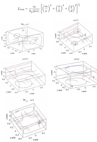
fmnp= c0 2õrr
m a
2 +
n b
2 +
p d
212
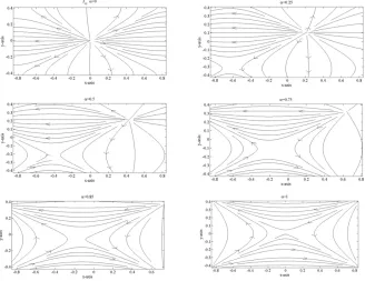
where c0 is the velocity of light. The indices m, n, p in resonance frequency relation refer to the number of variations in the standing-wave pattern in the x, y and z axes, respectively. When α = 0, the simulated result yield the original field pattern of TM mode in PEC walls cavity as shown in Fig. 1. The plot reports that the field forming loops in xz-plane is tangential magnetic field (red coloured), whereas the electric field (blue coloured) lies in xy-plane, is normal to the adjoining planes. For α = 1, the whole situation changes, in such a way that the TM mode in PEC walls cavity, transform to TE mode in PMC walls cavity. Besides this, the field pattern rotates in counter-clockwise direction by απ/2. So that the normal electric field (blue coloured) transform to tangential electric field in form of loops in xz-plane and the tangential magnetic field (red coloured) to normal magnetic field, which is the property of PMC material. For 0 < α <1, we get intermediate effects between the above mentioned results.
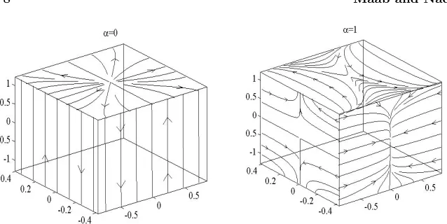
Figure 3. 3-D fractional surface current density wave patterns for two different values ofα. i.e.,α= 0 andα= 1, represent electric and magnetic surface current densities.
4. FRACTIONAL SURFACE CURRENT DENSITY
Surface current density on walls of the fractional cavity resonator is obtained using fractional TM111 fields inside the cavity resonator. Following relation has been used to obtained the fractional surface current densityJsfd
Jsfd=ˆn×Hfd
where nˆ is the outward normal to the walls of cavity and Hfd is the
fractional magnetic field intensity on the walls. In components form, we can write
Jsf d(x= 0) = −yHˆ zf d+ ˆzHyf d=−Jsf d(x=a) (12a) Jsf d(y= 0) = ˆxHzf d−zHˆ zf d =−Jsf d(y=b) (12b) Jsf d(z= 0) = −xHˆ yf d+ ˆyHxf d=−Jsf d(z=d) (12c)
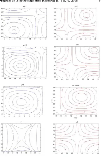
Figure 5. 2-D fractional surface current density wave patterns in xz-plane for various values of fractional orderα.
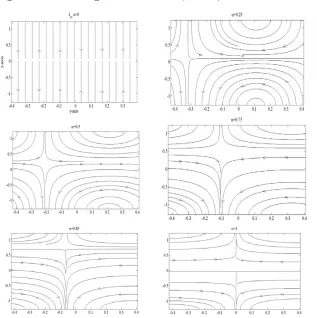
Figure 6. 2-D fractional surface current density inxy-plane for various values of fractional orderα.
5. CONCLUSIONS
In this paper we have discussed the field behavior as well as behavior of surface current density in fractional rectangular cavity resonator. When α= 0, we get the original TM field and electric surface current density in PEC walls Cavity resonator. For α = 1 the TM field and electric surface current density behavior in PEC walls cavity resonator change to TE field and magnetic surface current density in PMC walls cavity, respectively. For 0< α <1, we get intermediate steps between the two canonical cases.
REFERENCES
1. Oldham, K. B. and J. Spanier,The Fractional Calculus, Academic Press, New York, 1974.
2. Engheta, N., “Fractional curl operator in electromagnetics,”
Microw. and Opt. Techn. Lett., Vol. 17, No. 2, 86–91, 1998. 3. Naqvi, Q. A. and A. A. Rizvi, “Fractional dual solutions and
corresponding sources,” Progress In Electromagnetics Research, PIER 25, 223–238, 2000
4. Naqvi, Q. A., G. Murtaza, and A. A. Rizvi, “Fractional dual solutions to Maxwell equations in homogeneous chiral medium,”
Optics Communications, Vol. 178, 27–30, 2000.
5. Naqvi, Q. A. and M. Abbas, “Fractional duality and metamateri-als with negative permittivity and permeability,”Optics Commu-nications, Vol. 227, No. 1–3, 143–146, 2003.
6. Naqvi, Q. A. and M. Abbas, “Complex and higher order fractional curl operator in electromagnetics,” Optics Communications, Vol. 241, No. 4–6, 349–355, 2004.
7. Naqvi, S. A., Q. A. Naqvi, and A. Hussain, “Modelling of transmission through a chiral slab using fractional curl operator,”
Optics Communications, Vol. 266, No. 2, 404–406, 2006.
8. Hussain, A. and Q. A. Naqvi, “Fractional curl operator in chiral medium and fractional nonsymmetric transmission line,”Progress In Electromagnetics Research, PIER 59, 119–213, 2006.
9. Hussain, A., S. Ishfaq, and Q. A. Naqvi, “Fractional curl operator and fractional waveguides,”Progress In Electromagnetics Research, PIER 63, 319–335, 2006
10. Hussain, A., Q. A. Naqvi, and M. Abbas, “Fractional duality and perfect electromagnetic conductor (PEMC),” Progress In Electromagnetics Research, PIER 71, 85–94, 2007.
(PEMC) and fractional waveguide,”Progress In Electromagnetics Research, PIER 73, 61–69, 2007.
12. Hussain, A., M. Faryad, and Q. A. Naqvi, “Fractional curl operator and fractional chiro-waveguide,” J. ofElectromagn. Waves and Appl., Vol. 21, No. 8, 1119–1129, 2007.
13. Faryad, M. and Q. A. Naqvi, “Fractional rectangular waveguide,”
Progress In Electromagnetics Research, PIER 75, 383–396, 2007. 14. Maab, H. and Q. A. Naqvi, “Fractional surface waveguide,”
Progress In Electromagnetics Research C, Vol. 1, 199–209, 2008. 15. Veliev, E. I. and N. Engheta, “Fractional curl operator in
reflection problems,” 10th Int. Conf. on Mathematical Methods in Electromagnetic Theory, 1417, Ukraine, Sept. 2004.
16. Ivakhnychenko, M. V. and E. I. Veliev, “Fractional curl operator in radiation problems,”Mathematical Methods in Electromagnetic Theory, MMET, Conference Proceedings, 231–233, 2004.
17. Ivakhnychenko, M. V. and E. I. Veliev, “Elementary fractional dipoles,” Mathematical Methods in Electromagnetic Theory, MMET, Conference Proceedings, Art. No. 1689830, 485–487, 2006. 18. Ahmedov, T. M., M. V. Ivakhnychenko, and E. I. Veliev, “New generalized electromagnetic boundaries: Fractional operators approach,” Mathematical Methods in Electromagnetic Theory, MMET, Conference Proceedings, Art. No. 1689814, 434–436, 2006. 19. Ivakhnychenko, M. V., E. I. Veliev, and T. M. Ahmedov, “Fractional operators approach in electromagnetic wave reflection problems,” J. ofElectromagn. Waves and Appl., Vol. 21, No. 13, 1787–1802, 2007.
20. Ivakhnychenko, M. V., “Method of fractional operators in the problem of excitation of electric current thread above the plane boundary,” Telecommunications and Radio Engineering, English Translation ofElektrosvyaz and Radiotekhnika, Vol. 67, No. 2, 97– 108, 2008.
21. Ivakhnychenko, M. V., “Polarization properties of fractional fields,” Telecommunications and Radio Engineering, English Translation of Elektrosvyaz and Radiotekhnika, Vol. 67, No. 7, 567–581, 2008.
22. Lakhtakia, A., “A representation theorem involving fractional derivatives for linear homogeneous chiral media,” Microwave and Optical Technology Letters, Vol. 28, No. 6, 385–386, 2001.
23. Pozar, D. M.,Microwave Engineering, Addison-Welsey, 1990. 24. Collin, R. E., Foundations for Microwave Engineering, IEEE