Simulation without the Artificial Abort: Simplified Proof and Improved Concrete Security for Waters' IBE Scheme

A preliminary version of this paper appears inAdvances in Cryptology – EUROCRYPT ’09, Lecture Notes in Computer Science Vol. —, A. Joux ed., Springer-Verlag, 2009. This is the full version.

Simulation without the Artificial Abort:

Simplified Proof and Improved Concrete Security for

Waters’ IBE Scheme

Mihir Bellare∗ Thomas Ristenpart†

February 2009

Abstract

Waters’ variant of the Boneh-Boyen IBE scheme is attractive because of its efficency, appli-cations, and security attributes, but suffers from a relatively complex proof with poor concrete security. This is due in part to the proof’s “artificial abort” step, which has then been inherited by numerous derivative works. It has often been asked whether this step is necessary. We show that it is not, providing a new proof that eliminates this step. The new proof is not only simpler than the original one but offers better concrete security for important ranges of the parameters. As a result, one can securely use smaller groups, resulting in significant efficiency improvements.

∗_{Dept. of Computer Science & Engineering 0404, University of California San Diego, 9500 Gilman Drive, La Jolla,} CA 92093-0404, USA. Email: [email protected]. URL:http://www-cse.ucsd.edu/users/mihir. This work was supported in part by NSF grants CNS 0524765 and CNS 0627779 and a gift from Intel corporation.

Contents

1 Introduction 3

2 Definitions and Background 6

3 New Proof of Waters’ IBE without Artificial Aborts 9

4 Measuring Concrete Security 16

A Derivatives of Waters’ IBE 20

B Proof of Lemma 2.1 21

C Proof of Lemma 3.2 21

D Proof of Lemma 3.5 22

E Instantiating Pairing Parameters 23

F The BB1 Scheme and its Security 25

1

Introduction

The importance of identity-based encryption (IBE) as a cryptographic primitive stems from its widespread deployment and the numerous applications enabled by it. Since the initial work on providing realizations of IBE [8, 17], improving the efficiency, security, and extensibility of the fun-damental primitive has consequently received substantial attention from the research community. A challenging problem has been to arrive at a practical IBE scheme with a tight security reduction under standard assumptions. (The most attractive target being DBDH without relying on random oracles.) While a typical approach for progressing towards this goal is proposing new constructions, in this paper we take another route: improving the concrete security of existing constructions. This requires providing better proofs of security and analyzing the impact of their tighter reductions. Why concrete security? Informally speaking, consider an IBE scheme with a security reduction showing that attacking the scheme in time t with success probability ǫ implies breaking some believed-to-be hard problem in time t+ω1 with success probability ǫ′ ≥ ǫ/ω2. Tightness of the

reduction refers to the value of ω1 (the overhead in time needed to solve the hard problem using

the scheme attacker) and of ω2 (the amount by which the success probability decreases). Unlike

asymptotic treatments, provably-secure IBE has a history of utilizing concrete security, meaning specifyingω1 andω2 explicitly. Concrete-security for IBE started with Boneh and Franklin [8] and

has been continued in subsequent works, e.g. [6, 7, 9, 36, 21, 25] to name just a few.

As Gentry points out [21], concrete security and tight reductions are not just theoretical issues for IBE, rather they are of utmost practical import: the speed of implementations increases as ω1

and/or ω2 decrease. This is because security guarantees are lost unless the size of groups used

to implement a scheme grow to account for the magnitude of these values. In turn group size dictates performance: exponentiations in a group whose elements can be represented in r bits takes roughly_O(r3) time. As a concrete example, this means that performing four 160-bit group exponentiations can be significantly faster than asingle 256-bit group exponentiation. In practice even a factor of two efficiency slow-down is considered significant (let alone a factor of four), so finding as-tight-as-possible reductions is crucial.

Overview of IBE approaches. All practical IBE systems currently known are based on bilinear pairings. We can partition the space of such systems along two dimensions, as shown in the left table of Figure 1. In one dimension is whether one utilizes random oracles or not. In the other is the flavor of hard problem used, whether it be the basic bilinear Diffie-Hellman (BDH) assumption [8] or a q-dependent assumption such as q-BDHI [6]. Of note is that Katz and Wang [25], in the “random oracle/BDH” setting, and Gentry [21], in the “no random oracle/q-dependent setting”, have essentially solved the problem of finding practical schemes with tight reductions. On the other hand, finding practical schemes with tight reductions in the “no random oracle/BDH” setting represents a hard open problem mentioned in numerous works [6, 7, 36, 21]. This last setting turns out to be attractive for two reasons. First, from a security perspective, it is the most conservative (and consequently most challenging) with regard to choice of assumptions. Second, schemes thus far proposed in this setting follow a framework due to Boneh and Boyen [6] (so-called “commutative blinding”) that naturally supports many valuable extensions: hierarchical IBE [24], attribute-based IBE [34], direct CCA-secure encryption [10, 26], etc.

Progress in this setting is summarized in the right table of Figure 1. Boneh and Boyen initiated work here with theBB1 scheme (the first scheme in [6]). They prove it secure under the decisional

q-dependent BDH

RO model SK BF,KW

Standard model BB2,Ge BB1,Wa

Scheme Security Reduction

BB1 selective-ID polynomial

BB1 full exponential

Wa full polynomial

Figure 1: A comparison of practical IBE schemes. BF is the Boneh-Franklin scheme [8]; SK is the Sakai-Kasahara scheme [35, 16];KWis the Katz-Wang scheme [25]; BB1 and BB2 are the first and

second Boneh-Boyen schemes from [6];Wa is Waters’ scheme [36]; andGe is Gentry’s scheme [21].

(Left) The assumptions (an q-dependent assumption versus bilinear Diffie-Hellman) and model (random oracles or not) used to prove security of the schemes. (Right) Types of security offered by standard model BDH-based systems and asymptotic reduction tightness.

requires guessing the hash of the to-be-attacked identity).

Waters’ proposed a variant of BB1 that we’ll call Wa [36]. This variant requires larger public

parameters, but can be proven fully secure with a polynomial reduction to DBDH that does not use random oracles. The relatively complex security proof relies on a novel “artificial abort” step, that, while clever, is unintuitive. It also significantly hurts the concrete security and, thereby, efficiency of the scheme. Many researchers in the community have asked whether artificial aborts can be dispensed with, but the general consensus seems to have been that the answer is “no” and that the technique is somehow fundamental to proving security. This folklore assessment (if true) is doubly unfortunate because Wa, inheriting the flexibility of the Boneh-Boyen framework, has been used in numerous diverse applications [10, 1, 5, 30, 13, 14, 22, 26]. As observed in [26], some of these subsequent works offer difficult to understand (let alone verify) proofs, due in large part to their use of the artificial abort technique in a more-or-less black-box manner. They also inherit its concrete security overhead.

This paper. Our first contribution is to provide a novel proof of Waters’ variant that completely eliminates the artificial abort step. The proof, which uses several new techniques and makes crucial use of code-based games [4], provides an alternate and (we feel) more intuitive and rigorous approach to proving the security of Wa. Considering the importance of the original proof (due to its direct or indirect use in [10, 1, 5, 30, 13, 14, 22, 26]), a more readily understood proof is already a significant contribution. Our reduction (like Waters’) is not tight, but as we see below it offers better concrete security for many important parameter choices, moving us closer to the goal of standard model BDH-based schemes with tight reductions. The many Waters’-derived works [10, 1, 5, 30, 13, 14, 22, 26] inherit the improvements in concrete security. We briefly describe these derivatives in Appendix A.

We now have the BB1 and Wa schemes, the former with an exponentially-loose reduction and

κ ǫ q sBB sW sBR TEnc(sW)/TEnc(sBR)

60 2−20

220

192 192 128 9

70 2−20

220 256 192 128 9

80 2−30

230

256 256 192 5

90 2−30

230

– 256 192 5

100 2−10 210 – 128 192 1/9

100 2−40

240

– 256 192 5

192 2−40

240 – 256 – –

Figure 2: Table showing the security level of the pairing setups required to achieveκ-bits of security for the BB1 andWaencryption schemes when adversaries achieveǫsuccess probability usingq key

extraction queries. Loosely speaking, the security level of the pairing setup is (logp)/2 wherep is the size of the first pairing group. HeresBB,sW,sBR are, respectively, the securities of the pairing

setups for BB1,Wa under Waters’ reduction, and Wa under the new reduction. The final column

represents the (approximate) ratio of encryption times forWa as specified by the two reductions. A dash signifies that one needs a pairing setup of security greater than 256.

challenging.

Let us first mention the high-level results, before explaining more. In the end our framework implies that Waters’ variant usually provides faster standard model encryption (than BB1). Our

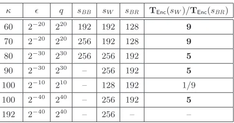
new proof provides a better reduction for low to mid range security parameters, while Waters’ reduction is tighter for higher security parameters. The new reduction in fact drastically improves efficiency in the former category, offering up to 9 times faster encryption for low parameters and 5 times faster encryption for mid-range security levels. Where Waters’ reduction is tighter, we can continue to choose group size via it; the new reduction never hurts efficiency.

BB1 does better than Wa when identities are short, such as n = 80 bits. We have,

how-ever, focused on providing IBE with arbitrary identity spaces, which provides the most versatility. Supporting long identities (e.g. email addresses such as [email protected]) requires utilizing a collision-resistant hash function to compress identities. In this case, the birthday bound mandates that the bit lengthnof hash outputs be double the desired security level, and this affects theBB1 scheme more due to its reduction being loose by a factor of 2n.

Framework details. We present some results of applying our framework in Figure 2. Let us explain briefly what the numbers signify and how we derived them. (Details are in Section 4.) By a setup we mean groups G_1,G_2,G_{T admitting a bilinear map e:} G_{1 ×}G_{2 →} G_{T. The setup} provides securitys(bits) if the best known algorithms to solve the discrete logarithm (DL) problem take at least 2s _{time in any of the three groups. We assume (for these estimates but not for the}

proof!) that the best algorithm for solving DBDH is solving DL in one of the groups. An important practical issue in pairings-based cryptography is that setups for arbitrary security are not known. Accordingly, we will restrict attention to valuess= 80, 112, 128, 192, and 256, based on information from [31, 27, 28, 18, 19]. Figure 6 in Appendix E shows representation sizes of the corresponding groups. Now we take as our target that the IBE scheme should provideκ bits of security. By this we mean that any adversary making at most q = 1/ǫ Extract queries and having running time at mostǫ2κ _{should have advantage at mostǫ. For each scheme/reduction pair we can then derive}

Other related work and open problems. Recently Hofheinz and Kiltz describe programmable hash functions [23]. Their main construction uses the same hash function (originally due to Chaum et al. [15]) as Waters’, and they provide new proof techniques that provide a√n(nis the length of identities) improvement on certain bounds that could be applicable to Wa. But this will only offer a small concrete security improvement compared to ours. Moreover, their results are asymptotic and hide (seemingly very large) unknown constants.

As mentioned, providing a scheme based on DBDH that has a tight security reduction (without random oracles) is a hard open problem, and one that remains after our work. (One reason we explain this is that we have heard it said that eliminating the artificial abort would solve the open problem just mentioned, but in fact the two seem to be unrelated.) Finding a tight reduction for Waters’ (or another BB1-style scheme) is of particular interest since it would immediately give

a hierarchical IBE (HIBE) scheme with security beyond a constant number of levels (the best currently achievable). From a practical point of view we contribute here, since better concrete security improves the (constant) number of levels achievable. From a theoretical perspective, this remains an open problem.

Viewing proofs as qualitative. We measure efficiency of schemes when one sets group size according to the best-known reduction. However, the fact that a proof implies the need for groups of certain size to guarantee security of the scheme does not mean the scheme is necessarily insecure (meaning there is an attack) over smaller groups. It simply means that the proof tells us nothing about security in these smaller groups. In the context of standards it is sometimes suggested one view a proof as a qualitative rather than quantitative guarantee, picking group sizes just to resist the best known attack. Our sense is that this procedure is not viewed as ideal even by its proposers but rather forced on them by the looseness of reductions. To rectify this gap, one must find tighter reductions, and our work is a step to this end.

2

Definitions and Background

Notation. We fix pairing parameters GP = (G_1,G_2,G_{T, p,e, ψ) where}G_1,G_2, G_{T are groups of} prime order p; e: G_{1 ×}G_{2 →} G_{T is a non-degenerate, efficiently computable bilinear map; and} ψ: G_2→G_{1 is an efficiently computable isomorphism [8]. LetTexp(}G_{) denote the time to compute} an exponentiation in a groupG_{. Similarly, letTop(}G_{) denote the time to compute a group operation} in a groupG_{. LetTψ denote the time to computeψ. Let}G∗ ₌G_{−{1}denote the set of generators} of G_{where1 is the identity element of}G_.

Vectors are written in boldface, e.g. u _∈ Zn+1

p is a vector of n+ 1 values each in Zp. We

denote theith

component of a vector u by u[i]. If S _{∈ {}0,1_}∗ then _|S_| denotes its length andS[i] denotes its ith

bit. For integers i, j we let [i .. j] = _{i, . . . , j_}. The running time of an adversary

A is denotedT(_A). We use big-oh notation with the understanding that this hides a small, fixed, machine-dependent constant.

procedure Initialize: g2

$

←G∗

2;g1 ←ψ(g2) ;a, b, s $

←Z_{p;d← {}$ _0,1} Ifd= 1 thenW _←$ e(g1, g2)abs Else W

$

←G_T Ret (g1, g2, g2a, g2b, gs2, W)

Game DBDHGP

procedure Finalize(d′_):

Ret (d′_=d) procedure Initialize:

(mpk, msk)_←$ Pg;c_{← {}$ 0,1_} Retmpk

procedure Extract(I): RetKg(mpk, msk, I)

Game IND-CPAIBE procedure LR(I, M0, M1):

RetEnc(mpk, I, Mc) procedure Finalize(c′): Ret (c′ _=c)

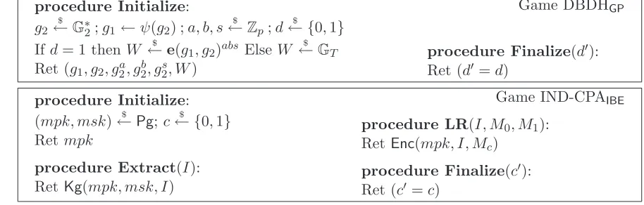
Figure 3: The DBDH and IND-CPA games.

if their code differs only in statements that follow the setting of badto true. (For examples, games G0, G1 of Figure 4 are identical-until-bad, as they differ only in the boxed statements.) We let

“GA_i setsbad” denote the event that game Gi, when executed with adversary A, sets badto true

(and similarly for “GA_i doesn’t setbad”). It is shown in [4] that if Gi,Gj are identical-until-badand A is an adversary, then

PrGA_i setsbad= PrGA_j setsbad. (1) The fundamental lemma of game-playing [4] says that if Gi,Gj are identical-until-badthen for anyy

PrGA_{i ⇒}y₋PrG_jA _⇒y_≤PrGA_i setsbad.

This lemma is useful when the probability thatbadis set is small, but in our setting this probability will be close to one. We will instead use the following variant:

Lemma 2.1 Let Gi,Gj be identical-until-badgames and let A be an adversary. Then for anyy

PrGA_{i ⇒}y_∧GA_i doesn’t setbad= PrGA_{j ⇒}y_∧GA_j doesn’t setbad.

Lemma 2.1 is implicit in the proof of the fundamental lemma of [4], but for completeness we provide a proof in Appendix B. Lemma 2.1 was also used in [3, 33].

DBDH problem. The Decisional Bilinear Diffie-Hellman (DBDH) assumption (in the asymmetric setting) [6] is captured by the game described in Figure 3. We define the dbdh-advantage of an adversary_A againstGP= (G_1,G_2,G_{T, p,e, ψ) by}

Advdbdh_GP (_A) = 2_·PrDBDHA_GP⇒true₋1. (2) Identity-based encryption. Anidentity-based encryption (IBE) schemeis a tuple of algorithms

(ind-cpa). The ind-cpa advantage of an adversary_A against an IBE schemeIBEis defined by

Advind-cpa_IBE (_A) = 2_·PrIND-CPAA_IBE⇒true₋1, (3) where game IND-CPA is shown in Figure 3. We only allow legitimate adversaries, where adver-sary _A is legitimate if it makes only one query (I∗, M0, M1) to LR, for some I∗ ∈ IdSp and

M0, M1 ∈MsgSp with|M0|=|M1|, and never queries I∗ toExtract. Here|M|denotes the length

of some canonical string encoding of a messageM _∈MsgSp. (In the schemes we consider messages are group elements.)

Note that we do allow multiple queries to Extract with the same identity, which is important because key generation in the schemes we consider are randomized. When we say that _A makes at mostq oracle queries or has running time at most twe mean that this is true regardless of _A’s coins and environment, meaning even if its input and the answers to its oracle queries do not come from IND-CPAIBE.

Waters’ IBE scheme. The Boneh-Boyen IBE scheme is described in Appendix F. The Wa-ters’ IBE scheme changes the hash function used byBB1. Let n be a positive integer. Define the

hash family H: Gn+1

1 × {0,1}n → G1 by H(u, I) = u[0]Qni=1u[i]I[i] for any u ∈ Gn1+1 and any

I _{∈ {}0,1_}n_{. The Waters IBE schemeWa= (Pg,Kg,Enc,Dec) associated toGPandnhas associated}

identity spaceIdSp=_{0,1_}n _{and message spaceMsgSp=G}

T, and its first three algorithms are as

follows:

procedure Pg

A1 $

←G_{1;g2 ←}$ G∗

2

b_←$ Z_{p;B2 ←g}b

2;u $

←Gn+1

1

mpk_←(g2, A1, B2,u)

msk_←Ab

1

Ret (mpk, msk)

procedure Kg(mpk, msk, I) (g2, A1, B2,u)←mpk

K _←msk;r_←$ Z_p Ret (K_·H(u, I)r_{, g}r

2)

procedure Enc(mpk, I, M) (g2, A1, B2,u)←mpk

s_←$ Z_p

Ret (e(A1, B2)s·M, gs2, H(u, I)s)

Above, when we write (g2, A1, B2,u) ← mpk we mean mpk is parsed into its constituent parts.

We do not specify the decryption algorithm since it is not relevant to IND-CPA security; it can be found in [36].

In [36] the scheme is presented in the symmetric setting where G_{1 =} G_{2. While this makes} notation simpler, we work in the asymmetric setting because it allows pairing parameters for higher security levels [19].

The hash functions used by Boneh-Boyen and Waters’ schemes have restricted domain. One can extend to IdSp=_{0,1_}∗ by first hashing an identity with a collision-resistant hash function to derive ann-bit string. (ForBB1 this is then encoded in some canonical fashion to a point inZp.)To

ensure security from birthday attacks, the output lengthnof the CR function must have bit-length at least twice that of the desired security parameter.

Waters’ result. Waters [36] proves the security of theWascheme associated toGP, nunder the assumption that the DBDH problem in GP is hard. Specifically, let _A be an ind-cpa adversary againstWathat runs in time at most t, makes at most q_∈[1.. p/4n] queries to itsExtractoracle and has advantageǫ=Advind-cpa_Wa (_A). Then [36, Theorem 1] presents a dbdh-adversary_BWa such that

Advdbdh_GP (_BWa) _≥ ǫ

32(n+ 1)q , and (4)

where

Tsim(n, q) = O(Tψ+ (n+q)·Texp(G1) +q·Texp(G2) +qn+Top(GT)) (6) Tabort(ǫ, n, q) = O(q2n2ǫ−2ln(ǫ−1) ln(qn)). (7)

An important factor in the “looseness” of the reduction is the Tabort(ǫ, n, q) term, which can be

very large, making T(_BWa) much more than T(_A). This term arises from the “artificial abort” step. (In [36], the Tabort(ǫ, n, q) term only has a qn factor in place of the q2n2 factor we show.

However, the step requires performing q times up to noperations over the integers modulo 4q for each of the ℓ=_O(qnǫ−2_lnǫ−1_{lnqn) vectors selected, so our term represents the actual cost.)}

3

New Proof of Waters’ IBE without Artificial Aborts

We start with some high-level discussion regarding Waters’ original proof and the reason for the artificial abort. First, one would hope to specify a simulator that, given IND-CPA adversary _A that attacks the IBE scheme using q Extract queries and gains advantage ǫ, solves the DBDH problem with advantage not drastically worse thanǫ. But_Acan makeExtract queries that force any conceivable simulator to fail, i.e. have to abort. This means that the advantage against DBDH is conditioned on_A not causing an abort, and so it could be the case that_A achievesǫadvantage in the normal IND-CPA experiment but almost always causes aborts for the simulator. In this (hypothetical) case, the simulator could not effectively make use of the adversary, and the proof fails.

On the other hand, if one can argue that the lower and upper bounds on the probability of _A causing an abort to occur are close (i.e. the case above does not occur), then the proof would go through. As Waters’ points out [36], the natural simulator (that only aborts when absolutely nec-essarily) fails to provide such a guarantee. To compensate, Waters’ introduced “artificial aborts”. At the end of a successful simulation for the IBE adversary, the simulator _BWa used by Waters’

generates _O(qnǫ−2_lnǫ−1_{lnqn) random vectors. These are used to estimate the probability that}

theExtract queries made by _A cause an abort during any given execution of the simulator. The simulator then artificially aborts with some related probability. Intuitively, this forces the proba-bility of aborting to be independent of_A’s particular queries. Waters’ shows that_BWaprovides the

aforementioned guarantee of close lower and upper bounds and the proof goes through.

The artificial abort step seems strange because_BWais forcing itself to fail even when it appears

to have succeeded. The concrete security also suffers because the running time of the simulator goes up byTabort(ǫ, n, q) as shown in (7).

The rest of this section is devoted to proving the next theorem, which establishes the security of the Waters’ IBE scheme without relying on an artificial abort step.

Theorem 3.1 Fix pairing parameters GP = (G_1,G_2,G_{T, p,e, ψ) and an integer n ≥ 1, and let}

Wa= (Pg,Kg,Enc,Dec) be the Waters IBE scheme associated to GP and n. Let _A be an ind-cpa adversary againstWawhich has advantageǫ=Advind-cpa_Wa (_A)>0 and makes at mostq _∈[1.. pǫ/9n] queries to itsExtract oracle. Then there is a dbdh adversary _Bsuch that

Advdbdh_GP (_B) _≥ ǫ

2

27qn+ 3ǫ , and (8)

T(_B) = T(_A) +Tsim(n, q) (9)

The limitations on q—namely, 1 _≤q _≤p/4n in Waters’ result and 1_≤q _≤pǫ/9n in ours—are of little significance since in practice p_≥2160_{, ǫ≥2}−80_{, andn= 160. For q = 0 there is a separate,}

tight reduction. The remainder of this section is devoted to the proof of Theorem 3.1.

Some definitions. Letm =_⌈9q/ǫ_⌉and let X = [₋n(m₋1)..0]_×[0.. m₋1]_{× · · · ×}[0.. m₋1] where the number of copies of [0.. m₋1] is n. Forx_∈X,y_∈Z_pn+1 _{and I ∈ {0,1}}n _{we let}

F(x, I) =x[0] +

n X

i=1

x[i]I[i] and G(y, I) =y[0] +

n X

i=1

y[i]I[i] modp . (10) Note that while the computation ofGabove is over Z_{p, that ofF is over} Z_.

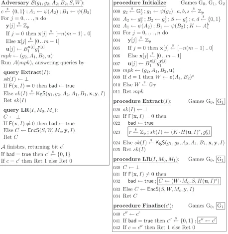
Adversary _B. Our DBDH adversary_Bis depicted in Figure 4, where the simulation subroutines

KgSandEncSare specified below. There are two main differences between our adversary and that of Waters’. The first is that in our case the parametermis_O(q/ǫ) while in Waters’ case it is_O(q). The second difference of course is that Waters’ adversary _BWa, unlike ours, includes the artificial

abort step. Once _A has terminated, this step selects l = _O(qnǫ−2_ln(ǫ−1_{) ln(qn)) new random}

vectors x1, . . . ,xl from X. Letting I1, . . . , Iq denote the identities queried by A to its Extract

oracle and I0 the identity queried to the LR oracle, it then evaluates F(xi, Ij) for all 1 ≤ i ≤ l

and 0 _≤ j _≤ q, and uses these values to approximate the probability that bad is set. It then aborts with some related probability. Each computation ofFtakes_O(n) time, and there areq such computations for each of the l samples, accounting for the estimate of (7). In addition there are some minor differences between the adversaries. For example, xis chosen differently. (In [36] it is taken from [0.. m₋1]n+1_{, and an additional valuek∈[0.. n], which we do not have, is mixed in.)}

We note that our adversary in fact never aborts. Sometimes, it is clearly returning incorrect answers (namely_⊥) to_A’s queries. Adversary_Awill recognize this, and all bets are off as to what it will do. Nonetheless, _B continues the execution of _A. Our analysis will show that _B has the claimed properties regardless.

An analysis of the running time of _B, justifying equations (6) and (9), is given in Appendix G. Simulation subroutines. We define the subroutines that _Butilizes to answer Extractand LR

queries. We say that (g1, g2, A2, A1, B2, B1,x,y,u, S, W) are simulation parameters if: g2 ∈ G∗2;

g1 = ψ(g2) ∈ G∗1; A2 ∈ G2; A1 = ψ(A2) ∈ G1; B2 ∈ G2; B1 = ψ(B2) ∈ G1; x ∈ X; y ∈ Znp+1; u[j] =B₁x[j]g₁y[j] forj_∈[0.. n];S _∈G_{2; and W ∈}G_{T. We define the following procedures:}

procedure KgS(g1, g2, A2, A1, B1,x,y, I)

r_←$ Z_{p;w←F(x, I)}−1 _modp L1←B1F(x,I)·rg

G(y,I)·r

1 A

−G(y,I)w

1

L2←g2rA−w2

Ret (L1, L2)

procedure EncS(S, W, M,y, I) C1 ←W ·M

C2 ←S;C3 ←ψ(S)G(y,I)

Ret (C1, C2, C3)

Note that ifF(x, I)₆= 0 thenF(x, I)_6≡0 (modp) so the quantitywcomputed byKgSis well-defined whenever F(x, I)₆= 0. This is because the absolute value of F(x, I) is at most

n(m₋1) =n

9q ǫ

−1

< 9nq

ǫ ≤p , (11)

the last because of the restriction on q in the theorem statement. The next lemma captures two facts about the simulation subroutines, which we will use in our analysis.

Lemma 3.2 Let (g1, g2, A2, A1, B2, B1,x,y,u, S, W) be simulation parameters. Let I ∈ {0,1}n.

Adversary _B(g1, g2, A2, B2, S, W):

c_{← {}$ 0,1_};A1 ←ψ(A2) ;B1 ←ψ(B2)

For j= 0, . . . , n do

y[j]_←$ Z_p

If j= 0 thenx[j]_←$ [₋n(m₋1)..0] Else x[j]_←$ [0.. m₋1]

u[j]_←B₁x[j]g₁y[j] mpk _←(g2, A1, B2,u)

Run _A(mpk), answering queries by

query Extract(I): sk(I)_{← ⊥}

IfF(x, I) = 0 thenbad_←true

Else sk(I)_←$ KgS(g1, g2, A2, A1, B1,x,y, I)

Retsk(I)

query LR(I, M0, M1):

C_{← ⊥}

IfF(x, I)₆= 0 then bad_←true

Else C_←EncS(S, W, Mc,y, I)

RetC

A finishes, returning bitc′

If bad=true thenc′ $

← {0,1_} If c=c′ then Ret 1 else Ret 0

procedure Initialize: Games G0, G1, G2

000 g2 $

←G∗

2;g1 ←ψ(g2) ;a, b, s $

←Z_p 001 A2 ←g2a;B2←gb2;S←g2s;c, d

$

← {0,1_} 002 A1 ←ψ(A2) ;B1 ←ψ(B2) ;K←Ab1

003 Forj= 0, . . . , ndo 004 y[j]_←$ Z_p

005 Ifj= 0 thenx[j]_←$ [₋n(m₋1)..0] 006 Elsex[j]_←$ [0.. m₋1]

007 u[j]←Bx₁[j]gy₁[j] 008 mpk_←(g2, A1, B2,u)

009 Ifd= 1 thenW _←e(A1, B2)s

010 ElseW _←$ G_T 011 Retmpk

procedure Extract(I): Games G0, G1

020 sk(I)_{← ⊥}

021 IfF(x, I) = 0 then 022 bad_←true

023 r←$ Z_{p;sk(I)←(K·H(u, I)}r_{, g}r

2)

024 Elsesk(I)←$ KgS(g1, g2, A2, A1, B1,x,y, I)

025 Retsk(I)

procedure LR(I, M0, M1): Games G0, G1

030 C_{← ⊥}

031 IfF(x, I)₆= 0 then

032 bad_←true; C _←(W_·Mc, S, H(u, I)s)

033 ElseC ←EncS(S, W, Mc,y, I)

034 RetC

procedure Finalize(c′_{): Games G}

0, G1

040 c′′_←c′

041 Ifbad=truethenc′′ $

← {0,1_}; c′′_←c′

042 Ifc=c′′ then Ret 1 else Ret 0

Figure 4: Adversary_Band the start of the game sequence. Game G1 includes the boxed statements

in procedures Extract,LR, and Finalize while G0 does not.

the discrete log of S to base g2. Then ifF(x, I) 6= 0 the outputs of KgS(g1, g2, A2, A1, B1,x,y, I)

and Kg(mpk, msk, I) are identically distributed. Also ifF(x, I) = 0 then for any M _∈MsgSp, the output ofEncS(S, W, M,y, I) is (W_·M, S, H(u, I)s_).

The proof of Lemma 3.2, which follows arguments given in [36], is given in Appendix C.

Overview. Consider executing _B in game DBDHGP. If d = 1, then Lemma 3.2 implies that

procedure Extract(I): Game G2

220 If F(x, I) = 0 thenbad_←true

221 r _←$ Z_{p; Ret sk(I)←(K·H(u, I)}r_{, g}r

2)

procedure LR(I, M0, M1): Game G2

230 If F(x, I)₆= 0 thenbad_←true

231 Ret C_←(W_·Mc, S, H(u, I)s)

procedure Finalize(c′_{): Game G}

2

240 If c=c′ then Ret 1 else Ret 0

procedure Initialize: Game G3

300 A1 $

←G_1;g2←$ G∗

2;b, s $

←Z_p;cnt←0 301 B2 ←g2b;S ←g2s;c, d

$

← {0,1_};K_←Ab

1

302 For j= 0, . . . , ndo 303 z[j]_←$ Z_p;u[j]←gz[j]

1

304 If j= 0 thenx[j]_←$ [₋n(m₋1)..0] 305 Else x[j]_←$ [0.. m₋1]

306 y[j]_←z[j]₋b_·x[j] modp 307 mpk _←(g2, A1, B2,u)

308 If d= 1 thenW _←e(A1, B2)s

309 Else W _←$ G_T 310 Ret mpk

procedure Finalize(c′): Game G3

340 For j= 1, . . . , cntdo

341 If F(x, Ij) = 0 then bad←true

342 If F(x, I0)6= 0 thenbad←true

343 If c=c′ then Ret 1 else Ret 0

procedure Initialize: Game G4

400 A1 $

←G_{1;g2 ←}$ G∗

2;b, s $

←Z_p;i←0 401 B2 ←g2b;S ←gs2;c, d

$

← {0,1_};K_←Ab₁ 402 Forj= 0, . . . , ndo

403 z[j]_←$ Z_p;u[j]←gz[j] 404 mpk_←(g, A1, B2,u)

405 Ifd= 1 thenW _←e(A1, B2)s

406 Else W _←$ G_T 407 Retmpk

procedure Extract(I): Games G3, G4

320 cnt_←cnt+ 1 ;Icnt←I

321 r_←$ Z_{p; Retsk(I)←(K·H(u, I)}r_{, g}r

2)

procedure LR(I, M0, M1): Games G3, G4

330 I0←I

331 RetC_←(W_·Mc, S, H(u, I)s)

procedure Finalize(c′): Game G4

440 Forj= 0, . . . , ndo

441 Ifj= 0 thenx[j]_←$ [₋n(m₋1)..0] 442 Elsex[j]_←$ [0.. m₋1]

443 Forj= 1, . . . , cntdo

444 IfF(x, Ij) = 0 thenbad←true

445 IfF(x, I0)6= 0 thenbad←true

446 Ifc=c′ _{then Ret 1 else Ret 0}

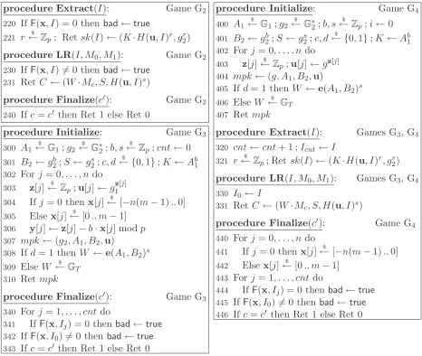
Figure 5: Continuation of the game sequence. Games G2 and G1 (see Figure 4) have identical

Initializeprocedures. Games G3 and G4 have identicalExtract and LR procedures.

could show that the setting of badis independent of the correctness of_B’s output, then one could conclude by multiplying the probabilities of these events. The difficulty in the proof is that this independence does not hold. Waters’ artificial abort step is one way to compensate. However, we have dropped this (expensive) step and propose nonetheless to push an argument through. We will first use the game sequence G0–G4 to arrive at a game where the choice ofxis independent of the

game output. The subtle point is that thisstill does not provide independence between settingbad

G0−G4 to move fromBrunning in the DBDH experiment to a game G4 (shown in Figure 5) that

is essentially the IND-CPA experiment, though with some additional bookkeeping. This transition is critical since it moves to a setting where the choice of x is clearly independent of _A’s choices. We capture this game playing sequence via the following lemma. Let GD4 denote the event that

GA

4 does not set bad.

Lemma 3.3 Advdbdh_GP (_B) = 2_·PrGA_{4 ⇒}d_∧GD4−Pr [GD4]

Proof: Figures 4 and 5 compactly describe four games showing next to each procedure the games in which it appears. For example, the Initialize procedure of Figure 4 is common to games G0,

G1, and G2. Let BDi denote the event that GiA sets bad and GDi the event that GAi does not

set bad, for 0 _≤i _≤4. The Initialize procedure of game G0 includes the code of the Initialize

procedure of game DBDHGP. Game G0 and adversaryBanswerA’s oracle queries in the same way

(remember that G0 omits the boxed statements). The output of G0 (as computed by itsFinalize

procedure) is the same as_B’s. (The code is written differently but is equivalent.) The bitdin G0

represents the challenge bit of the same name in game DBDHGP. Thus we have,

PrDBDHB_GP⇒true = PrGA_{0 ⇒}d

= PrGA_{0 ⇒}d _| BD0Pr [BD0] + PrGA0 ⇒d∧GD0.

If GA₀ sets bad then line 041 ensures that c′′ is random. Line 042 then ensures that the output of G0 is random as well and thus equals dwith probability 1/2. This means that the conditional

probability above is 1/2 and hence we have PrDBDHB_GP⇒true= 1

2·Pr [BD0] + Pr

GA_{0 ⇒}d_∧GD0. (12)

The boxed statements of lines 023 and 032 of G1 are “corrections” which ensure that no oracle

query ever returns_⊥, even in the case that a subroutine would fail, meaning whenbadis set. (Note this code uses the secret keyK and the discrete logsofS, neither of which were given to_Bor used by G0 to respond to oracle queries.) But G0,G1 are identical-until-bad, so by (1) and Lemma 2.1

we have

Pr [BD0] = Pr [BD1] and PrGA0 ⇒d∧GD0= PrGA1 ⇒d∧GD1. (13)

Let us now consider how G1 relates to G2. Lemma 3.2 tells us thatKgSat line 024 and the code of

line 023 compute the same valuesk(I). Lemma 3.2 also tells us that EncSat line 033 and the code of line 032 compute the same tuple C. (Recall_A is allowed only oneLR query.) Thus, G1 always

answers oracle queries in the same manner, meaning one can equivalently define its Extract and

LR procedures as in game G2. Since the boxed code of line 041 is included in G1, we always have

c′′ _=c′ _{and hence the output of the game is simply 1 if c = c}′ _{and 0 otherwise. This is how G}

2

computes its output at 240. It follows that

Pr [BD1] = Pr [BD2] and PrGA1 ⇒d∧GD1= PrGA2 ⇒d∧GD2. (14)

TheExtractandLRprocedures of G2may setbadbut do not use it. Throwing in the bookkeeping

of lines 300, 320, and 330, we can thus move the code setting bad into lines 340–342 in G3. We

then observe that lines 004–007 of G2 can equivalently be written as lines 303–306 of G3. Finally,

game G2 no longer uses g1,A2, and B1. Thus we re-write lines 000–002 of G2 as 300–301 of G3.

The distribution ofA1 is equivalent in both games. At this point we have

Pr [BD2] = Pr [BD3] and PrGA2 ⇒d∧GD2= PrGA3 ⇒d∧GD3. (15)

pickingx untilFinalize and dropsy, but otherwise its code matches that of G3. Thus we have

Pr [BD3] = Pr [BD4] and PrGA3 ⇒d∧GD3= PrGA4 ⇒d∧GD4. (16)

Using equations (2), (12), (13), (14), (15), and (16) we have

Advdbdh_GP (_B) = 2_·PrDBDHB_GP⇒true₋1

= Pr [BD4] + 2·PrG4A⇒d∧GD4−1

= 2_·PrGA_{4 ⇒}d_∧GD4−Pr [GD4]. (17)

This completes the proof of Lemma 3.3.

We now reach a subtle point. Consider the following argument: “The event GD4 depends only

on x, which is chosen at lines 440–442 after the adversary and game outputs are determined. So

GD4 is independent of the event that GA4 ⇒d.” If we buy this, the probability of the conjunct in

Lemma 3.3 becomes the product of the probability of the constituent events, and it is quite easy to conclude. However, the problem is that the argument in quotes above is wrong. The reason is that

GD₄ also depends on I0, . . . , Iq and these are adversary queries whose values are not independent

of the game output. Waters’ compensates for this via the artificial abort step, but we do not have this step in _Band propose to complete the analysis anyway.

Conditional independence lemma. Let

ID=_{(I0, . . . , Iq)∈({0,1}n)q+1 : ∀i∈[1.. q] (I06=Ii)}.

For (I0, . . . , Iq)∈ID let

γ(I0, . . . , Iq) = Pr [F(x, I0) = 0∧F(x, I1)6= 0∧ · · · ∧F(x, Iq)6= 0 ]

where the probability is taken over x _←$ X. This is the probability of GD4 under a particular

sequence of queried identitiesI0, . . . , Iq. (We stress that here we first fixI0, . . . , Iq and then choose x at random.) If γ(I0, . . . , Iq) were the same for all (I0, . . . , Iq) ∈ ID then the problem discussed

above would be resolved. The difficulty is thatγ(I0, . . . , Iq) varies withI0, . . . , Iq. Our next lemma

is the main tool to resolve the independence problem. Roughly it says that if we consider the conditional space obtained by conditioning on a particular sequenceI0, . . . , Iq of queried identities,

then independence does hold. To formalize this, let Q(I) be the event that the execution of G4

with_A results in the identities I0, . . . , Iq being queried byA, where I= (I0, . . . , Iq). Then: Lemma 3.4 For anyI_∈ID,

PrGA_{4 ⇒}d_∧GD_4∧Q(I) = γ(I)_·PrGA_{4 ⇒}d_∧Q(I) (18) Pr [GD4∧Q(I) ] = γ(I)·Pr [Q(I) ] (19)

Proof: The set of coin tosses underlying the execution of G4 with A can be viewed as a cross

product Ω = Ω′_×X, meaning each member ω of Ω is a pair ω = (ω′,x) where x is the choice made at lines 440–442 and ω′ _{is all the rest of the game and adversary coins. For any I ∈ID let}

Ω′_{(I) be the set of allω ∈Ω}′ _{such that the execution withω produces Ias the sequence of queried}

identities. (WhichIis produced depends only onω′ sincexis chosen after_Ahas terminated.) Let Ω′

out be the set of allω ∈Ω′ on which the execution outputsd. (Again, this is determined only by

ω′ _{and not x.) Let X}

gd(I) be the set of allx∈X such that

where I= (I0, . . . , Iq). Now observe that the set of coins leading to G₄A ⇒ dis Ω′_out×X and the

set of coins leading to GD4∧Q(I) is Ω′(I)×Xgd(I). So

PrGA_{4 ⇒}d_∧GD4∧Q(I) = |

(Ω′

out×X)∩(Ω′(I)×Xgd(I))|

|Ω′_×X|

= |(Ω

′

out∩Ω′(I))×Xgd(I)|

|Ω′_×X| =

|Ω′_out∩Ω′(I)_{| · |}Xgd(I)|

|Ω′_{| · |X|}

= |Ω

′

out∩Ω′(I)| · |X|

|Ω′_{| · |X|} ·

|Xgd(I)|

|X_| =

|(Ω′

out∩Ω′(I))×X|

|Ω′_×X| ·

|Xgd(I)|

|X_| .

But the first term above is PrGA

4 ⇒d∧Q(I)

while the second is γ(I), establishing (18). For (19) we similarly have

Pr [GD4∧Q(I) ] = |

Ω′_(I)×X

gd(I)|

|Ω′_×X| =

|Ω′(I)_|

|Ω′_| ·

|Xgd(I)|

|X_|

= |Ω

′_{(I)| · |X|} |Ω′_{| · |X|} ·

|Xgd(I)|

|X_| =

|Ω′_(I)×X| |Ω′_×X| ·

|Xgd(I)|

|X_| .

But the final terms above are Pr [Q(I) ] and γ(I), respectively, establishing (19).

Analysis continued. Letγmin be the smallest value of γ(I0, . . . , Iq) taken over all (I0, . . . , Iq)∈

ID. Letγmaxbe the largest value ofγ(I0, . . . , Iq) taken over all (I0, . . . , Iq)∈ID. Using Lemma 3.3

we have that

Advdbdh_GP (_B) = 2_·PrG₄A_⇒d_∧GD4−Pr [GD4]

= X

I∈ID

2_·PrGA_{4 ⇒}d_∧GD4∧Q(I)−

X

I∈ID

Pr [GD4∧Q(I) ]

and applying Lemma 3.4:

Advdbdh_GP (_B) = X

I∈ID

2γ(I)_·PrGA_{4 ⇒}d_∧Q(I)₋X

I∈ID

γ(I)_·Pr [Q(I) ]

≥ γmin

X

I∈ID

2_·PrGA_{4 ⇒}d_∧Q(I)

| {z }

=2·Pr[GA

4⇒d]

−γmax

X

I∈ID

Pr [Q(I) ]

| {z }

=1

≥ 2γmin·PrGA4 ⇒d

−γmax. (20)

Now

PrGA_{4 ⇒}d = PrGA_{4 ⇒}1 _| d= 1Pr [d= 1 ] + PrGA_{4 ⇒}0 _| d= 0Pr [d= 0 ]

= 1

2 ·Pr

GA_{4 ⇒}1 _| d= 1+1 2 ·Pr

GA_{4 ⇒}0 _| d= 0

= 1 2 · 1 2 + 1 2·Adv

ind-cpa

Wa (A) +1 2· 1 2 (21) = 1

4 ·Adv

ind-cpa

Wa (A) +

1

where we justify (21) as follows. In the case that d = 0, the value W is uniformly distributed overG_{T and hence line 331 gives Ano information about the bitc. So the probability that c=c}′ at line 446 is 1/2. On the other hand if d = 1 then G4 implements the IND-CPAWa game, so

2_·PrGA_{4 ⇒}1 _| d= 1₋1 =Advind-cpa_Wa (_A) by (3). We substitute (22) into (20) and get

Advdbdh_GP (_B) _≥ 2γmin

1 4Adv

ind-cpa

Wa (A) +

1 2

−γmax

= γmin 2 Adv

ind-cpa

Wa (A) + (γmin−γmax). (23)

To finish the proof, we use the following:

Lemma 3.5 1

n(m₋1) + 1

1₋ q m

≤γmin≤γmax≤

1

n(m₋1) + 1

The proof of Lemma 3.5, based on ideas in [36], is given in Appendix D. Letα = 1/(n(m₋1) + 1). Recall that m = _⌈9q/ǫ_{⌉ ≥}9q/ǫ where ǫ =Advind-cpa_Wa (_A). Then, applying Lemma 3.5 to (23) we get

Advdbdh_GP (_B) _≥ α 2

1₋ q m

ǫ+α1₋ q m −α = α 1 2

1₋ q m

ǫ₋ q m ≥ α 1 2

1₋ qǫ 9q

ǫ₋ qǫ 9q

= αǫ 18(7−ǫ)

≥ αǫ₃ . (24)

Inequality (24) is justified by the fact that ǫ_≤1. Using the fact that m=_⌈9q/ǫ_{⌉ ≤}9q/ǫ+ 1 and substituting in forα, we complete the derivation of our lower bound for_B:

Advdbdh_GP (_B)_≥ ǫ 3 ·

1

n(m₋1) + 1 ≥ ǫ 3·

1

n(9q/ǫ) + 1 = ǫ2 27qn+ 3ǫ.

4

Measuring Concrete Security

Work factors. For any adversary_Arunning in timeT(_A) and gaining advantageǫwe define the work factor of_Ato beWF(_A) =T(_A)/ǫ. The ratio of_A’s running time to its advantage provides a measure of the efficiency of the adversary. Generally speaking, to resist an adversary with work factor WF(_A), a scheme should have its security parameter (bits of security) be κ_≥logWF(_A). Note that for a particular value of ǫ, this means a run time of T(_A) = ǫ2κ_{. Work factors were}

previously used in [20].

We use work factors to help tame the complexity of comparing reductions. Here we consider Waters’ and our new reduction for Wa; a treatment of BB1 is given in Appendix F. Consider

an ind-cpa adversary _A against Wa that makes q Extract queries, runs in time T(_A), and has advantage ǫ=Advind-cpa_Wa (_A). We can relate the work factor of _A to the work factors of Waters’ adversary_BWaand our new reduction’s adversaryB. Namely, using Equations (4) and (5), we have

that

WF(_BWa) = T(A) +Tsim(n, q) +Tabort(ǫ, n, q) ǫ/(32(n+ 1)q)

Representation Size (in bits)

s logp ρ k G1 G2 GT

80 160 1 10 160 1600 1600

112 224 1 10 224 2240 2240

128 256 1 12 256 3072 3072

192 384 2 10 768 7680 7680

256 512 2 15 1024 15360 15360

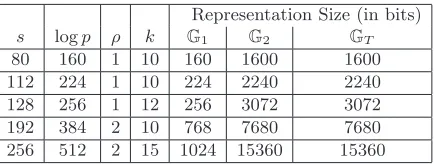
Figure 6: Group sizes for some pairing instantiations. Each value ofsrepresents a common security level for pairings. Here p is the common order of the groups, i.e. _|G_{1| = |}G_{2| = |}G_{T| = p. The} value ρ determines the size of the representation of an element in G_{1, where the size (in bits) is} ρ_·logp. Finally,kis the embedding degree and determines the size of the representation ofG_{2 and} G_{T, where the size (in bits) isρlogp}k_.

and using Equations(8) and (9) we have that

WF(_B) = T(A) +Tsim(n, q) ǫ2_{/(27nq+ 3ǫ)} =

(27nq+ 3ǫ)

ǫ · WF(A) +Tsim(n, q)·ǫ

−1 _{. (26)}

A security proof is only meaningful when the adversary it constructs has work factor less than that of the best known attack. Otherwise, the proof does not guarantee that finding a successful attacker against the scheme contradicts our confidence in the hardness of the underlying problem. Pollard’s rho algorithm for finding discrete logs in G_{1 is the best known attack against DBDH.} (Our instantiations will ensure that finding discrete logs inG_{T is no easier than in} G_{1.) The work} factor of Pollard’s algorithm ends up being

WF(_P) = T(P) ǫp

= (0.88

√_p·T

op(G1))2

T(_P) ≥0.88

√_p

·Top(G1).

where the last inequality is because _P achieves no more advantage after running for time 0.88√p_·

Top(G1). We therefore compare the efficiencies of the two reductions based on their ability to satisfy

WF(_BWa)≤WF(P) or WF(B)≤WF(P)

for various values ofWF(_A), ǫ,q, and concrete pairing parameters.

Pairing instantiations. In Appendix E we discuss the (complex) topic of instantiating pairings for various security levels. Since not all security levels have efficient instantiations [19, 18], we limit our attention to severalpairing setups that correspond to the security levels indicated (for private and public-key cryptography) by the NIST key schedule [31]. These setups and their corresponding instantiation sizes are listed in Figure 6.

Comparing the reductions. We are now ready to perform the comparison. Letκ= logWF(_A). The tables in Figure 7 show the pairing setupsW needed to ensureWF(BWa)≤WF(P) is satisfied

and the pairing setup sN needed to ensure WF(B)≤WF(P) is satisfied, for the indicated values

of κ,ǫ, and q. Shown also is the pairing setup required forBB1. Note that while one can evaluate

the equations everywhere, some combinations ofκ,ǫ, andq don’t actually make sense, for example

−ǫ+q_≥κ implies that the adversary spends all its time making oracle queries. We have marked such combinations with a∗_.

the two setups suggested by the reductions.

We can calculate the approximate (using conventions discussed in Appendix E) efficiency dif-ference for encryption whenWais instantiated with pairing setupsW versussN using the following

ratio

T_exp(G_{T) +}T_op(G_{T) +}T_exp(G_{2) +}T_exp(G₁₎

Texp(G′T) +Top(G′T) +Texp(G′2) +Texp(G′1)

.

HereGP= (G_1,G_2,G_{T, p,e, ψ) are the pairings as instantiated under setupsW andGP}′ _{= (}G′

1,G′2,

G′

T, p′,e′, ψ′) are the pairings as instantiated under setup sN. Figure 2 in the introduction shows

this ratio for somesW, sN pairs.

Acknowledgments

We thank Brent Waters for pointing out a bug in the proof of an earlier version of this paper. We thank Sarah Shoup for participating in early stages of this work. We thank Dan Boneh and Xavier Boyen for comments on earlier drafts of this work.

References

[1] M. Abdalla, D. Catalano, A. W. Dent, J. Malone-Lee, G. Neven, and N. P. Smart. Identity-based encryption gone wild. In M. Bugliesi, B. Preneel, V. Sassone, and I. Wegener, editors, ICALP 2006, volume 4052 ofLNCS, pages 300–311, Venice, Italy, July 10–14, 2006. Springer-Verlag, Berlin, Germany.

[2] M. Abdalla, E. Kiltz, and G. Neven. Generalized key delegation for hierarchical identity-based encryption. InESORICS, volume 4734 ofLecture Notes in Computer Science, pages 139–154. Springer, 2007.

[3] M. Bellare, C. Namprempre, and G. Neven. Unrestricted aggregate signatures. In L. Arge, C. Cachin, T. Jurdzi´nski, and A. Tarlecki, editors,ICALP 2007, volume 4596 ofLNCS, pages 411–422, Wroclaw, Poland, July 9–13, 2007. Springer-Verlag, Berlin, Germany.

[4] M. Bellare and P. Rogaway. The Security of Triple Encryption and a Framework for Code-Based Game-Playing Proofs. In S. Vaudenay, editor, EUROCRYPT 2006, volume 4004 of LNCS, pages 409–426, St. Petersburg, Russia, May 29 –June 1, 2006. Springer-Verlag, Berlin, Germany.

[5] J. Birkett, A. W. Dent, G. Neven, and J. C. N. Schuldt. Efficient chosen-ciphertext secure identity-based encryption with wildcards. In J. Pieprzyk, H. Ghodosi, and E. Dawson, edi-tors,ACISP 07, volume 4586 ofLNCS, pages 274–292, Townsville, Australia, July 2–4, 2007. Springer-Verlag, Berlin, Germany.

[6] D. Boneh and X. Boyen. Efficient selective-ID secure identity based encryption without random oracles. In C. Cachin and J. Camenisch, editors,EUROCRYPT 2004, volume 3027 ofLNCS, pages 223–238, Interlaken, Switzerland, May 2–6, 2004. Springer-Verlag, Berlin, Germany. [7] D. Boneh and X. Boyen. Short signatures without random oracles. In C. Cachin and J.

Ca-menisch, editors,EUROCRYPT 2004, volume 3027 ofLNCS, pages 56–73, Interlaken, Switzer-land, May 2–6, 2004. Springer-Verlag, Berlin, Germany.

[9] X. Boyen. General ad hoc encryption from exponent inversion IBE. In M. Naor, editor, EUROCRYPT 2007, volume 4515 of LNCS, pages 394–411, Barcelona, Spain, May 20–24 2007. Springer-Verlag, Berlin, Germany.

[10] X. Boyen, Q. Mei, and B. Waters. Direct chosen ciphertext security from identity-based techniques. In V. Atluri, C. Meadows, and A. Juels, editors, ACM CCS 05, pages 320–329, Alexandria, Virginia, USA, Nov. 7–11, 2005. ACM Press.

[11] R. Canetti, S. Halevi, and J. Katz. A forward-secure public-key encryption scheme. In E. Bi-ham, editor, EUROCRYPT 2003, volume 2656 of LNCS, pages 255–271, Warsaw, Poland, May 4–8, 2003. Springer-Verlag, Berlin, Germany.

[12] R. Canetti, S. Halevi, and J. Katz. Chosen-ciphertext security from identity-based encryption. In C. Cachin and J. Camenisch, editors, EUROCRYPT 2004, volume 3027 of LNCS, pages 207–222, Interlaken, Switzerland, May 2–6, 2004. Springer-Verlag, Berlin, Germany.

[13] S. Chatterjee and P. Sarkar. Trading time for space: Towards an efficient IBE scheme with short(er) public parameters in the standard model. In D. Won and S. Kim, editors,ICISC 05, LNCS, pages 424–440, Seoul, Korea, Dec. 1–2, 2005. Springer-Verlag, Berlin, Germany. [14] S. Chatterjee and P. Sarkar. HIBE with short public parameters without random oracle. In

ASIACRYPT 2006, LNCS, pages 145–160. Springer-Verlag, Berlin, Germany, Dec. 2006. [15] D. Chaum, J.-H. Evertse, and J. van de Graaf. An improved protocol for demonstrating

possession of discrete logarithms and some generalizations. In D. Chaum and W. L. Price, editors,EUROCRYPT’87, volume 304 ofLNCS, pages 127–141, Amsterdam, The Netherlands, Apr. 13–15, 1987. Springer-Verlag, Berlin, Germany.

[16] L. Chen and Z. Cheng. Security proof of Sakai-Kasahara’s identity-based encryption scheme. In N. P. Smart, editor, IMA Int. Conf., volume 3796 of Lecture Notes in Computer Science, pages 442–459. Springer, 2005.

[17] C. Cocks. An identity based encryption scheme based on quadratic residues. In B. Honary, editor, Cryptography and Coding, 8th IMA International Conference, volume 2260 of LNCS, pages 360–363, Cirencester, UK, Dec. 17–19, 2001. Springer-Verlag, Berlin, Germany.

[18] D. Freeman, M. Scott, and E. Teske. A taxonomy of pairing-friendly elliptic curves. Cryptology ePrint Archive, Report 2006/372,http://eprint.iacr.org/, 2007.

[19] S. D. Galbraith, K. G. Paterson, and N. P. Smart. Pairings for cryptographers. Cryptology ePrint Archive, Report 2006/165.http://eprint.iacr.org/, 2006.

[20] D. Galindo. The exact security of pairing based encryption and signature schemes. Based on a talk at Workshop on Provable Security, INRIA, Paris, 2004.http://www.dgalindo.es/ galindoEcrypt.pdf, 2004.

[21] C. Gentry. Practical identity-based encryption without random oracles. In S. Vaudenay, editor, EUROCRYPT 2006, volume 4004 of LNCS, pages 445–464, St. Petersburg, Russia, May 29 –June 1, 2006. Springer-Verlag, Berlin, Germany.

[22] M. Green and S. Hohenberger. Blind identity-based encryption and simulatable oblivious transfer. In K. Kurosawa, editor,ASIACRYPT 2007, volume 4833 of LNCS, pages 265–282. Springer-Verlag, Berlin, Germany.

[23] D. Hofheinz and E. Kiltz. Programmable hash functions and their applications. In D. Wagner, editor,CRYPTO 2008, volume 5157 ofLNCS, pages 21–38, Santa Barbara, CA, USA, Aug. 17– 21, 2008. Springer-Verlag, Berlin, Germany.

[24] J. Horwitz and B. Lynn. Toward hierarchical identity-based encryption. In L. R. Knudsen, edi-tor,EUROCRYPT 2002, volume 2332 ofLNCS, pages 466–481, Amsterdam, The Netherlands, Apr. 28 – May 2, 2002. Springer-Verlag, Berlin, Germany.

Press.

[26] E. Kiltz and D. Galindo. Direct chosen-ciphertext secure IB-KEM without random oracles. In L. M. Batten and R. Safavi-Naini, editors, ACISP 06, volume 4058 of LNCS, pages 336–347, Melbourne, Australia, July 3–5, 2006. Springer-Verlag, Berlin, Germany.

[27] A. K. Lenstra. Unbelievable security: Matching AES security using public key systems. In C. Boyd, editor, ASIACRYPT 2001, volume 2248 of LNCS, pages 67–86, Gold Coast, Aus-tralia, Dec. 9–13, 2001. Springer-Verlag, Berlin, Germany.

[28] A. K. Lenstra and E. R. Verheul. Selecting cryptographic key sizes. Journal of Cryptology: the journal of the International Association for Cryptologic Research, 14(4):255–293, 2001. [29] A. J. Menezes, P. C. van Oorschot, and S. A. Vanstone. Handbook of Applied Cryptography.

The CRC Press series on discrete mathematics and its applications. CRC Press, 2000 N.W. Corporate Blvd., Boca Raton, FL 33431-9868, USA, 1997.

[30] D. Naccache. Secure and practical identity-based encryption. Cryptology ePrint Archive, Report 2005/369, 2005. http://eprint.iacr.org/.

[31] National Institute for Standards and Technology. Recommendation for Key Management Part 1: General (revised), 2005. NIST Special Publication 800-57.

[32] J. M. Pollard. Monte Carlo methods for index computation (mod p), 1987. Mathematics of Computation, 32:918-924.

[33] T. Ristenpart and S. Yilek. The Power of Proofs-of-Possession: Securing Multiparty Signatures from Rogue-key Attacks. In M. Naor, editor,EUROCRYPT 2007, volume 4515 ofLNCS, pages 228–245, Barcelona, Spain, May 20–24 2007. Springer-Verlag, Berlin, Germany.

[34] A. Sahai and B. R. Waters. Fuzzy identity-based encryption. In R. Cramer, editor, EURO-CRYPT 2005, volume 3494 of LNCS, pages 457–473, Aarhus, Denmark, May 22–26, 2005. Springer-Verlag, Berlin, Germany.

[35] R. Sakai and M. Kasahara. ID based cryptosystems with pairing on elliptic curve. Cryptology ePrint Archive, Report 2003/054, 2003. http://eprint.iacr.org/.

[36] B. R. Waters. Efficient identity-based encryption without random oracles. In R. Cramer, editor, EUROCRYPT 2005, volume 3494 of LNCS, pages 114–127, Aarhus, Denmark, May 22–26, 2005. Springer-Verlag, Berlin, Germany.

A

Derivatives of Waters’ IBE

A large body of research [10, 1, 5, 26, 30, 13, 14, 22] utilizes Waters’ scheme. Recall that Waters’ already proposed a heirarchical IBE scheme based on Wa in [36], and subsequently there have been numerous derivative works. All use the artificial abort, either due to a black-box reduction to Waters’ (H)IBE or as an explicit step in a direct proof. Our new proof technique immediately benefits those schemes that utilize Waters’ scheme directly (i.e. in a black-box manner). For the rest, we believe that our techniques can be applied but have not checked the details.

• Naccache [30] and Chatterjee and Sarkar [13, 14] independently and concurrently introduced a space-time trade-off for Wa that involves modifying the hash function utilized from H(u, I) =

u[0]Qn_i=1u[i]I[i] _{for u ∈ G}n+1

1 to H′(u, I) = u[0]

Qℓ

i=1u[i]I[i] where u ∈ Gℓ1+1 and each I[i] is

now an n/ℓ-bit string. For appropriate choice of ℓ this will significantly reduce the number of elements included in the master public key. However the new choice of hash function impacts the reduction tightness, and since their proof includes just minor changes to Waters’, our new reduction will increase the efficiency of this time/space trade-off for various security levels.

• In [10]BB1- andWa-based constructions of CCA-secure public-key encryption schemes and their

• Kiltz and Galindo [26] propose a construction of CCA-secure identity-based key encapsulation that is a modified version of Wa.

• Wildcard IBE [1, 5] is a generalization of heirarchical IBE that allows encryption to identities that include wildcards, e.g. “*@anonymous.com”. In [1] a wildcard IBE scheme is proposed that utilizes the Waters HIBE scheme, and the proof is black-box to it. In [5] a wildcard identity-based KEM is produced based (in a non-black-box manner) on Waters’ IBE.

• Wicked IBE [2] allows generation of private keys for wildcard identities. These private keys can then be used to generate derivative keys that replace the wildcards with any concrete identity string. They suggest using the Waters’ HIBE scheme to achieve full security in their setting.

• Blind IBE, as introduced by Green and Hohenberger [22], enables the “trusted” master key gen-erator to generate a private key for an identity without learning anything about the identity. To prove a Waters’-based blind IBE scheme secure they utilize the Naccache proof [30] (mentioned above). They utilize blind IBE schemes to build efficient and fully-simulatable oblivious transfer protocols based on the assumptions inherited from the BDH-based IBE schemes used.

B

Proof of Lemma 2.1

We prove the lemma utilizing a coin-counting argument, following the approach of [4, Lemma 1]. For a pair of gamesGand Hand an advsersary_Awe assume that the number of random selection assignments s_←$ S is less than or equal to some number b_≥0 and each set S sampled from is of size less than or equal to d >0 (for simplicity we disallow empty sets). Then we define the coins for (G,H,_A) to be the set C = [0.. d!]b_{. Using coins c= (c}

1, . . . , cb)∈C, the ith random selection

statement s _←$ S = _{s1, s2, . . . , sm} for m < d in GA (equivalently HA) is executed by assigning

tosthe valuescimodm. (Note that there is no distinction between random assignment statements

in the game or the adversary, they are treated the same.) Since m divides d, then selecting c

uniformly ensures that each random assignment statement returns an indendently and uniformly chosen element from the set. We write GA(c) to denote running GA on the particular choice of coinsc.

LetCbe the set of coins for (G,H,_A) where G andH are identical-until-badgames and_Ais an adverary. LetGD_G (resp. GDH) be the event that badis not set in game G (resp. H). LetCG0=

{c_∈C : GA(c)_⇒y_} and CG1 =C\CG0. Let CGgood ={c∈C : GA(c) does not setbad}. Let

CGgood_k =CGgood_∩CG

k fork∈[0,1]. DefineCH0,CH1,CHgood, andCHkgood in the natural way.

Because G and H are identical-until-bad we have thatCGgood₁ =CH₁good. This is true because any vector c_∈CGgood₁ does not causebad to be set, thereby only code that is common with H is executed. So if GA(c)_⇒y then HA(c)_⇒y, makingc_∈CH₁good. A similar argument works in the other direction. So we have that

PrGA_⇒1_∧GD_G= |CG

good

1 |

|C_| =

|CH₁good_|

|C_| = Pr

HA _⇒1_∧GD_H.

C

Proof of Lemma 3.2

As per the lemma statement, let (g1, g2, A2, A1, B2, B1,x,y,u, S, W) be simulation parameters. For

aand b be the discrete logs (base g1) of A1 and B1, respectively. Define the functionf: Zp →Zp

by f(r) =r₋wamodp for allr _∈Z_{p. Now we claim that for any r∈}Z_{p we have}

Ab₁H(u, I)f(r) = B₁F(x,I)·rg₁G(y,I)·rA₁−G(y,I)·w (27)

gf₂(r) = g₂rA−w₂ (28)

In other words, the output ofKgS(g1, g2, A2, A1, B1,x,y, I) when r is the underlying randomness

equals the output of Kg(mpk, msk, I) when f(r) is the underlying randomness. But f is a per-mutation over Z_{p, so if r is uniformly distributed, so is f(r). This proves that the outputs of}

Kg(mpk, msk, I) and KgS(g1, g2, A2, A1, B1,x,y, I) are identically distributed as claimed. Let us

now verify equations (27) and (28). We have:

Ab₁H(u, I)f(r) = Ab_1· u[0]_·

n Y

i=1

u[i]I[i]

!r−w·a

= gab_{1 ·} B₁x[0]gy₁[0]_·

n Y

i=1

B₁x[i]I[i]g₁y[i]I[i]

!r−w·a

= B₁a_·B₁F(x,I)_·gG₁(y,I)r−w·a

= B₁a_·B₁F(x,I)·r_·B₁−a_·gG₁(y,I)r_·g₁−aG(y,I)·w = B₁F(x,I)·r_·g₁G(y,I)r_·A−G₁ (y,I)·w.

We know thatg1 =ψ(g2) andA1=ψ(A2) =g1a. This means that A2 =g2a. So

gf₂(r)=g₂r−w·a=gr₂A−w₂ ,

which completes the proof of the first part. For the second part, we assume that F(x, I) = 0 and let (C1, C2, C3)←EncS(S, W, M,y, I). Letsbe the discrete log ofS to baseg2. ThenC1 =W·M;

C2=S; and using thatψ(S) =g1s we have

C3 =ψ(S)G(y,I)= (g1s)G(y,I)=

g₁G(y,I)s=B₁0g₁G(y,I)s=B₁F(x,I)g₁G(y,I)s=H(u, I)s. Thus (C1, C2, C3) is exactly (W·M, S, H(u, I)s).

D

Proof of Lemma 3.5

Fix an arbitrary (I0, . . . , Iq)∈ID. We will show that

1 n(m₋1) + 1

1₋ q m

≤ γ(I0, . . . , Iq) (29)

1

The lemma follows. We first prove (29). We stress that below (I0, . . . , Iq) ∈ ID is fixed and the

probability is only over the random choice ofxfromX. LetEi be the event thatF(x, Ii) = 0. Then

1₋γ(I0, . . . , Iq) = Pr

E0∨E1∨ · · · ∨Eq

= PrE0∨(E0∧E1)∨ · · · ∨(E0∧Eq)

= PrE₀+ Pr [ (E_0∧E₁)_{∨ · · · ∨}(E_0∧Eq) ] (31) ≤ PrE0+

q X

i=1

Pr [E0∧Ei] (32)

For every choice of x[1], . . . ,x[n] there is exactly one choice of x[0] such thatF(x, I0) = 0, so that

Pr [E₀] = 1

n(m₋1) + 1. (33)

Now let i_∈[1.. q]. SinceI0 6=Ii there is aj∈[1.. n] such thatIi[j]6=I0[j]. Let s∈ {0, i}be such

thatIs[j] = 0 and Ii−s[j] = 1. For any choice ofx[1], . . . ,x[j−1],x[j+ 1], . . . ,x[n] let

t0 =−

X

l6=j

x[l]Is[l] and tj =−t0−

X

l6=j

x[l]Ii−s[l].

Then F(x, I0) and F(x, Ii) are both zero only if (x[0],x[j]) = (t0, tj). Since x[0] is drawn from

[₋n(m₋1)..0] andx[j] from [0.. m₋1] this means that Pr [E0∧Ei]≤

1

n(m₋1) + 1· 1

m. (34)

One might ask why (34) is an inequality rather than an equality; isn’t the probability that (x[0],x[j]) equals (t0, tj) exactly the term on the right? The reason it is not is thattj may not lie in [0.. m−1],

so for some choices of the other coordinates ofx, the probability that x[j] =tj is zero.

Putting together (32), (33), and (34) we have 1₋γ(I0, . . . , Iq) ≤ 1−

1

n(m₋1) + 1+

q X

i=1

1 m ·

1

n(m₋1) + 1 = 1−

1 n(m₋1) + 1

1₋ q m

which implies (29).

To derive (30), we note that (31) implies that 1₋γ(I0, . . . , Iq) ≥Pr

E0 which, when combined

with (33), implies (30).

E

Instantiating Pairing Parameters

Pairings and their costs. LetGP= (G_1,G_2,G_{T, p,e, ψ) be pairing parameters as per Section 2.} We focus on the Type 2 [19] setting for these parameters, since the Type 1 (i.e., the symmetric setting where G_{1 =} G_{2) is not easily instantiated for higher security levels [19]. In the Type 2} setting, G_{1 is a subgroup of E(}F_{r) where} F_{r is a finite field. Group} G_{2 is a subgroup of E(}F_rk)

where k is called the embedding degree. Group G_{T is a subgroup of} F∗

rk. All three groups G1, G_{2, and}G_{T are of order p for some prime p that divides r}k_{−1. Let ρ= (logr)/(logp), which we} call the representation multiplier. Elements of G_{1 require ρlogp bits to represent while elements} of G_{2 and} G_{T require kρlogp bits to represent. We fix the following conventions regarding the} computational costs of basic operations related to an instantiation of GP.