VICTORIA
~ UNIVERSITY+;
DEPARTMENT OF COMPUTER AND
MATHEMATICAL SCIENCES
Model of Process Control System Applied
to Product Quality
Venkatesan Gopalachary
87 STAT 4
May 1997
TECHNICAL REPORT
VICTORIA UNIVERSITY OF TECHNOLOGY
P 0BOX14428
~LBOURNE
CITY MC
VIC 8001
AUSTRALIA
MODEL OF PROCESS CONTROL SYSTEM
APPLIED TO PRODUCT QUALITY
VENKATESAN GOPALACHARY
Department of Computer and Mathematical Sciences, Victoria University of
Technology, PO BOX 14428MCMC, Melbourne 8001, Australia
ABSTRACT
This paper is aimed at finding a solution to the commonly occurring product quality control problem by suitably modelling a process control system. The techniques from engineering and statistical process control overlap at the interface of the two process control methodologies. Problems connected with feedback (closed-loop) stability, controller limitations and dead-time compensation to obtain minimum variance (mean square) control at the output are encountered while applying statistical process monitoring and feedback control adjustment. The focus in this paper is to model a control system by application of both the process control techniques.
1 INTRODUCTION
assessment of control loop performance, on-line process control, discrete stochastic and
linear quadratic controllers etc. These contributions, along with the work done
independently by control engineers in automatic process control, focus only on
particular aspects of process control. This paper is in the direction of modelling a
process control system applied to product quality.
2 STOCHASTIC DISTURBANCE MODEL AND FEEDBACK CONTROL
DIFFERENCE EQUATION
APC aims to maintain certain key process variables as near their set points
(targets) for as much of the time as possible in order to satisfy certain production
objectives. One of the production objectives is to produce material of desired quality by
having an acceptable level of variation (product variability) in the measured output
characteristics. Disturbance (noise) causes variability in the output or outputs of an othenvise stable process by producing undesirable changes in the (output) mean.
Disturbances cause a process to wander and drift off target resulting in shifts in the
mean of the output product quality away from target. The error, the difference between
the output and target values, is used to determine a process adjustment. If no
compensatory adjustments are made and no (feedback) control actions are taken, the
output follows the course of the disturbance. The effect of an input adjustment (control
action) is delayed in its effect due to dead time, (time taken to deliver material from the
point of adjustment to the sample point), in the process. The presence of dead time in
the process requires that forecasts of the output deviation (error) are made over the delay
period.
An ARIMA (Autoregressive integrated movmg average) model is used to
forecast the behaviour of the time series describing the disturbance. The integrated
moving average model has the property that the forecasts for all future time is an
exponentially weighted moving average (EWMA) of current and past values of the
disturbance. The EWMA provides the forecasts over the dead time period (time delay).
Moreover, the time series controller gives (b+ 1) periods ahead forecast error variances over the time delay (dead time) period in a process.
The ARIMA (0, 1, 1) stochastic time series model characterising the drifting
(1)
where 'z' is the stochastic variable and 'at', the random variable. Z' represents the stochastic disturbance and { 3t} represents the sequence of random variables.
Zt,
is the output of a (linear) process control system, when subjected to a sequence of uncorrelated random shocks {at}, where at follows a Normal distribution with mean 0and standard deviation cra, represented by at -N(O,cra2).
e
is the integrated movingaverage (IMA) parameter.
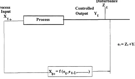
Figure 1 describes the relationship between the output (Y t) and the input (Xt+) in the feedback control model.
Process In put
xt+
c
ontro e II d OutputProcess
x t+ = f ( e ,e _ , ... ) t t 1
Disturbance
zt
yt
Figure 1 Block Diagram for the Feedback Control Model
et= Zt +Yt
The 'stochastic difference equation' for the feedback control model can be
(approximately) represented by the following second-order dynamic model (transfer
function) of the
form:-Yt (1- 81B - 82B2) = roBb+l Xt, (2)
where
Xt+, the input put manipulative variable, is a linear function of~, the forecast error and
of integral over time of past errors,
81 and 82 are the parameters that represent the dynamics (inertial) characteristics of the
system, Bis the backward shift operator; BXt = Xt-J, BbXt= Xt-b·
co is the magnitude of the process response to a unit step change in the first period
following the dead time carrying over into additional sample periods.
b is the process dead time, b > -1. PG represents the process gain realised by total effect
in output caused by a unit change in the input variable after the completion of the
dynamic response.
et; is the forecast error in Figure 1 and~= Zt+Yt.
It can be shown that (i) PG = l/(l-81-82) = g, the steady-state gain for a critically
damped second-order dynamic system when the conditions given below are satisfied
and (ii) co= PG(l-81-82) =lfor a critically damped system.
Equation (2) describes the critically damped behaviour of the second-order dynamic
system for which the time constants are real and equal. The following inequality
conditions are imposed for closed-loop stability.
81+82<1,
82-81 <1,
-1<82<1,
812+482 = 0.
3 EXPRESSION FOR FEEDBACK CONTROL ADJUSTMENT
From Equations (1) and (2) for the stochastic and dynamic models, an
expression for feedback control adjustment is developed which minimizes the variance
of the output controlled variable by making an input control adjustment at every sample
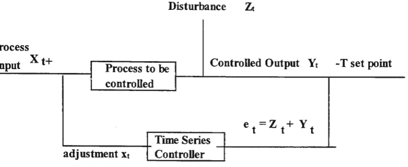
point that exactly compensates for the forecasted disturbance. Figure 2 shows a
feedback control scheme to compensate disturbance in a second-order dynamic model
with delay (dead time). Refer to Venkatesan [1995] for derivation of the feedback
Disturbance Zt.
Process
Input Xt+ Process to be Controlled Output Yt -T set point
controlled
et=Zt+Yt Time Series
adjustment Xt Controller
Figure 2 Feedback Control scheme to compensate disturbance Zt.
(3)
This feedback control algorithm gives information about when to make an
adjustment and by how much. The control adjustment given by Equation (3) minimises
the variance of the output controlled variable even in the face of dead time (time delay)
and process dynamics (inertia).
The first term in the above stochastic feedback control algorithm represents the
integral term and the second term, the dead-time compensator developed by Smith
[1959] (Baxley [1991]). According to Palmor and Shinnar [1979], the Smith predictor is
a direct result of minimal variance strategy and that minimal variance control for
processes having dead times includes this type of dead-time compensation. At this stage,
an intuitive conjecture is made that the inclusion of the dead-time compensation term of
either the Smith predictor or the Dahlin's (on-line) tuning parameter, (whose values
range from 0 to 1 ), in a feedback control algorithm will also result in a minimum
variance strategy for processes with dead time.
This draws on the comparison made by Harris, MacGregor and Wright [1982] to
the minimum variance controller they derived for the process with dead time (for which
the number of whole periods of delay was equal to 2) and the Dahlin controller (Harris,
MacGregor and Wright [1982]) given in their paper. The authors showed that the two
time constant of the closed-loop process), equal to 0, the IMA parameter in the
stochastic disturbance model. They reconciled the different approaches by noting that
the 'IMA parameter 0 provides information about the magnitude of the closed-loop time
constant'.
Equation (3) is identical to Baxley's [1991] algorithm for a first-order model
with dead time and includes both integral action and dead-time compensation terms,
when
ch=
0 and 01= o
and b =1. The control obtained through the first term in Equation(3) is the discrete analogue of integral control. The IMA parameter 0, (whose values
range from 0 to 1), is set to match the disturbance as well as take care of Dahlin's
parameter to compensate for the dead time. It is used as an on-line tuning parameter for
dead-time compensation. So, it follows that the variance of the output product variable
achieved by using Equation (3) with integral action and dead-time compensation terms
is a minimum. The dead-time compensation term (seemingly) removes the delay from
stability considerations and definitely provides a stabilising effect on the feedback
control system. These principles are used for designing (formulating) the discrete
(sampled-data) time series controller. Such a controller will maintain the mean of the
process quality variable at or near target and will allow for a (rapid) response to process
disturbances without much overcompensation or overcorrection.
4 SIMULATION AND ANALYSIS
The stochastic feedback control algorithm is simulated to firtd the time series
controller performance measures, namely, CESTDDVN (control error standard
deviation) or control error sigma (product variability) and the mean frequency of
adjustment (MFREQ) of the time series controller. An advantage of dead-time simulation is that the inter-sample variances are compared at the sampling points. Table
1 gives the control error sigma (CESTDDVN) and the mean frequency of adjustment
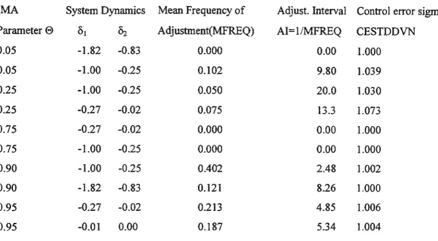
Table 1 Time series Controller Performance Measures
---IMA System Dynamics Mean Frequency of Adjust. Interval Control error sigmaParameter 0 01 02 Adjustrnent(MFREQ) AI=l/MFREQ CESTDDVN
0.05 -1.82 -0.83 0.000 0.00 1.000
0.05 -1.00 -0.25 0.102 9.80 1.039
0.25 -1.00 -0.25 0.050 20.0 1.030
0.25 -0.27 -0.02 0.075 13.3 l.073
0.75 -0.27 -0.02 0.000 0.00 1.000
0.75 -1.00 -0.25 0.000 0.00 l.000
0.90 -1.00 -0.25 0.402 2.48 1.002
0.90 -1.82 -0.83 0.121 8.26 1.000
0.95 -0.27 -0.02 0.213 4.85 1.006
0.95 -0.01 0.00 0.187 5.34 1.004
The above table shows a range of minimal control error sigmas (CESTDDVN)
for values of 0 and the dynamic (inertial) parameters 8i, 82. The values of
CESTDDVNs are 1.0, when 0 = 0.75, the EWMA forecasts are effective and the
EWMA has good control of the process. Since the CESTDDVN values, (close to around
the value of 1. 0), are obtained for the second-order dynamic process with dead time b =
1, it is possible to achieve good (feedback) control possessing features such as (i)
Permissible gain of the feedback (closed) loop, (ii) Stability of the feedback control loop
and (iii) Precise regulation of loops containing dead time. The range of control error
sigmas (CESTDDVN) for corresponding values of 0 can be used to formulate process
regulation schemes. These values of 0 and AI are used to formulate process regulation
schemes as shown in the next Section.
A dead-time compensation scheme which provides a process gain (PG) in the
feedback path whose value depends on both the process output and model has been
devised This scheme is suited to use in situations where the process dead time results
from a measurement device in a laboratory and is a known quantity. A process
modelling (control) approach to product quality based on discrete laboratory data has
the potential for improvements (in product quality). A practical control strategy would
then be (i) based on the use of quality control laboratory analyses and (ii) the process
closed-loop experiment and using the laboratory data to update the set point of the minimum
variance time series controller to verify the quality of outgoing product.
5 PROCESS REGULATION SCHEMES
The choice of feedback control process regulation schemes depends on 'how
capable' the 'controlled process' (model) was of providing quality products within
manufacturing specifications. If the process capability index was high, then, a moderate
increase in the control error deviation (product variability) might be tolerated if this
action resulted in savings in sampling and adjustment costs. Table 2 shows the
adjustment interval (AI) and the corresponding CESTDDVN for some alternative
schemes using combinations of control limits L = 2.98, 3.0 and 3.04. These schemes are
denoted by A, B, ... 0. These schemes are based on how much the CESTDDVN would
need to increase to achieve the advantage of taking samples and making adjustments
less frequently. This approach avoids the direct assignment of values to costs Ca (cost of
adjustment and sampling) and C1 (cost of being off-target). The table 2 shows for
various values of the standardised action limit, L/cra = 3.010, 3.000, 3.009 and the
adjustment interval (AI), the percent of increase in CESTDDVN (ISTD.) with respect to
cra and AI. The AI and CESTDDVN values show that for different sets of values of AI
and CESTDDVN, the process regulation scheme varies according to the AI values.
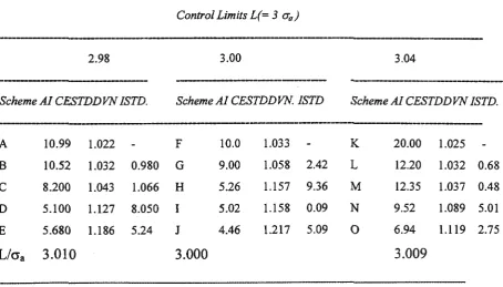
Table 2 Alternative Process Regulation Schemes
Control Limits L(= 3 a0 )
2.98 3.00 3.04
---Scheme AI CESTDDVN !STD. Scheme AI CESTDDVN. !STD Scheme AI CESTDDVN /STD.
A 10.99 1.022 F 10.0 1.033 K 20.00 1.025
B 10.52 1.032 0.980 G 9.00 1.058 2.42 L 12.20 1.032 0.68
c
8.200 1.043 1.066 H 5.26 1.157 9.36 M 12.35 1.037 0.48D 5.100 1.127 8.050 I 5.02 1.158 0.09 N 9.52 1.089 5.01
E 5.680 1.186 5.24 J 4.46 1.217 5.09 0 6.94 1.119 2.75
The alternative schemes are: (i) Scheme B: To set L = 2.98 and adjust process at
10.5 sample periods, with an increase in CESTDDVN (ISTD.) of 0.98 or
(ii) Scheme E: Adjust process at 5.7 sample periods and ISTD of 5.24 or (iii) Scheme J:
by setting L = 3.0 and AI= 4.46 sample periods, the same ISTD. could be achieved with
an AI of 4.5.
6 ENGINEERING CONTROL APPLICATION TO PRODUCT QUALITY
To control the quality of a product at the output, the set point of a
product-quality controller is adjusted so that the product remains within its specification limits
following expected load changes or disturbances. In product quality control, the
product-quality set point is adjusted away from the specification limit in proportion to
the peak deviation expected to be yielded by the controller. Again, the adjustment is in a
direction that increases operating costs. Deviation in the 'safe' direction increases
operating costs in proportion to the deviation. The quality-controller's set point is
positioned relative to the specification limit so that the limit will not be violated for
most upsets (load changes). Since the average output product quality will be equal to the
set point, the product will be more expensive to make than if the set point were
positioned exactly at the specification limit. Excess manufacturing cost is proportional
to the difference between the set point and the specification limit and so, proportional to
the peak deviation expected. By limiting the peak deviation, excess manufacturing cost
and product quality are controlled in engineering control. Peak deviation of the
controlled variable from set point is significant when excessive deviation will cause an
incident such as rejecting product due to failure to meet specifications.
Process control provides the operating conditions under which a process will
function safely, productively and profitably. Ineffective control can be costly in causing
amongst other things such as plant shutdown, in allowing off-specification product to be
made, etc. For a particular control loop, it is often possible to relate operating cost to
deviation of the output controlled variable. In product-quality control loop, the cost
function is usually found to be different on opposite sides of set point.
Process operators frequently place a large margin between the measured quality
of a product and its specification. This is done in order to counteract the changes in
economic performance when a product specification is violated. It will cost more to
meets exactly the specifications; but variations in product quality are not equally
acceptable on both sides of the specification. So, as a consequence, the quality set point
must be positioned far enough without excessive operating costs, on acceptable side of
the specification in order to reduce the likelihood of specification violation. The
operating cost can be reduced by better control and smaller variation in quality allowing
the set point to be moved to closer the specification.
The deviation between the output controlled variable and its set point can be
related (linearly) to operating cost. For a specific production rate, each increment of
time will correspond to a quantity of product manufactured over that time. So,
integration of deviation (error) over time could be equated to accumulated (excess)
operating cost. Under such circumstances, the control objective would be to minimize
integrated error*. This criterion could be applied to control the quality of a product
flowing into a storage tank, for example. This can be achieved by keeping the integrated
error as low as possible and the quality of the product closer to the set point. *Integrated
error can be estimated from the feedback control equation (3), being equal to
(ei-81ei-1-82ei-2). It is a function of the change required in the input manipulated variable
and the setting of the integral mode of the (time series) controller. Integrated error can
be significant in product-quality loops, where it may represent excessive operating cost
such as product giveaway. Lag-dominant dynamics characterize, (similar to the
second-order dynamic model with two exponential terms), most of the important plant loops
such as product quality. For these processes, the integral error varies linearly with time.
7 STATISTICAL QUALITY CONTROL APPLICATION TO PRODUCT
QUALITY
For the sample values of a product variable whose measurements are normally
distributed, its mean will equal the set point if the integral of the error approaches zero
over a period of time. In minimizing the deviation of the output controlled variable, the
standard deviation is a transformation of that deviation over a statistically significant
number of samples or time of operation. The economic incentive behind the
standard-deviation criterion is that this criterion estimates the percentage of time the controlled
variable violates the specification based on a normal distribution. If samples of an
to form a subgroup, then the mean of subgroups will lie on the set point and their
standard deviation will approach zero (if there are no disturbances in the feedback
control system).
The assignment of subgroup size should reflect the capacity of a process to
absorb variations in product quality. The method used to average samples also needs to
be selected to match the characteristics of the process. If the product is segregated into
lots, then, the samples should be segregated into the same lots and averaged equally.
Different criteria can be applied to set point and load disturbances that affect a
control loop. Different controller settings will be required to satisfy these criteria.
Overshoot of the output controlled variable can be minimized by limiting the rate of the
set-point changes that are likely to be introduced by the operator during the course of
plant operation and process control.
8 CONCLUSION
In this paper, the objective of applying the engineering and statistical techniques
to find a solution to the product quality control problem was explained. Techniques
from the two different disciplines at the interface of the two process control
methodologies were used to derive a feedback control difference equation and an
expression for feedback control adjustment. An analysis of simulated results were given
and also some process regulation schemes along with engineering and statistical control
REFERENCES
(1) Baxley, Robert V, (1991). A Simulation Study Of Statistical Process Control
Algorithms For Drifting Processes, SPC in Manufacturing, Marcel Dekker,
Inc., New York and Basel.
(2) Harris, T.J., MacGregor, J.F. and Wright J.D., (1982). An Overview of
Discrete Stochastic Controllers: Generalized PID Algorithms with Dead-Time
Compensation, Can. J. Chem. Eng. 60, 425-432.
(3) Palmor Z.J. and Shinnar R., (1979). Design of Sampled Data Controllers,
Industrial and Engineering Chemistry Process Design Development,
Vol.18, No.I, 8-30.
(4) Venkatesan G., (1995). A Feedback Control Algorithm for A Second-Order
Dynamic System, Department of Computer and Mathematical Sciences,