Optimization of Quicklime Production from
Snail Shell using Factorial Analysis Method
* Akande Funsho, Hassan, Yusuf Kehinde Mudi, and Kefas, Ephraim Gaska
Department of Chemical Engineering, Kaduna Polytechnic, Kaduna, PMB 2021, Kaduna Nigeria. * Corresponding author: E-mail: 38TU[email protected]U38T Phone number: 08033686645
Abstract
A snail shell, which is primarily composed of calcium carbonate, was thermally decomposed to produce quicklime. The effects of three calcination process variables (calcination temperature, calcination time and snail shell particle size) on quicklime yield were investigated using the design of experiment factorial analysis method. A replicated full factorial experiment was conducted to evaluate the interaction and main effects of these calcination process variables on quicklime yield. Optimal quicklime yield of 94.9663% was obtained at optimum conditions of; calcination temperature, 900 oC, calcination time, 150 min and snail shell particle size, 0.1 mm. the results of the analysis also revealed that there is a significant interaction between calcination temperature and particle size to produce quicklime of high yield.
Keywords: factorial analysis, optimization, snail shell, quicklime, calcination
1. Introduction
Snails belong to the family of phylum mollusks or mollusks and to the class gastropods, a large
group of invertebrate animals, mostly found in wet vegetation in damp and shady places, especially during rainy seasons [1]. Snails have a single usually spirally coiled shell, into which the body can withdraw when the snail’s body is drawn into the shell, it is sealed by a Horney plate called the operculum.
The main constituent of the snail shell is calcium carbonates which are either of two crystalline forms calcite and aragonite. The remainder is organic matrixes which constitute a protein known as conchiolin that usually makeup to 5% of the shell [2]. Calcium carbonate (CaCOR3R), the
primary raw material in the production of quicklime accounts for about 98% of the total composition of the Snail Shell. [3]; [4]; [5]. It is, therefore, indicated that Snail Shells have the same primary composition as calcium compounds. On the basis of the common compositional characteristics of Snail Shells, it was reasoned in this study that the calcination of the Snail Shells could produce high-quality quicklime. Consequently, the calcination of Snail Shell, with a focus on determining the settings of calcination parameters that will simultaneously optimize quicklime yield and quality with minimal variation will be investigated [5]. If this study is carried out, a means of safely and economically disposing of the Snail Shells would have been found and could also help in producing quicklime of high quality.
Several researchers have carried out researches on snail shell as a source of quicklime. One of the various studies includes [6], who studied the effect of Snail shell characteristic properties and calcination temperature on lime quality as well as the reactivity of the laboratory and
industrial limes from snail shells. He affirmed from his study that by the middle of the 19th century, the process of lime production changed and launched the used of modern vertical and rotary lime kiln instead of the old traditional lime kiln. His study also revealed that quicklime of high quality was produced from Snail shell via conversion of calcium carbonate to calcium oxide and quicklime which needed to be stored in airtight silos because the chemical is very susceptible to moisture. This result is in line with the reported work of [7] and [3] who independently studied the effects of Snail shell characteristics and calcination temperature to the reactivity of the quicklime. Two Snail shell samples from Sises (LRsR) and Latzima (LRLR) were
calcined at four different temperatures 900 P
o
P
C, 1000 P
o
P
C, 1100 P
o
P
C, and 1200 P
o
P
C. The analysis of the quicklime produced after was carried out by mercury intrusion porosimetry and nitrogen adsorption. The result of their studies revealed that the physical and chemical properties of lime vary considerably depending upon the Snail-shell from which it was derived. These were confirmed because the total cumulative volume, total porosity, and specific surface area of the quicklimes obtained from the two snail shells varies.
Other researchers who worked on the characteristics of quicklime production from snail shells include [8] who studied the effect of the fillers flow index, ultimate stress and strains on the tensile modulus of conducting resins using two-level factorial design. The result of their analysis shows that the three main factors have a significant effect on the tensile modulus of conductive resins. Also, [9] investigated the effect of lime content on Hot Mix Asphalt (HMA) stripping and grading using the Design of Experiment (DOE). In their study, DOE was used to study the effect of grading and lime content on the dry and saturated indirect tensile strength of HMA. They used the linear, quadratic and interactive terms of the factors to examine their developed models and fitting them to the experimental result. Their result shows that maximum tensile strength ratio was achieved at when lime content and with grading containing most coarse aggregate was used.
There are several experimental strategies that can be used when planning a test series. [10] described the factorial design as a strategy where the variables are simultaneously varied instead of varying One Variable at a Time (OVAT). One big advantage is that it considers interactions between the factors. A factorial design is, in other words, said to be a suitable method to examine if a factor has an influence on a specific variable or not [10] writes that in a factorial design, each level of the variables is studied for each complete replication of the experiment for all possible combinations.
[11] studied the optimization of the production of quicklime by calcination in rotary kilns. The limitation of their study is that the degree of the influence of the calcination process variables and the significance of their interaction on quicklime yield were not investigated. Also, the empirical model developed in their study does not include a significant variable, Snail shell composition. Qualitative model validation by justifying the behaviour of the output response (yield) and properties (microstructures and surface area) with respect to the variation of input variables, based on published work by researchers and practitioners in this field were not carried out. This premise the need to further study factorial analysis of quicklime production from Snail shell.
2. Materials and Methods
2.1 Sample preparation
The Snail shell used as a raw material for this research were obtained from dump sites and market in Kaduna State, Northern Nigeria. They were repeatedly washed to remove dirt and other impurities, material, and subsequently dried under the sun. The dried Snail shell was crushed in a Jaw Crusher where the particle size was reduced to about 2 – 4 cm diameter after which the Snail-shell was ground to very small particle size and sieved into different particle sizes (80 4T, 100
2000 4Tfor effective study. The 450 was weig
with a temperature of 900 P
o
P
C for about 150 min.
2.2 Factorial Analysis Methodology
The factorial analysis method was used to determine the influence of process variables such as the calcination temperature, calcination time and particle size of the snail shell on the yield of quicklime. Minitab 17 software was used for implementing the factorial analysis methodology and analysis of results.
2.3 Factorial analysis experimental matrix determination
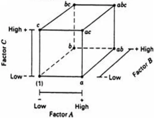
The geometric and experimental designs of the factorial analysis are shown in Figure 1 and Table 1 respectively.
Fig 1. Geometric design of three factors at two level settings
where
- represents the low-level setting + represents the high-level setting Factor A = Temperature = 𝑥1
Factor B = Time = 𝑥2 Factor C = Particle size = 𝑥3
The number of experimental runs required for the factorial analysis experimental matrix was determined using Equation (1)
No of Experimental Run = (𝐿𝑁)𝑅 = (23)2 = 16 (1)
The settings for the low and high levels for the calcination parameters is shown in Table1 were determined from the methodology of section 3.3.
Table 1: Coded Levels of the Independent Variables for the Low and High-Level Settings
Process Variables Low-level settings High-level settings
- +
XR1R: Calcination Temperature (P
o
P
C) 600 900
XR2R: Calcination Time (min) 30 150
XR3R: Snail shell Particle Size (mm) 0.1 0.45
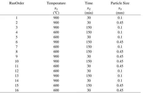
The factorial analysis experimental design matrix for the three factors and each of the sixteen experimental runs were generated using Minitab 17 software and the result is shown in Table 2.
Table 2: Experimental Design Matrix for Factorial Analysis Uncoded Factors
RunOrder Temperature Time Particle Size
𝑥1 𝑥2 𝑥3
(P
o
P
C) (min) (mm)
1 900 30 0.1
2 900 30 0.45
3 900 150 0.1
4 600 150 0.1
5 600 30 0.1
6 900 150 0.45
7 600 150 0.1
8 600 150 0.45
9 900 30 0.45
10 900 150 0.45
11 600 30 0.45
12 600 30 0.1
13 900 150 0.1
14 900 30 0.1
15 600 150 0.45
16 600 30 0.45
2.4 Calcination experiment methodology for quicklime yield determination
The calciner (carbolite furnace) was heated up to its starting temperature. 20 g of 0.1 mm (Run 1 snail shell particle size) snail shell sample was weighed in an electric weighing balance using ceramic crucible. The furnace door was opened and swung clear of the work tube to allow the ceramic crucible containing 20 g of 0.1 mm snail shell to be placed in the calciner. The calciner was powered on from the electric socket and the temperature controller knob was set to 900 P
o
P
C (Run 1 temperature). The calciner was allowed to heat up to the set soaking time of 30 min (Run 1 calcination time) and a calcination temperature of 900 P
o
P
C. The calciner was powered off and the door of the furnace was opened and tong was used to remove the sample in the crucible and transferred to a desiccator where the calcined snail shell was cooled down to room temperature. The snail shell sample was removed from the desiccator and put on a weighing balance to determine the weight of the snail shell sample. This was repeated for other runs (run 2-16) in the experimental matrix as shown in Table 2.
2.5 Factorial analysis experimental matrix quicklime yield determination methodology
The yield of calcined snail shell (quicklime) produced was determined according to ASTM C25.19 using Equation (2) For each varied calcination temperature, the loss on ignition and the yield of the quicklime produced from calcination experiment were calculated using Equations (2) and (3) respectively. The loss of mass on ignition (LOI) is the loss of carbon dioxide released during thermal decomposition of a snail shell. It is the actual material lost during the calcination of the snail shell in the furnace. It is mathematically given as described in the Standard ASTM C25.19 method and Meier et al. (2004) [12]:
𝐿𝑂𝐼 =𝐴−𝐵𝐶 % (2)
Where LOI is the Loss of mass on the ignition
A is the mass of crucible + snail shell sample before calcination in grams B is the mass of crucible + snail shell sample after calcination in grams C is the mass of the snail shell sample charged into the calciner in grams.
The yield of quicklime which is a measure of the degree to which the snail shell was calcined to produce quicklime, defined by Meier et al. (2004) is shown in Equation (3)
𝑌𝑖𝑒𝑙𝑑 =0.4392𝐿𝑂𝐼 (3)
The computation of LOI and quicklime yield using Equations (2) and (3) was done using Microsoft Excel.
3 Results and Discussions
3.1 Factorial Analysis Results
Microsoft Excel 2013 was used to validate model results with experimental results using Mean Absolute Percentage Error (MAPE) statistical parameter.
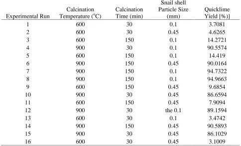
Table 3. Response Factor (Quicklime Yield) for Factorial Analysis of Snail shell Calcination Experimental Design
Experimental Run
Calcination Temperature (P
o
P
C)
Calcination Time (min)
Snail shell Particle Size
(mm)
Quicklime Yield [%)]
1 600 30 0.1 3.7081
2 600 30 0.45 4.6265
3 600 150 0.1 14.2721
4 900 30 0.1 90.5574
5 600 150 0.1 14.419
6 900 150 0.45 90.0164
7 900 150 0.1 94.7322
8 900 150 0.1 94.9663
9 600 150 0.45 9.6854
10 900 30 0.45 86.6594
11 600 150 0.45 7.9094
12 900 30 the 0.1 89.1594
13 600 30 0.1 3.4742
14 900 150 0.45 90.5893
15 900 30 0.45 86.1029
16 600 30 0.45 3.1009
From Table 3, it could be observed that optimum yield of 94.9663 quicklime was obtained at an optimal calcination temperature of 900 P
o
P
C, calcination time of 150 minutes and particle size of 0.1 µm. This revealed that the optimum yield was obtained at higher settings of temperature and time and lower setting of particle size. This could be ascribed to the fact that at a higher temperature of 900 P
o
P
C and time of 150 minutes, there was a complete loss of carbon dioxide and more of quicklime was generated because the lower particle size of 0.1 µm of the samples provided a large surface area for the decomposition of calcium carbonate into quicklime.
3.2 Factorial analysis results showing effects of calcination time and Snail shell particle
size on quicklime yield
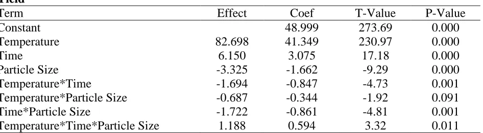
The P-values and the t-distribution were determined to test the statistical significance. The statistics are considered significant when the P-value is less than 0.05 for 95% confidence level. The results of the P-values, coefficients and t-distribution and effects for the quicklime yield are given in Table 3.
Table 4: Factorial Design Analysis for Estimated Effects and Coefficients for Quicklime Yield
Term Effect Coef T-Value P-Value
Constant 48.999 273.69 0.000
Temperature 82.698 41.349 230.97 0.000
Time 6.150 3.075 17.18 0.000
Particle Size -3.325 -1.662 -9.29 0.000
Temperature*Time -1.694 -0.847 -4.73 0.001
Temperature*Particle Size -0.687 -0.344 -1.92 0.091
Time*Particle Size -1.722 -0.861 -4.81 0.001
Temperature*Time*Particle Size 1.188 0.594 3.32 0.011
From the Table, it shows that quicklime yield factorial designs are significant except Temperature*Snail shell Particle Size Interaction. The reason for this exception is that calcination temperature is the pre-requisite and predominant factor required for thermal decomposition of Snail shell to occur and irrespective of the particle size of the snail shell, higher calcination temperature resulted in more yield of quicklime.
Table 4 further revealed some important information regarding the main and interaction effects have on the quicklime yield. The main effects, of temperature, time and Snail shell particle size have effects numbers of 82.698, 6.150, and -3.325, respectively. The magnitude of the effect of temperature is approximately eleven times higher than time twenty times higher than Snail shell particle size because it is the predominant factor required to drive the thermal decomposition reaction to equilibrium. Dogu (2000)[13] reported that calcination temperature is the driving factor for dissociation of Snail shell into CaO and COR2R and the factor required in overcoming the
energy barrier (lowering of the activation energy) required for decomposition of Snail shell to occur. All of the effect numbers are positive except snail shell particle size as an increase in calcination temperature and time results in an increase in quicklime yield. Snail shell particle size is negative as an increase in its value led to a decrease in quicklime yield. Hayes (2014) [14] reported that calcination rate of thermal decomposition of the snail shell is location-dependent and smaller Snail shell particle produced quicklime of higher yield than smaller Snail shell particle. Also, the three main effects are significant statistically at the 95% confidence level. Calcination temperature produced the largest change in quicklime yield compared to all other factors because it has the highest effect number. Thus, increasing the setting of the calcination temperature increased the quicklime yield the most. All two- and three-factor interactions have smaller effect numbers than those of the single-process factors. The results for the factors interaction demonstrate that there is an effect on the quicklime yield when different process factors are combined.
The order of the effects and statistical significance of the formulation can be represented graphically in a Pareto Chart. A Pareto Chart is a bar graph that shows information in order of magnitude to graphically show the relative importance of the differences between groups of data. The Pareto Chart for the quicklime yield is shown in Figure 2.
Fig 2. Pareto Chart of the Standardized Effect for Quicklime Yield
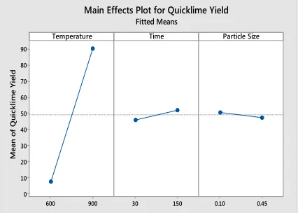
Fig 3. Main Effect Plot for Quicklime Yield
The red line represents the 95% confidence level. If the bar representing a formulation does not cross this line the effect of the quicklime yield is not statistically significant. Again, this graph shows all single and multiple process factors effects are significant for the main effects, Temperature*Time, Temperature*Snail shell Particle Size and Temperature*Time*Snail shell Particle Size at the 95% confidence are significant. Potgieter et al. (2003) [15] has shown that calcination temperature, calcination time and Snail shell particle size play a significant role on thermal decomposition of Snail shell.
3.3 Main effect plot of the fitting means of Figure 4.2 indicates the following:
• Temperature: Calcination temperature produced higher yield at a temperature of 900 P
o
P
C than at a temperature of 600 P
o
P
C as the fitted mean increased from 11 to 94% respectively. This reason can be attributed to COR2R (Loss on Ignition) being continuously released as
Snail shell is thermally decomposed until only CaO is left in the quicklime product. Term
AC ABC AB BC C B A
250 200 150 100 50 0
A Temperature B Time C Particle Size Factor Name
Standardized Effect
2.3
Pareto Chart of the Standardized Effects
(response is Quicklime Yield, α = 0.05)
900 600 90 80 70 60 50 40 30 20 10 0
150
30 0.10 0.45
Temperature
M
ea
n
of
Q
ui
ck
lim
e
Yi
el
d
Time Particle Size
Main Effects Plot for Quicklime Yield
Fitted Means
• Time: Calcination time produced lower yield at low calcination time (30 min) than at high time (150 min) as the fitted mean decreased from the temperature of 48 to 54% respectively. The reason for this is that there is a synergistic effect of time on the quicklime yield as reported by Zhong and Bjerle (1993) [16] due to high residence time in kiln that provided enough time for continuous release of COR2R (Loss on Ignition) as
Snail shell is thermally decomposed until only CaO is left in the quicklime product. Bogwardt, (1985) [17] also supported this observation.
• Snail shell Particle Size: smaller Snail shell particle size (0.1 mm) produced quicklime of higher reactivity than bigger Snail shell particle size (0.45 mm) as the fitted mean decreased from 52 to 48 % respectively. This is in line with the reported observation of Hu and Scaroni (1996) [18]who reported that the calcination rate is location-dependent and smaller Snail shell particles produced quicklime of higher yield than smaller Snail shell particles.
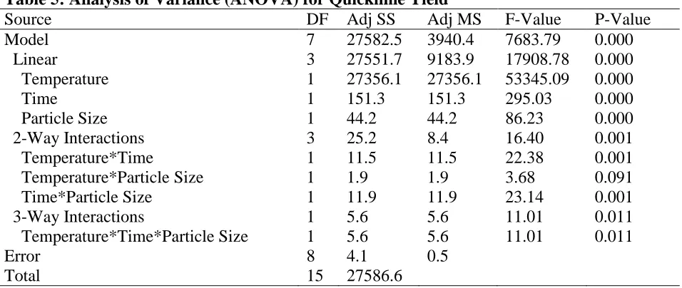
Table 5 shows the ANOVA Table for the quicklime yield. The SS, MS and F-distribution numbers all follow the same order as the rank of effects in the factorial design analysis and the Pareto Chart. According to the P-values reported in the ANOVA Table, all of the process factors were in the 95% confidence level. The ANOVA results support the previously obtained results of coefficient and main effect results of Table 4.
Table 5: Analysis of Variance (ANOVA) for Quicklime Yield
Source DF Adj SS Adj MS F-Value P-Value
Model 7 27582.5 3940.4 7683.79 0.000
Linear 3 27551.7 9183.9 17908.78 0.000
Temperature 1 27356.1 27356.1 53345.09 0.000
Time 1 151.3 151.3 295.03 0.000
Particle Size 1 44.2 44.2 86.23 0.000
2-Way Interactions 3 25.2 8.4 16.40 0.001
Temperature*Time 1 11.5 11.5 22.38 0.001
Temperature*Particle Size 1 1.9 1.9 3.68 0.091
Time*Particle Size 1 11.9 11.9 23.14 0.001
3-Way Interactions 1 5.6 5.6 11.01 0.011
Temperature*Time*Particle Size 1 5.6 5.6 11.01 0.011
Error 8 4.1 0.5
Total 15 27586.6
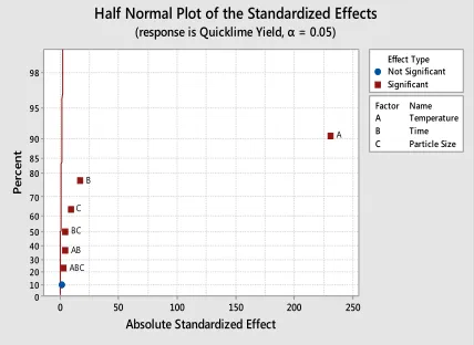
The normal plot of the standardized effect for quicklime yield response of Figure 5 also shows
that there are three significant effects ( = 0.05). Th
main factors calcination temperature (A), calcination time (B) and Snail shell particle size (C). Calcination temperature (A) has the largest effect because it is the furthest from the line. In addition, the Figure also shows the direction of the effect. Calcination temperature (A), calcination time (B) and the combined effects of temperature, time and particle size (ABC) reside to the right of the line and they all have positive effects. This means quicklime yield increases when process variables change from the low to high level. Because Snail shell particle size (C) and the combination of temperature and particle size (AC) resides to the left of the line,
it has a negative effect, meaning that quicklime reactivity decreases when the calcination time and Snail shell particle size change from the low level to the high level.
Fig 5. Normal Plot of the Standardized Effect for Quicklime Yield
Fig 6. Half Normal Plot of the Standardized Effect for Quicklime Yield
For the half-normal probability plot of quicklime yield of Figure 6, there are three significant effects ( = 0.05). All three main factors; calcination temperature (A), calcination time (B), and Snail shell particle size(C) are significant. Calcination temperature (A) has the largest effect because it lies furthest from the line. The half-normal probability plot produces the same rankings as previously discussed for the order of process factors effects and their combination on quicklime yield from Pareto plot, Normal Probability plot and Estimated Effects and Coefficients for quicklime yield.
Since the lines of interaction plot of quicklime yield of Figure 6 are parallel to each other, there may be no interaction present, this due to a synergistic effect between temperature and time on quicklime yield. The plot also shows that a movement of the response means from the low to the high level of calcination temperature is independent of the level of calcination time. The plot indicates that the degree of departure of the two lines of Figure 7 and Figure 8 from being parallel is greater, this infers that the effect is stronger. The plot indicates that the increase in
250 200 150 100 50 0 99 95 90 80 70 60 50 40 30 20 10 5 1 A Temperature B Time C Particle Size Factor Name Standardized Effect Pe rc en t Not Significant Significant Effect Type ABC BC AB C B A Normal Plot of the Standardized Effects
(response is Quicklime Yield, α = 0.05)
250 200 150 100 50 0 98 95 90 85 80 70 60 50 40 30 20 10 0 A Temperature B Time C Particle Size Factor Name
Absolute Standardized Effect
Pe rc en t Not Significant Significant Effect Type ABC BC AB C B A Half Normal Plot of the Standardized Effects
(response is Quicklime Yield, α = 0.05)
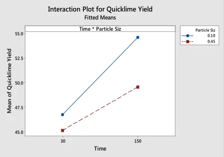
quicklime yield is greater as the calcination time is moved from 30 min to 150 min when the calcination temperature is high (red line) than when it is low (black line). The lines of interaction plot of quicklime yield of Figure 8 are slightly not parallel to each other; there may be the presence of small interaction present. This occurs because of the antagonistic effect between time and Snail shell particle size on quicklime yield. The plot indicates that the increase in quicklime yield is greater as the calcination time is moved from 150 min to 30 min when the calcination temperature is high (red line) than when it is low (black line).
Fig 7. Temperature-Time Interaction Plot for Quicklime Yield
Fig 8. Time-Snail shell Particle Size Interaction Plot for Quicklime Yield
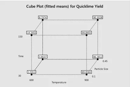
• The cube plot of Figure 9 illustrates that if Snail shell of smaller particle size (0.1 mm) is used, the calcination temperature is high (900 P
o
P
C) and calcination time is high (150 min), the quantity of quicklime yield is 94.8493%. This is corroborated by the work of [16] and [17] that quicklime yield is increased when Snail shell is calcined at high temperature, high residence time and smaller Snail shell particles are used.
900 600
90 80 70 60 50 40 30 20 10 0
Temperature * Time
Temperature
M
ea
n
of
Q
ui
ck
lim
e
Yi
el
d
30 150 Time Interaction Plot for Quicklime Yield
Fitted Means
150 30
55.0
52.5
50.0
47.5
45.0
Time * Particle Siz
Time
M
ea
n
of
Q
ui
ck
lim
e
Yi
el
d
0.10 0.45 Particle Siz Interaction Plot for Quicklime Yield
Fitted Means
Fig 9. Cube Plot for Quicklime Yield
Fig 10. Contour Plot of Quicklime Yield against Time and Temperature
Contour plot of quicklime yield against time and temperature of Figure 10 shows how quicklime yield relates to time and calcination temperature. The darkest green area indicates the contour where the quicklime yield is highest (greater than 80%) while holding Snail shell particle size at 0.1 mm. To maximize quicklime yield, the settings for calcination temperature and calcination time should be chosen.
Figure 11 shows the plot of residuals against fitted values for quicklime yield. The residuals follow a straight line. Also, evidence of skewness, outliers, and non-normality does not exist. This Figure shows the residuals follow the normal probability distribution as all points scatter around a straight line.
0.45
0.1 150
30
900 600
Particle Size Time
Temperature
90.3028
86.3812 3.8637
8.7974
94.8493
89.8584 3.5911
14.3455
Cube Plot (fitted means) for Quicklime Yield
Particle Size 0.275 Hold Values
Temperature
Ti
m
e
900 850 800 750 700 650 600 150
125
100
75
50
> – – – < 20 20 40 40 60 60 80 80 Yield Quicklime
Contour Plot of Quicklime Yield vs Time, Temperature
Fig11. The Normal Probability Plot for Quicklime Yield
Figure 12 shows the plot of residuals against fitted value for quicklime yield. The residuals of Figure 12 are randomly scattered about zero. The plot does not show the presence of outliers, missing terms, and non-constant variance. In other words, the predicted values variation is constant, irrespective of whether their values are small or large.
Fig12. The Plot of Residual against Fitted Value for Quicklime Yield
1.5 1.0
0.5 0.0
-0.5 -1.0
99
95 90
80 70 60 50 40 30 20
10 5
1
Residual
Pe
rc
en
t
Normal Probability Plot (response is Quicklime Yield)
100 80
60 40
20 0
1.0
0.5
0.0
-0.5
-1.0
Fitted Value
R
es
id
ua
l
Versus Fits
(response is Quicklime Yield)
Fig 13. The Plot of Residual against Observation Order for Quicklime Yield
Figure 13 shows the plot of residuals against observation order for quicklime yield. The residuals are randomly scattered about zero. Also, there is no suggestion that the error terms are interrelated to one another. This shows that the residuals scatter randomly.
Based on the normal probability plot, residual against fit plot and the residual against the run order, the estimated regression model is adequate. The model Equation can be built from estimated coefficients for quicklime yield of Table 3
Ypy = 48.999 + 41.349𝑥1+ 3.075𝑥2 − 1.662𝑥3− 0.847𝑥1𝑥2− 0.344𝑥1𝑥3 − 0.861𝑥2𝑥3 +
0.594𝑥1𝑥2𝑥3 (4)
x1: The calcination temperature which has two levels coded 1 and − 1
x2: The calcination time which has two levels coded 1 and − 1
x3: The Snail shell particle size which has two levels coded 1 and − 1
Ypy = Predicted Quicklime yield( %)
Calcination temperature 𝑋1 = � 1, high level
−1, low level
Calcination time𝑋2= � 1, high level
−1, low level
Snail shell particle size𝑋1 = � 1, high level
−1, low level
Based on the Main Effect plot, the combinations of factors that will produce the highest quicklime yield are:
16 15 14 13 12 11 10 9 8 7 6 5 4 3 2 1 1.0
0.5
0.0
-0.5
-1.0
Observation Order
R
es
id
ua
l
Versus Order
(response is Quicklime Yield)
• High level of calcination temperature of 900 P
o
P
C.
• High level of calcination time of 150 min
• Low level of Snail shell particle size of 0.1 mm.
Based on Interaction plot, the combinations of factors that will produce the highest quicklime yield are:
• High level of calcination temperature of 900 P
o
P
C and a high level of calcination time of 150 min.
• High level of calcination temperature 900 P
o
P
C and low level of Snail shell particle size of 0.1 mm.
• High level of calcination temperature of 900 P
o
P
C, high level of calcination time of 150 min and low level of Snail shell particle size of 0.1 mm.
The model Equation via the combination above of main effects and the Interaction plot is:
𝑌 = 48.999 + 41.349(1) + 3.075(1) − 1.662(−1) − 0.847(1)(1) − 0.344(1)(−1) −
0.861(1)(−1) + 0.531(1)(1)(−1) = 94.9663 (5)
Table 6: Statistical Parameters of the Model summary
Statistical Parameters Values
S 0.716111
RP 2 99.99% RP 2 P
adjusted 99.97%
RP
2
P
predicted 99.94%
Table 6 shows the model proportion of the response variability that is (RP
2
P
) is 99.99%, while predicted RP
2
P
the level of prediction of the future data by the model is 99.94%, and the adjusted RP
2
P
useful for comparing models from the same data with different numbers of terms is 99.97%. The RP
2
P
value lies between 0 and 100%. The model predicts better when the RP
2
P
value is closer to 100% [19] The variance (S) for assessing model’s predictive ability from Table 4.4 is 0.716111. Low S value of 0.716111 is an indication that the model fits the data as Montgomery (1999) reported that the model fits the data better when the 0.716111 is smaller. (RP
2
P
) of 99.99%,
adjusted RP
2
P
of 99.97%, predicted RP
2
P
of 99.94% and S value of 0.716111 shows that the model adequately represents the experimental data.
4 Conclusions
This study has demonstrated the application of factorial analysis in determining calcination parameters that are having a significant effect on quicklime yield. From the results of the analysis carried out the following conclusions were obtained.
• From the factorial analyses, the temperature, time and particle size have a significant effect on the quicklime yield.
• The factorial analysis also suggested that there is a significant interaction between calcination temperature and particle size to produce quicklime of high yield.
• Also, optimal quicklime yield of 94.9663%PPwas obtained when quicklime was calcined
with a particle size of 0.1 mm and temperature of 900 P
o
P
C using calcination time of 150 min.
References
[1] N. Marinoni,., S. Allevi., M. Marchi., & M. Dapiaagi. “A Kinetic Study of Thermal Decomposition of Limestone Using In Situ High-Temperature X-Ray Powder Diffraction”. Journal of American Ceramic Society, 95 (8), (2012), 2491-2498.
[2] S. Yusuf. “Kinetics Study of Calcination of Ashaka Limestone Using Coats-Redfern Method”. MEng Thesis, Chemical Engineering Department, Federal University of Technology, Minna, Nigeria. (2015)
[3] A. Moropoulou., A. Bakolas., & E. Aggelakopoulou. “The Effect of Snailshell Characteristics and Calcination Temperature to the Reactivity of Quicklime”. Cement
and Concrete Research, 31, (2001), 633-639.
[4] N. M. Bello. “Calcination Kinetics of Okpella Limestone from Thermogravimetric Data for Limes Production” MEng Thesis, Chemical Engineering Department, Federal University of Technology, Minna, Nigeria. (2015)
[5] H. F. Akande, “Multiple Response Optimization of Quicklime Production from Limestone Using Design of Experiment”. Minna: Ph.D. Thesis, Chemical Engineering Department Federal University of Technology, Minna, Nigeria. (2015)
[6] J. H. Oates. Lime and Limestone: Chemistry and Technology, Production and Uses. Weinheim: Wiley-VCH, (1998).
[7] M. Hassibi. “An Overview Of Lime Slaking And Factors That Affect The Process”. Washington D.C.: Chemco Systems, L.P. (1999).
[8] Z. Kilic & M. Anil. “Effects of Snailshell Characteristic Properties and Calcination Temperature on Lime Quality”. Asian Journal of Chemistry 18. (2006). 655-666
[9] A. Khodaii., H. F. Haghshenas & H. K. Tehrani. “Effect of grading and lime content on HMA stripping using statistical methodology” Construction and Building Materials 34, (2012),131–135.
[10] D. C. Montgomery “Design and Analysis of Experiments”. New York: John Wiley & Sons. (2005).
[11] D. B. Soares., E. C. Hori & E. A. Batista. “Optimization of the Production Quicklime by Calcination in Rotary Kilns”.Material Science Forum Vols. (2008), 591-593.
[12] A. Meier., E. Bonaldi., G. Cella., W. Lipinski., D. Wuillemin., & R. Palumbo. “Design and Experimental Investigation of a Horizontal Rotary Reactor for The Solar Thermal Production Of Lime”. Energy, 29, (2004), 811-821.
[13] G. Dogu, & A. Irfan “Calcination Kinetics of High Purity Limestones”. Chemical
Engineering Journal, (2001). 1-2.
[14] F. O. Hayes “Optimization Studies of Quicklime Production From Obajana Snailshell Using One Variable at A Time Method”. HND Thesis, Department of Chemical Engineering, Kaduna Polytechnic, Kaduna, Nigeria.
[15] J. H. Potgieter., S.S Potgieter & D. De Waal “An empirical study of factors Influence lime slaking: Part II. Influence of Material and water composition”. Water SA 29 (2) (2003), 157-160.
[16] 22T Q15T22T.0T15T Zhong 0T15T&0T15T0T22TI15T22T.0T15T Bjerle “0TCalcination Kinetics of Limestone and the Microstructure of
Nascent CaO”. 47TThermochimica Acta0T47T0T58T223,0T58T (1993), 0T46T109-120.
[17] R. H. Borgwardt “Calcination Kinetics and Surface Area of Dispersed Limestone Particles”. AIChE Journal, 31 (1), (1985), 103-111.
[18] N. Hu., & A.W. Scaroni “Calcination of Pulverized Limestone Particles under Furnace Injection Conditions”. Fuel, 75, (1996), 177-186.
[19] 18TK.K. Doddapaneni., R. Tatineni., R. Potumarthi., L. N. Mangamoori “Optimization of
media constituents through response surface methodology for the improved production of alkaline proteases by 18T20TSerratia rubidaea”18T20T. 18T51TJ Chem Technol Biotechnology.18T51T;18T52T8218T52T: (2007),
721–729.