1
Robust Constrained Model Predictive Control
Based on Parameter-Dependent Lyapunov
Functions
Yuanqing Xia1, G. P. Liu2, P. Shi2, J. Chen1, D. Rees2
1Department of Automatic Control
Beijing Institute of Technology Beijing, 100081, China
xia [email protected];[email protected]
2Faculty of Advanced Technology
University of Glamorgan Pontypridd, CF37 1DL, United Kingdom [email protected];[email protected];[email protected]
Abstract: The problem of robust constrained model predictive control (MPC) of systems with polytopic uncertainty is considered in this paper. New sufficient conditions for the existence of parameter-dependent Lyapunov functions are proposed in terms of linear matrix inequalities (LMIs), which will reduce the conservativeness resulting from using a single Lya-punov function. At each sampling instant, the corresponding parameter-dependent LyaLya-punov function is an upper bound for a worst-case objective function, which can be minimized using the LMI convex optimization approach. Based on the solution of optimization at each sampling instant, the corresponding state feedback controller is designed, which can guar-antee that the resulting closed-loop system is robustly asymptotically stable. In addition, the feedback controller will meet the specifications for systems with input or output constraints, for all admissible time-varying parameter uncertainties. Numerical examples are presented to demonstrate the effectiveness of the proposed techniques.
I. INTRODUCTION
MPC, also known as Receding horizon control (RHC), is an on-line technique in which the current control action is computed at each time step by solving a finite horizon open-loop optimal control problem that extends from the current time to the current time plus a specified horizon length. The current state of the plant is used as the initial state, and the first control in the sequence obtained by optimization is applied to the plant. A full review of the recent advances related to MPC can be found in a survey paper [1]. In practice, there are always modelling errors, and it is necessary to consider robust MPC in the presence of model uncertainty. Recently, many research results in the design of robust MPC have appeared, see for example, [2], [3], [4], [5], [6] and the reference therein. On the other hand, the main drawback associated to the above mentioned methods proposed in MPC is that a single Lypunov matrix is used to guarantee the desired closed-loop multiobjective specifications. This must work for all matrices in the uncertain domain to ensure that the hard constraints on inputs and outputs are satisfied. This condition is generally conservative if used in time-invariant systems. Furthermore, the hard constraints on outputs of closed-loop systems can not be transformed into an LMI form using the method proposed in [2], [3], [5].
II. PROBLEM STATEMENT
We consider the following class of uncertain discrete-time systems
x(k+ 1) =A(k)x(k) +B(k)u(k)
y(k) =C(k)x(k) (1)
where x(k) ∈ Rn is the state, u(k) ∈ Rl is the control input, y(k) ∈ Rm is the plant output,
A(k), B(k), C(k)are uncertain matrices which are assumed to belong to a polytopic convex domain:
A(k) B(k)
C(k) 0
∈Ω (2)
For polytopic uncertainty,Ωis the polytope Co{
A1 B1
C1 0
,· · ·,
Ap Bp
Cp 0
}, whereCodenotes
the convex hull,
Ai Bi
Ci 0
are vertices of the convex hull. Any
A(k) B(k)
C(k) 0
within the convex
set Ω is a linear combination of the vertices
A(k) B(k)
C(k) 0
=
p
X
i=1
ξi(k)
Ai Bi
Ci 0
(3)
where Ppi=1ξi(k) = 1, ξi(k)≥0.
Remark 1: Note that relation (2) defines a polyhedral type of uncertainty domain. In fact, the important case of interval matrices can exactly be modelled by this kind of uncertainty with appropriate choice of the extreme matrices. Being convex and polyhedral, this kind of uncertainty is clearly more general than interval matrix domains. The design of MPC with polytopic uncertainty is considered in [2], [3], [5], [6], and the matrix C was assumed to be constant in [2], [3]. In (3), the parameters are time-varying in a certain range during operation. Then, the uncertain discrete-time system (1) is time-varying. So the robust stability conditions for system (1) will be more strict than the case that unknown parameter are constant [10].
Consider the following problem, which minimizes the worst case quadratic objective function in an infinite horizon:
min
J∞= ∞
X
i=0
[x(k+i|k)TQ0(k+i|k) +u(k+i|k)TR0u(k+i|k) (5) whereQ0 >0 andR0 >0 are known weighting matrices,F(k) is the feedback matrix gain obtained at sampling instant k, which will be denoted as F for simplicity. The optimal problem (4) is subject to (1) and
|uh(k+i|k)| ≤uh,max, i≥0, h= 1,2,· · ·, l (6)
|yh(k+i|k| ≤yh,max, i≥1, h= 1,2,· · ·, m (7)
x(k+i|k) andy(k+i|k) are the state and output respectively, at timek+i, predicted based on the measurements at timek;x(k|k)andy(k|k) refer respectively to the state and output measured at time
k;u(k+i|k) is the control move at timek+i, computed by the optimization problem (4) at time k;
u(k|k) is the control move to be implemented at time k.
Remark 2: In the control theory, especially control engineering, control problems where variables need to satisfy constraints and where the control action also has to minimize a cost arise naturally and received much consideration. One effective control algorithm that addresses such problems is model predictive control (MPC), this method proposes a framework to deal with constrained control problems for which the classical off-line computation of control laws is rendered difficult or impossible. Due to the merit of this method, MPC has become a widely used technique to address advanced control problems in industrial applications, such as chemical process control [11].
III. MAINRESULTS
To begin this section, we first recall the following lemmas which will be used in the proof of our main results.
Lemma 1: ([12]) The following conditions are equivalent:
i There exists a symmetric matrix P >0 such that
ATP A−P <0 (8)
ii There exist a symmetric matrixP and a matrix G such that
P ATG
GTA G+GT −P
>0 (9)
i There exists a symmetric positive definite matrix P such that
x(k|k)TP x(k|k)< γ (10)
ii There exist a symmetric positive definite matrix P and a matrix V such that
−γ x(k|k)T
x(k|k) P−V −VT
<0 (11)
Proof: Firstly, we will prove that (10) is equivalent to the existence of matrix G and positive definite matrix P˜ such that
−γ x(k|k)TG
GTx(k|k) P˜−GT −G
<0 (12)
Sufficiency: Since the matrix h 1 x(k|k)T
i
has full rank, (12) implies that
h
1 x(k|k)T i
−γ x(k|k)TG
GTx(k|k) P˜−GT −G
1
x(k|k)
<0 (13)
letting P˜ =P, which leads to (10).
Necessity: Assuming (10) is satisfied, and using Schur complement, (10) is equivalent to
−γ x(k|k)TP
PTx(k|k) −P
<0 (14)
Then choosing G=GT =P = ˜P, the above inequality can be written as
−γ x(k|k)TG
GTx(k|k) P˜−G−GT
<0 (15)
Secondly, it will be shown that (12) is equivalent to the existence of matrix G and a symmetric
positive definite matrix P such that (11) holds. Pre-and post-multiplying (12) by
1 0
0 G−T
and
1 0
0 G−1
on both sides, and letting V =G−1 and P =G−TP G˜ −1, we obtain (11).
As quadratic objective J∞ defined (5) is difficult to be obtained. An possible way is to find an
upper bound onJ∞, then we can design the controller such that the upper bound is minimized respect
V(x(k|k)) =x(k|k)TP(ξ(k))x(k|k), is defined at sampling time k, where P(ξ(k)) is a
parameter-dependent positive definite matrix. For any [A(k+i) B(k+i)]∈Ω, i >0, suppose that V(x(k|k)) satisfies the following robust stability constraint:
V(x(k+i+ 1|k))−V(x(k+i|k))≤ −[x(k+i|k)TQ0x(k+i|k) +u(k+i|k)TR0u(k+i|k)] (16) As it is assumed that the summation is up to ∞, i.e.,i→ ∞, x(i|k) should approach zero, that is,
x(∞|k) = 0. Summing (16) fromi= 0 to∞ leads to the following inequality
max
[A(k+i) B(k+i)]∈Ω,i>0J∞(k)≤V(x(k|k)) (17) From the above inequality, it shows thatV(x(k|k))is just an upper bound onJ∞, thus in the following
theorem, the controller is designed such thatV(x(k|k)) is minimized at sampling timek.
In [13] and [10], the method of parameter-dependent Lyapunov function has been adopted. Es-pecially, in [10] the results have been improved further compared to the results in [13]. But, the it can not be proved that the resulting closed-loop system is robustly stable based on the algorithm proposed in [13] and [10], which was neglected in paper [13] and [10]. Firstly, at sampling k, the control feedback is designed such that the upper bound on V(x(k|k)) is minimized, which is little different to Theorem 1 in [13] and Theorem 2 in [10].
Theorem 1: Letx(k) =x(k|k)be the state of the uncertain system (1) measured at sampling time
k. If the convex optimization problem for
min
E,Pj,V
γ (18)
subject to
−γ x(k|k)T
x(k|k) Pj(k)−V −VT
<0 (19)
−Pi(k) VTATj +ET(k)BjT ET(k)R0 VTQ0
AjV +BjE(k) Pj(k)−V −VT 0 0
E(k)R0 0 −R0 0
V Q0 0 0 −Q0
<0
∀j= 1,2,· · ·, p and i= 1,2,· · ·, p
(20)
has a solution in the matrix variablesPj(k)>0, j = 1,2,· · ·, p,E(k),V andγ, then, the
parameter-dependent Lyapunov function can be taken as
where P(i, k) =Ppj=1ξj(i+k)Pj(k)and a state feedback control gain matrix F(k) =E(k)V−1 in
the control law can be chosen as u(k+i|k) =F(k)x(k+i|k), i≥0 such that the upper bound of
V(x(k|k)) := x(k|k)TP(ξ(k))x(k|k)
:= x(k|k)TV−TP(0, k)V−1x(k|k) := x(k|k)TV−T Pp
j=1ξj(k)Pj(k)V−1x(k|k)
:= x(k|k)TV−TP(ξ(k))V−1x(k|k)
(22)
on the robust performance objective function is minimized at sampling time k.
Proof. The derivation of formula (20) is very similar to that in [10], which is omitted here.
Note that minimization of V(k|k) =x(k|k)TP(ξ(k))x(k|k) is equivalent to
min
γ,P(ξ(k))γ (23) subject to
x(k|k)TP(ξ(k))x(k|k)< γ (24) It follows from Lemma 2 that (24) is equivalent to the existence of matricesP(ξ(k))andV such that
−γ x(k|k)T
x(k|k) P(ξ(k))−V −VT
<0 (25)
For each j, multiply (19) corresponding j= 1,2,· · ·, p inequalities byξi(k)≥0 and sum, then, it is
shown that (25) is satisfied if (19) holds. Thus, the proof is completed.
Remark 3: The Lyapunov function, V(x(k|k)) = x(k|k)TV−TP(ξ(k))V−1x(k|k), adopted in Theorem 1 is parameter-dependent. It is different from the result in Theorem 1 in [2], in which a single Lyapunov matrix V−TP(ξ(k))V−1 = P, i.e., Lyapunov function V(x(k|k)) = x(k|k)TP x(k|k) is
used, that is, the inequalities (18)-(20) are required to be satisfied with a fixedP for all[A(k)B(k)]∈
Ω, which is also called quadratic stability and has many successful applications in robust control theory and filtering design although it brings conservativeness in some sense. This concept has been extensively used in many papers, such as [14], [15] and the references therein. More recently, the problem of MPC with parameter-dependent Lyapunov function has been considered in [13] and [10], but the uncertainties does not exit in all system matrix, while it is very natural that all the systems are subjected to time-varying uncertainties.
Theorem 2: The feasible receding horizon state feedback control obtained by optimization at each sampling instant in Theorem 1, i.e., (u(0|0), u(1|1),· · ·, u(k|k), k → ∞), robustly asymptotically stabilizes the resulting closed-loop system (1).
Proof:: See the proof in the Appendix.
When there are constraint bounds on the inputu(k+i|k) and output y(k+i|k), a similar idea to [2] can be used to transform the constraints into LMI forms, which leads to the following result.
Theorem 3: Letx(k) =x(k|k)be the state of the uncertain system (1) measured at sampling time
k. If the convex optimization problem
min
E,Pˆj,Qj,V
γ (26)
subject to
−1 x(k|k)T
x(k|k) Pˆj−V −VT
<0 (27)
subject to
−Pˆi VTAT
j +ETBjT ETR0 VTQ0
AjV +BjE Pˆj−V −VT 0 0
ER0 0 −γR0 0
V Q0 0 0 −γQ0
<0
∀j= 1,2,· · ·, p and i= 1,2,· · ·, p
(28)
−Z E
ET −Pˆj
<0,with Z(hh)< u2
h,max, h= 1,2,· · ·, r (29)
−Uj (AjV +BjE)
(AjV +BjE)T −Pˆj
<0 (30)
−S CjHT
HCT
j Uj−H−HT
<0,with S(hh)< y2
h,max, h= 1,2,· · ·, m (31)
has a solution in the matrix variables Pˆj > 0, Qj > 0, j = 1,2,· · ·, p, E, H and V. Then, the
parameter-dependent Lyapunov function can be taken asV(x(k|k)) =x(k|k)TV−TPp
j=1ξjPˆjV−1x(k|k)
i the feasible receding horizon state feedback control law u(k|k) = F x(k|k), k ≥ 0, i.e., (u(0|0), u(1|1),· · ·, u(k|k), k→ ∞), obtained by the optimization at each sampling instant robustly asymptotically stabilizes the resulting closed-loop system (1);
ii the upper bound ofV(x(k|k))on the robust performance objective function is minimized at sampling time k;
iii the component-wise peak bound on uh(k+i|k) satisfies
uh(k+i|k)| ≤uh,max, i≥0, h= 1,2,· · ·, l; (32)
iv the component-wise peak bound on yh(k+i|k) satisfies
yh(k+i|k)| ≤yh,max, i≥0, h= 1,2,· · ·, m. (33)
Proof: Assume that the inequalities of (28) are satisfied, it can be easily shown that (20) are also satisfied with Pˆ replaced by 1
γP. Then using the same as that in Theorem 1, it can be proved that
(16) are satisfied for i≥ 0. Thus, it follows from (16) and (17) that the following inequalities hold for all i≥0
V(x(k+i+ 1|k))≤V(x(k+i|k))≤V(x(k|k))≤γ (34)
Let Pˆj = γ1Pj andP˜(ξ(k)) = 1γP(ξ(k)). Then
˜
P(ξ(k)) = 1
γV
−T p
X
j=1
ξj(k)Pj(k)V−1 =V−T p
X
j=1
ξj(k) ˆPj(k)V−1
The above inequality implies
x(k+i+ 1|k)TP˜(ξ(k))x(k+i+ 1|k)≤x(k+i|k)TP˜(ξ(k))x(k+i|k)T
≤x(k|k)TP˜(ξ(k))x(k|k)≤1 (35) So the peak bounds on each component ofu(k+i|k) at sampling time k can be expressed as
max
i≥0 |uh(k+i|k)|
2 = max
i≥0 |(EV
−1x(k+i|k))
h|2
≤max
i≥0 |(EP
1 2(ξ) ˆP−
1
2(ξ)V−1x(k+i|k))))h|2
≤( ˆP−12(ξ)ETEPˆ− 1
2(ξ))hhkxT(k+i|k)V−TPˆ(ξ(k))V−1x(k+i|k)k
= ( ˆP−12(ξ)ETEPˆ− 1
2(ξ))hhxT(k+i|k) ˜P(ξ(k))x(k+i|k)
From inequality (35), we have
max
i≥0 |uh(k+i|k)|
2 ≤(( ˆP−1
2(ξ)ETEPˆ− 1
It follows from the above inequalities and matrix theory that (32) hold if the following inequalities are satisfied:
−Z E
ET −Pˆj
<0,with Z(hh)< u2
h,max, h= 1,2,· · ·, l (37)
The rest of the proof is similar to that of Theorem 1 with Pˆj = 1γPj, for j= 1,2,· · ·, p.
In order to prove that (33) is satisfied, we only need to show that if (30) and (31) are satisfied, then the constraints on (33) hold for all i≥0, j = 1,2,· · ·, m. With the feedback control law obtained at sampling time k, we have
max
i≥0 |yh(k+i|k)|
2 = max
i≥0 |C(A(k+i) +B(k+i)F)x(k+i|k))h| 2
≤max
i≥0 |(C(A(k+i) +B(k+i)F)V ˆ
P−12(ξ) ˆP 1
2(ξ)V−1x(k+i|k))))h|2
≤ |(C(A(k+i) +B(k+i)EV−1)VPˆ−12(ξ))j|2×
kxT(k+i|k)V−TPˆ(ξ(k))V−1x(k+i|k)k
Note that xT(k+i|k)V−TPˆ(ξ(k))V−1x(k+i|k) = xT(k+i|k) ˜P(ξ(k))x(k+i|k) and (35) hold,
then
max
i≥0 |yh(k+i|k)|
2 ≤( ˆP−1
2(ξ)(A(k+i)V +B(k+i)E)TCTC(A(k+i)V +B(k+i)E) ˆP− 1 2(ξ))hh
Based on the above inequalities and the matrix theory, inequalities (7) hold if the following inequalities are satisfied for all ξ(k+i)∈Ω:
−S C(AjV +BjE)
(C(AjV +BjE))T −Pˆj
<0,with Shh< y2
h,max, h= 1,2,· · ·, m (38)
It follows from (38) that
C(AjV +BjE) ˆPj−1(AjV +BhE)TCT < S
The above inequalities hold if there exist positive definite matricesUj such that the following inequal-ities are satisfied for j= 1,2,· · ·, p
Uj >(AjV +BjE) ˆPj−1(AjV +BjE)T (39)
Using Schur complement and Lemma 1, inequalities (39) and (40) are equivalent to the following inequalities
−Uj (AjV +BjE)
(AjV +BjE)T −Pˆj
<0 (41)
and
−S CjHT
HCT
j Uj−H−HT
<0 (42)
where H is an extra matrix variable. The rest of the proof is similar to that of Theorem 1, thus the proof is completed.
Remark 4: Note that in [2], it is assumed that the matrix C is known and constant, otherwise, the LMI condition of the constraints on outputs can not be obtained using the method proposed in [2]. In system (1), besides A and B, C can also be an uncertain matrix, and the constraints on outputs can be easily transformed into LMIs by the method proposed in this paper. Hence, the results obtained have covered those in [2] as a special case. It should be pointed out that the algorithm is easy to be implemented. The control in put u(k|k) is obtained at sampling time k by convex optimization in Theorem 1. If there are additional constraints on input and outputs, the control input u(k|k) can be obtained at sampling time k by convex optimization in Theorem 3.
IV. EXAMPLE
In this section, one example will be provided to illustrate the effectiveness of the techniques developed in this paper. As the method proposed in [2] is a special case of our methodology, the optimization problem should be feasible using the method proposed in this paper since it is solvable using the approach in [2]. However, the optimization may not have a solution by the result in [2], while it has a solution by our result.
system (1) with
A1 =
−0.90 0.80
0.35 0.45
, A2 =
0.90 0.85
0.40 −0.85
, A3 =
0.96 0.13
0.28 −0.90
B1 =
1
−1
, B2 =
1
−0.8
, B3 =
1
−0.86
(43)
C1=
h
1 0.3
i
, C2 =
h
0.8 0.2
i
, C3=
h
1.2 0.4
i
,
It is shown that the optimization is unfeasible with the method proposed in [2] without these con-straints. However, taking output constraints withy1,max= 2 and input constraints withu1,max= 0.8,
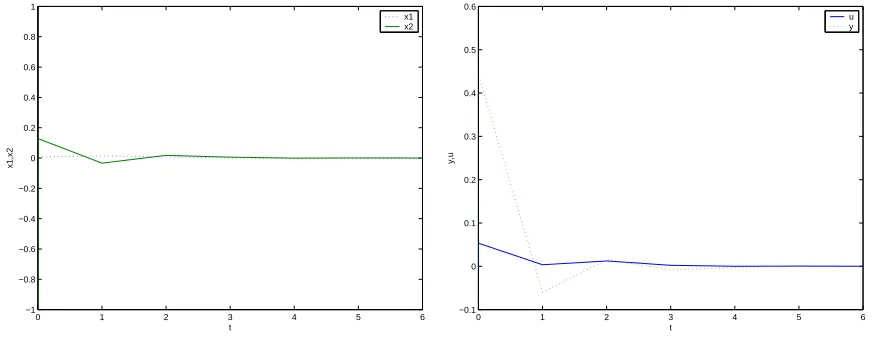
and uncertain parameters are assumed to beξ1(k) = 0.5cos(k)cos(k), ξ2(k) = 0.6sin(k)sin(k), ξ3(k) = 0.5cos(k)cos(k) + 0.4sin(k)sin(k), it is feasible using the method proposed in this paper. The simulation results are given in Fig. 1:
0 1 2 3 4 5 6
−1 −0.8 −0.6 −0.4 −0.2 0 0.2 0.4 0.6 0.8 1 t x1,x2 x1 x2
0 1 2 3 4 5 6
−0.1 0 0.1 0.2 0.3 0.4 0.5 0.6 t y,u u y
Fig. 1: States (x1,x2), output y and input u (method in this paper)
From the simulation with LMI-toolbox in Matlab, it is very effective to design the controller based on the method proposed in this paper. However, it should be mentioned that the complexity of computation will grow quickly with the increase of vertices of the convex set. Due to development of computer techniques, the difficulties can be overcomed.
The problem of robust constrained model predictive control based on parameter-dependent Lya-punov functions with polytopic type uncertainty has been addressed in this paper. The results are based on a new extended LMI characterization of the quadratic objective, hard constraints on inputs and outputs. Sufficient conditions in LMI do not involve the product of the Lyapunov matrices and the system dynamic matrices. The state feedback control guarantees the closed-loop system is robustly stable and the hard constraints on inputs and outputs are satisfied. The approach developed here provides a way to reduce the conservativeness of the existing conditions by decoupling the control parameterization from the Lyapunov matrix.
ACKNOWLEDGMENT
The authors would like to thank the reviewers for their very helpful comments and suggestions which have improved the presentation of the paper. The work of Yuanqing Xia was supported by the National Natural Science Foundation of China under Grant 60504020 and Excellent young scholars Research Fund of Beijing Institute of Technology 2006y0103, respectively. Peng Shi would like to acknowledge the support from Harbin Institute of Technology; Nanjing University of Aeronautics and Astronautics; and LCSIS, Institute of Automation, Chinese Academy of Sciences.
REFERENCES
[1] D. Q. Mayne, J. B. Rawlings, C. V. Rao, and P. O. M. Scokaert, “Constrained model predictive control: stability and optimality,”Automatica, vol. 36, pp. 789–814, 2000.
[2] M. V. Kothare, V. Balakrishnan, and M. Morari, “Robust constrained model predictive control using linear matrix inequalities,”Automatica, vol. 32, pp. 1361–1379, 1996.
[3] Z. Wan and M. V. Kothare, “An efficient off-line formulation of robust model predictive control using linear matrix inequalities,”Automatica, vol. 39, pp. 837–846, 2003.
[4] B. Pluymers, J. A. K. Suykens, and B. D. Moor, “Min-max feedback mpc using a time-varying terminal constraint set and comments on “efficient robust constrained model predictive control with a time-varying terminal constraint set,”
Systems & Control Letters, vol. 54, pp. 1143–1148, 2005.
[5] Y. I. Lee, M. Cannon, and B. Kouvaritakis, “Extended invariance and its use in model predictive control,”Automatica, vol. 41, pp. 2163–2169, 2005.
[6] S. C. Jeong and P. Park, “Constrained mpc algorithm for uncertain time-varying systems with state-delay,” IEEE Transactions on Automatic Control, vol. 50, no. 2, pp. 257–263, 2005.
[8] M. C. de Oliveira, J. Bernussou, and J. C. Geromel, “A new discrete-time robust stability condition,”Systems & Control Letters, vol. 37, pp. 261–265, 1999.
[9] J. C. Geromel, M. C. de Oliveira, and J. Bernussou, “Robust filtering of discrete-time linear systems with parameter dependent lyapunove functions,”SIAM Journal on Control and Optimization, vol. 41, pp. 700–711, 2002.
[10] W. J. Mao, “Robust stabilization of uncertain time-varying discrete systems and comments on ”an improved approach for constrained robust model predictive control”,”Automatica, vol. 39, pp. 1109–1112, 2003.
[11] T. Perezn and H. Haimovich and G. C. Goodwin, “On optimal control of constrained linear systems with imperfect state information and stochastic disturbances”,”International Journal of Robust and nonlinear Control, vol. 14, pp. 379–393, 2004.
[12] M. C. de Olivera, J. C. Geromel, and J. Bernussou, “An LMI optimization approach to multiobjective controller design for discrete-time systems,” inPro. 38th Conf. Decision and Control, (USA), pp. 3611–3616, 1999.
[13] F. Cuzzola, J. Jeromel, and M. Morari, “An improved approach for contrained robust model predictive control,”
Automatica, vol. 38, pp. 1183–1189, 2002.
[14] P. P. Khargonekar, I. R. Petersen, and K. Zhou, “Robust stabilization of uncertain linear systems: quadratic stabilization andH∞ control theory,”IEEE Transactions on Automatic Control, vol. 35, pp. 356–361, 1990.
[15] L. Xie and Y. C. Soh, “Positive real control problem for uncertain linear time-invariant systems,”Systems and Control letters, vol. 24, pp. 265–271, 1995.
[16] M. C. de Oliveira and J. C. Geromel, “A class of robust stability conditions where linear parameter dependence of the lyapunov function is a necessary condition for arbitrary parameter dependence,”Systems & Control Letters, vol. 54, pp. 1131–1134, 2005.
APPENDIX
Proof of Theorem 2: In order to show that the closed-loop system (1) is robustly asymptotically stable, we need to provex(k|k)→0, as k→0. Thus, in the following, we will prove the parameter-dependent Lyapunov function
V(x(k|k)) =x(k|k)TP(ξ(k))x(k|k) =x(k|k)TV−T
p
X
j=1
ξj(k)Pj(k)V−1x(k|k) (44)
k= 1,2,· · ·,∞, obtained at each sampling instant is a strictly decreasing function.
First, we will show:V(x(k+ 1|k+ 1)with the convex minimal Lypunov matrix solutionP(ξ(k)) obtained at samplingkmust be less thanV(x(k|k)with the convex minimal Lypunov matrix solution
P(ξ(k)) obtained at sampling time k, that is,
At sampling time k, taking the parameter-dependent Lyapunov function as
V(x(k|k)) =x(k|k)TV−T
p
X
j=1
ξjPj(k)V−1x(k|k) =x(k|k)TP(ξ(k))x(k|k) (46) which is defined in Theorem 1. From Theorem 1, an upper bound of V(x(k|k)) is minimized at sampling time k with optimal solution (γ(k), Pj(k), j = 1,2,· · ·, p, E(k), V). Then (18)-(20) in
Theorem 1 are satisfied with this optimal solution. When i = j, multiplying inequality (20 ) in Theorem 1 with ξl, for l= 1,2,· · ·, p for eachj, which leads to
−P(ξ(k)) VTA(k)T +ET(k)B(k)T ET(k)R
0 VTQ0
A(k)V +B(k)E P(ξ(k))−V −VT 0 0
E(k)R0 0 −R0 0
V Q0 0 0 −Q0
<0 (47)
Note that the following inequality always holds:
VTP(ξ(k))−1V −V −VT +P(ξ(k)) = (VTP(ξ(k))−1−I)P(ξ(k))(VTP(ξ(k))−1−I)T ≥0 (48)
which means that
P(ξ(k))−V −VT ≥ −VTP(ξ(k))−1V
then, it follows from (47) that
−P(ξ(k)) VTA(k)T +ET(k)B(k)T ET(k)R0 VTQ0
A(k)V +B(k)E −VTP(ξ(k))−1V 0 0
E(k)R0 0 −R0 0
V Q0 0 0 −Q0
<0 (49)
Note thatE(k) =F(k)V, then, by Schur complement, (49) is equivalent to the following inequality:
(A(k) +B(k)F(k))TP(ξ(k))(A(k) +B(k)F(k))−P(ξ(k))< FTR0F +Q0 (50) Pre- and post-multiplying the above inequality byx(k|k)T andx(k|k)on both sides, respectively, we have
x(k|k)T((A(k) +B(k)F(k))TP(ξ(k))(A(k) +B(k)F(k)))x(k|k)
for x(k|k) 6= 0. Note that x(k+ 1|k+ 1) = [A(k) +B(k)F]x(k|k) for [A(k) B(k)] ∈ Ω, where
x(k+ 1|k+ 1) means the state measured atk+ 1, then it follows from the above inequality that the following inequality holds for x(k|k)6= 0
x(k+ 1|k+ 1)TP(ξ(k))x(k+ 1|k+ 1)−x(k|k)TP(ξ(k))x(k|k)< x(k|k)T(FTR0F+Q0)x(k|k) which leads to
x(k+ 1|k+ 1)TP(ξ(k))x(k+ 1|k+ 1)< x(k|k)TP(ξ(k))x(k|k) (51) Next, we will prove that the optimal solution (γ(k), Pj(k), j = 1,2,· · ·, p, V, E(k)) obtained by
optimization at sampling time k is also a feasible solution to that at the sampling time k+ 1, that is, we should prove (γ(k), Pj(k), j = 1,2,· · ·, p, V, E(k))satisfies the following inequalities:
−γ x(k+ 1|k+ 1)T
x(k+ 1|k+ 1) Pj(k)−V −VT
<0 (52)
−Pi(k) VTATj +ET(k)BjT ET(k)R0 VTQ0
AjV +BjE(k) Pj(k)−V −VT 0 0
E(k)R0 0 −R0 0
V Q0 0 0 −Q0
<0
∀j= 1,2,· · ·, p andi= 1,2,· · ·, p.
(53)
Obviously, (γ(k), Pj(k), j = 1,2,· · ·, p, V, E(k)) satisfies (53) since it is the same as the one at
sampling time k. Then we only need to show that (γ(k), Pj(k), j = 1,2,· · ·, p, V, E(k)) satisfies
(52).
It follows from (53) by Schur complement that
−Pi(k) +ET(k)R0E+VTQ0V VTATj +ET(k)BjT
AjV +BjE(k) Pj(k)−V −VT
<0 (54)
which implies
−Pi(k) VTAjT +ET(k)BjT
AjV +BjE(k) Pj −V −VT
<0 (55)
For each i, multiply the above corresponding j = 1,2,· · ·, p inequalities by σi(k) ≥ 0 and sum.
Multiply the resulting i = 1,2,· · ·, p inequalities by ξ(k) ≥ 0 and sum. Taking into account
Pp
j=1σj(k) = 1 andPpi=1ξi(k) = 1, results in
−P˜(σ(k)) VTAT(k) +ETBT(k)
A(k)V +B(k)E P(ξ(k))−V −VT
whereP˜(σ(k)) =Ppi=1σi(k)Pi(k). Pre- and post-multiplying (56) by
V−T 0
0 I
and
V−1 0
0 I
on both sides, and from F(k) =E(k)V−1, we obtain
−V−TP˜(σ(k))V−1 (A(k) +B(k)F)T
(A(k) +B(k)F) P(ξ(k))−V −VT
<0 (57)
By Schur complement, (57) implies
(A(k) +B(k)F(k))T(V +VT −P(ξ(k)))−1(A(k) +B(k)F)< V−TP˜(σ(k))V−1 (58) It follows from (48) that the following inequality always holds:
V−TP˜(σ(k))V−1≤(V +VT −P˜(σ(k)))−1 (59) Comparing (59) with (58), we have
(A(k) +B(k)F)T(V +VT −P(ξ(k)))−1(A(k) +B(k)F)<(V +VT −P˜(σ(k)))−1
Pre- and post-multiplying both sides of the above inequality with x(k|k)T andx(k|k), respectively,
and noting that x(k+ 1|k+ 1) = (A(k) +B(k)F)x(k|k), we have
x(k+ 1|k+ 1)T(V +VT −P(ξ(k)))−1x(k+ 1|k+ 1)< x(k|k)(V +VT −P˜(σ(k)))−1x(k|k) (60) Since (γ(k), Pj(k), j= 1,2,· · ·, p, E(k), V) is the optimal solution obtained at sampling k, it satisfies
−γ(k) x(k|k)T
x(k|k) Pj(k)−VT −V
<0, j= 1,2,· · ·, p
By the convex combination with σi(k), it follows from the above inequalities that
−γ(k) x(k|k)T
x(k|k) P˜(σ(k))−VT −V
<0
By Schur implement, the above inequality is equivalent to
x(k|k)T(V +VT −P˜(σ(k))−1x(k|k)< γ (61) Comparing (61) with (60), we have
x(k+ 1|k+ 1)T(V +VT −P(ξ(k)))−1x(k+ 1|k+ 1)< γ(k) (62) By Schur complement, (62) is equivalent to
−γ(k) x(k+ 1|k+ 1)T
x(k+ 1|k+ 1) Ppj=1ξjPj(k)−VT −V
From Theorems 1 and 2 in [16], (63) is equivalent to
−γ(k) x(k+ 1|k+ 1)T
x(k+ 1|k+ 1) Pj(k)−VT −V
<0 (64)
Then optimal solution (γ(k), Pj(k), j= 1,2,· · ·, p, E(k), V), i.e.,(P(ξ(k)), E(k), V) at sampling
time k is also feasible solution at sampling time k+ 1, i.e, (64) and inequality (20) in Theorem 1 holds with the feasible solution obtained at sampling time k.
Finally, we will prove that x(k|k) → 0 as k → ∞. P(ξ(k+ 1)) denotes the convex optimal solution of minimization in Lyapunov matrix at sampling timek+ 1byP(ξ(k+ 1). Since the optimal solution (Pj, j= 1,2,· · ·, p, E, V), i.e.,(P(ξ(k)),j = 1,2,· · ·, p, E,V) at sampling time kis also a feasible solution at sampling time k+ 1, thenV(x(k+ 1|k+ 1) with the convex minimal Lypunov matrix solution P(ξ(k+ 1))obtained at samplingk+ 1must be less thanV(x(k+ 1|k+ 1) with the feasible Lypunov matrix solution P(ξ(k))obtained at sampling time instant k, that is,
x(k+ 1|k+ 1)TP(ξ(k+ 1))x(k+ 1|k+ 1)< x(k+ 1|k+ 1)TP(ξ(k))x(k+ 1|k+ 1) (65) Comparing inequality (65) with inequality (51), the following inequality holds for x(k|k)6= 0:
x(k+ 1|k+ 1)TP(ξ(k+ 1))x(k+ 1|k+ 1)< x(k|k)TP(ξ(k))x(k|k)
Which, in turn, implies that the parameter-dependent Lypunov function x(k|k)TP(ξ(k))x(k|k) is a
strictly decreasing function. Thus,
x(k|k)TP(ξ(k))x(k|k)→0,when k→ ∞ (66) As (Pj, j= 1,2,· · ·, p,E, V) satisfies (20) in Theorem 1, then they satisfy (50), that is,
A(k) +B(k)F)TP(ξ(k)))(A(k) +B(k)F) +FTR0F+Q0 < P(ξ(k)) It follows from the above inequality that
P(ξ(k))> Q0 (67)
Comparing (68) and (67), it follows that
x(k|k)TP(ξ(k))x(k|k)> x(k|k)TQ0x(k|k) (68) Then
SinceQ0 >0 is a constant matrix, we have
x(k|k)→0,when k→ ∞ (70)