Improving yield mapping accuracy using remote sensing
R. Gonçalves Trevisan1, L.S. Shiratsuchi2, D.S. Bullock3, N.F. Martin1
1University of Illinois at Urbana Champaign (UIUC), Crop Sciences, W201 Turner
Hall, 1102 S. Goodwin Ave, Urbana, IL 61801, USA, 2Louisiana State University Agricultural Center, School of Plant, Environmental and Soil Sciences, 104 Sturgis Hall, Baton Rouge, LA 70803, USA, 3UIUC, Agricultural and Consumer Economics,
339 Mumford Hall, 1301 W. Gregory, Urbana, IL 61801, USA; [email protected]
Abstract
The objective of this work was to investigate the use of remotely sensed vegetation indices to improve the quality of yield maps. The method was applied to the yield data of twelve cornfields from the Data Intensive Farm Management project. The results revealed the need to time shift the yield values up to three seconds to better match the sensor readings with the geographic coordinates. The residuals of the yield prediction model were used to identify points with unlikely yield values for that location, as an alternative to traditional approaches using local spatial statistics, without any assumption of spatial dependence or stationarity. The temporal and spatial distribution of the standardized coefficients for each experimental unit highlighted the presence of trends in the data. At least five out of the twelve fields presented trends that could have been induced by data collection.
Keywords: on-farm precision experimentation, normalized difference vegetation index, data filtering, error correction.
Introduction
On-Farm Precision Experimentation (OFPE) is becoming an important resource to understand the spatial variation of crop response to management practices and thus improve agronomic decisions. High-quality yield data are fundamental for obtaining real insights from this type of experiment. Previous research studies have demonstrated that yield data quality affects the outcome of OFPE data analysis (Griffin et al. 2008). Thus, there is great interest in finding new methods to improve yield monitor information quality. Most publications aiming to establish guidelines to improve yield data quality are focused on removing erroneous observations. The majority of data cleaning methodologies include global frequency distribution-based filtering rules, complemented by local or spatial methods (Leroux et al. 2018). However, even when carefully followed, these methods leave sources of uncertainty unaccounted. Temporal drift and other artificial trends can be present in the yield data when sensors are not properly maintained, cleaned or calibrated. These problems are harder to detect when multiple machines are used to harvest the same field, because they generate data with different levels of noise and bias. The spatial resolution of yield data is of greater importance in OFPE scenarios, impacting the minimum size of the plots and the costs of trial implementation. A better understanding of the data quality can guide the decision to what level the data should be aggregated prior to further analysis.
The presence of distinct treatments in neighboring plots poses an extra complexity not accounted for in conventional techniques for filtering spatial data. Conventional methods
assume that the spatial dependence of the yield data distribution can be used to estimate the yield value at one point based on its neighbors’ yield values, and that the difference between the observed and the estimated yield values may be used as a criterion for defining outlying points (Lyle et al. 2014). However, this assumption is generally invalid for OFPEs, which are designed to vary seed and nitrogen rates in neighboring plots, meaning that neighboring yield value samples may be drawn from different frequency distributions. Incorporating this information is necessary to avoid the removal of points at which yield was measured accurately, and therefore avoid the introduction of biases in the analysis.
The use of auxiliary sources of information may be an important strategy to deal with the particularities of OFPE data outlined above. Remotely sensed information with high temporal and spatial resolution is becoming increasingly available, and has been successfully used to predict yields at different scales (Khanal et al. 2018; Peralta et al. 2016). Therefore, the objective of this work was to investigate the use of remotely sensed vegetation indices to improve the quality of yield maps.
Materials and methods
Yield data from twelve cornfields were recorded during the 2017 harvest season by combines equipped with different yield monitoring systems. There were seven rainfed fields, six of them in in Illinois (Fields 03, 05, 08, 09, 10 and 11) and one in Ohio (Field 6), and five irrigated fields, four of them in Nebraska (Fields 02, 04, 07 and 12) and one in Kansas (Field 01). The number of variables available for each field varied according to the yield monitor model and software used to extract the data. The minimum variables consisted of only longitude, latitude and yield, while for some datasets information on moisture content, harvest time and machine orientation was also available. In order to replicate the same procedure on all fields, only the yield and coordinates data were used. The field trials were conducted as part of the Data-Intensive Farm Management (DIFM) project, in which OFPE is used to generate data to improve understanding of crop responses to seeding and nitrogen fertilizer application rates. The fields where chosen to represent the range of yield variation commonly observed in these trials (Figure 1). Each field had on average 40 ha and 200 experimental units, represented by 85 m long and 18 m wide polygons. This information was incorporated using the polygon identification as a predictor factor, without relating the experimental units with the treatment applied. This method was chosen instead of using the treatment values and the model residuals for subsequent analysis to fully separate the data cleaning from the model evaluation steps, since it could introduce biases.
Yield data were first submitted to exploratory descriptive statistics and basic error removal, with the exclusion of all the points with values differing from the average by more than three times the interquartile range. Multiple linear regression models were fitted to predict yield variability, considering the six principal components (PCs) and plot identification as predictors, with no interactions. Yield values were also shifted across time, from ten seconds behind to ten seconds ahead of the registered time position. The records in the dataset were in chronological order and shifting yield values in time was done by shifting the index of the record. The time shift that resulted in the highest R-squared was considered as the correct time delay for each field. The final multiple linear regression model used in subsequent analysis was fit to the yield corrected for time delay. The autocorrelation of sequential points in time was used to identify the level of noise in the yield registered by the yield monitoring sensors. The same method was applied to the predicted yield for comparison.
The coefficient estimates for each experimental unit were standardized to have zero mean and unit variance. These coefficients were fitted in the yield prediction model to each polygon and represent the portion of yield variance not explained by the PCs due to the different treatments or changes in yield not related to changes in the NDVI. The standardized coefficients were compared to the relative time of harvest, defined as the average relative file position of the yield points over that plot, to investigate the presence of trends or drifts over time. The same values were also mapped to explore the spatial distribution of the plot coefficients. Finally, the standardized residuals from the yield prediction model were used as indicators of the probability of a point having been erroneous. All procedures described and figures presented in this paper were developed using the R programing language (R Core Team, 2018).
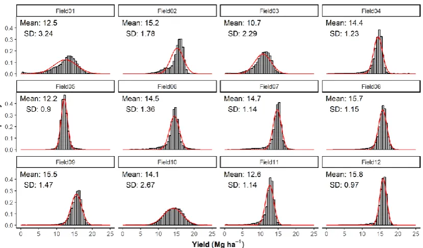
Figure 1. Histograms of corn yield distribution (Mg ha-1) for the 12 fields under the Data
Results and discussion
The histograms of the yield distribution in each field as recorded by the yield monitor (Figure 1) show that the data follow a normal distribution in most situations. Values are concentrated around the mean, and there are more values below the average than would be expected from sampling the normal distribution. This reflects the biological meaning of these values, since many factors can reduce the yields, but increases in yield are limited by the crop’s maximum biological potential. The datasets represent a range of high yielding fields, varying from 10.7 Mg ha-1, slightly lower than the national average of 11.1 Mg ha-1in the 2017 season (United States Department of Agriculture - USDA, 2017),
to 15.8 Mg ha-1. The standard deviation of yield varied from less than 1.0 Mg ha-1 to more than 3.0 Mg ha-1, illustrating differences in field growing conditions.
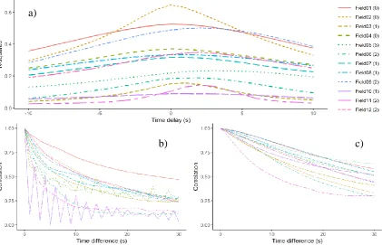
The correlation between PCs and yield was usually higher for the first PC (Table 1), which explains most of the variability. The main exception was field 6, in which the second and third components had the highest absolute value of correlation. The ability of the time series of NDVI images to predict the yield varied among the fields. The best results were observed in field 2, with 75% of the variance explained by the model. The worst performance was observed in field 10, with only 16% of the variance explained by the model. These results are important because the utility of the satellite images to improve the accuracy of the yield maps is directly related to their ability to predict yield. Nevertheless, the low performance of the yield prediction can also be caused by noise in the yield data, and by the inability of the model to capture the underlying relations. Further exploration of the field 10 data revealed that the problem was very likely to be with the yield data itself (Figure 2b).
Table 1. Correlation coefficient between each principal component of the NDVI images and the yield, and the coefficient of determination of the yield prediction using all PCs and the experimental unit polygon identification.
Field PC1 PC2 PC3 PC4 PC5 PC6 R2
1 0.65 -0.20 -0.08 0.08 0.04 -0.04 0.73
2 0.74 -0.12 0.08 0.17 -0.12 0.02 0.75
3 0.38 0.05 0.03 -0.03 0.00 0.08 0.61
4 0.52 0.27 0.32 -0.05 -0.37 -0.23 0.45
5 0.40 0.22 0.05 0.01 0.00 0.08 0.41
6 0.07 -0.29 -0.33 -0.04 0.04 -0.04 0.29
7 0.48 -0.11 -0.16 0.22 0.02 -0.05 0.50
8 0.45 0.34 0.11 -0.01 0.00 0.00 0.48
9 0.45 0.50 -0.11 0.00 0.05 -0.05 0.58
10 0.18 -0.17 0.17 0.00 -0.03 0.00 0.16
11 0.16 -0.23 -0.16 0.01 -0.02 0.08 0.28
12 0.50 0.31 -0.15 0.05 -0.01 -0.03 0.59
other four fields by two seconds, and in one field by three seconds in order to match the yield values with the coordinates (Figure 2a).
Fields 4 and 10 presented noisy data with negative temporal autocorrelation (Figure 2b). The accuracy of the data with these characteristics is questionable. It is likely that a sensor malfunction was the reason for such behavior. Discarding the data, especially for field 10 could be the more reasonable decision. For field 4, aggregating the data every few seconds could be a viable strategy. If the data is aggregated to every experimental unit, the short scale noise introduced by the sensor may not be a problem. The autocorrelation in the yield prediction was usually higher, evidencing that the NDVI variation is smoother than the variability registered by the yield monitor.
The standardized residuals of the yield prediction model were used to identify points with unlikely yield values for that location, as an alternative to the traditional approach of using local statistics without any assumption of spatial dependence or stationarity. The traditional criterion of excluding points outside the range of three times the standard deviation can be applied.
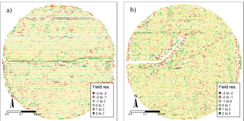
In the two fields chosen as example (Figure 3), most of the errors highlighted with the more intense green and red colors are due to subtle changes in the machine speed or the wrong cutting width. There is no tendency of eliminating points close to the border of the experimental units with different treatments or to consider as erroneous the data points with low yields due to low nitrogen rates, for example. Although the proposed methodology requires the use of additional information, it can be considered simpler than most of the current procedures recommended for yield data filtering (Lyle et al. 2014), avoiding the use of many arbitrarily chosen steps and parameters.
Figure 2. a - Yield prediction performance as function of changing the delay of the yield record. The number inside the parenthesis in the legend represents the time with the highest R-squared. b - Temporal autocorrelation of the yield data observations in each field. c - Temporal autocorrelation of the predicted yield in each field.
a)
The inclusion of other layers in the yield prediction model was also considered, especially the use of variables related to field topography. The use of the satellite images was preferred due to the difficulty of obtaining accurate elevation data for all fields and the possible correlation between the slope of the field and the errors in the yield monitor. The independence of the yield estimation errors and the yield monitor errors was one of the assumptions to identify the presence of artificial trends in the yield data. The trends are defined as the presence of a significant change in the estimated average of the yield in each polygon representing one experimental unit.
Visualizing the standardized estimated coefficient of each polygon as function of the time of harvest can reveal such trends. Because the rates are randomly assigned to the plots, these coefficients should not present any correlation with time. This behavior can be observed in fields 2 and 4 (Figure 4), for example. Various levels of trends can be observed in other fields, from small deviation to the straight line in fields 6 and 12 to large deviations in fields 1 and 5. The spatial distribution of the estimated coefficients for each experimental unit can be used to further investigate these trends (Figure 5). The method used cannot distinguish between trends introduced by data collection and trends related to other management factors that may affect yield without affecting NDVI. Independent of the factor causing the trend, it is important to acknowledge the existence of these trends and to account for it when analyzing the yield response, either by excluding part of the data or including grouping factors.
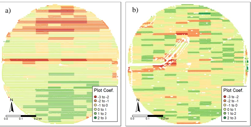
Differences similar to the pattern observed in field 2 (Figure 5a) are expected due to the different treatments in the field and the fact that some factors that affected yield may not have affected NDVI, especially late in the season, when the NDVI gets saturated. Differences such as the ones observed in field 1 (Figure 5b) are unlikely to be caused by the treatment effects in yield. The main stripe of negative values in the middle of the field is clearly an error and should be eliminated. Besides that, there are still three different clusters of errors present in the data. The group of negative values in the north of the field seems to be related to the harvest, since they are mostly aligned with the harvest direction. The group of values in the bottom of the field may be related to irrigation, since it shows a radial distribution.
Figure 3. Spatial distribution of the standardized yield residuals in fields 1 (a) and 2 (b). b)
Figure 4. Standardized coefficients for each experimental unit compared to the relative time of harvest. The blue line represents a smoothed moving average.
The use of an independent sensor to calibrate the load cell at the impact plate, such as a weighing system for the grain tank could contribute to the validation of this methodology. The use of simulation can also be an alternative to validate the proposed methodology (Leroux et al. 2017), but the delays in yield record and the presence of trends should be included in the simulated data.
Figure 5. Spatial distribution of the standardized coefficients for each experimental unit in fields 1 (a) and 2 (b).
Conclusions
The proposed method allowed the identification of the most likely time shift to be applied to correct the yield monitor values. This value varied from zero seconds, meaning that the value set in the monitor configuration was right, to three seconds, meaning that the value set in the yield monitor configuration should be increased by three to better match the sensor readings with the coordinates.
The residuals of the yield prediction model were used to identify points with unlikely yield values for that location, based only on the global frequency distribution of the values. This method can be seen as an alternative to the traditional approaches using local spatial statistics, without any assumption of spatial dependence or stationarity.
The temporal and spatial distribution of the standardized coefficients for each experimental unit highlighted the presence of trends in the data. Although the method cannot explain the reason for the trend, it can help to improve the quality of subsequent analysis by accounting for the trends in the model definition.
Acknowledgements
References
Griffin, T. W., Dobbins, C. L., Vyn, T. J., Florax, R. J. G. M., & Lowenberg-DeBoer, J. M. (2008). Spatial analysis of yield monitor data: case studies of on-farm trials and farm management decision making. Precision Agriculture, 9(5), 269–283. doi:10.1007/s11119-008-9072-2 Houborg, R., & McCabe, M. F. (2018). A Cubesat enabled Spatio-Temporal Enhancement
Method (CESTEM) utilizing Planet, Landsat and MODIS data. Remote Sensing of Environment, 209, 211–226. doi:10.1016/j.rse.2018.02.067
Khanal, S., Fulton, J., Klopfenstein, A., Douridas, N., & Shearer, S. (2018). Integration of high resolution remotely sensed data and machine learning techniques for spatial prediction of soil properties and corn yield. Computers and Electronics in Agriculture, 153, 213–225. doi:10.1016/j.compag.2018.07.016
Leroux, C., Jones, H., Clenet, A., Dreux, B., Becu, M., & Tisseyre, B. (2017). Simulating yield datasets: an opportunity to improve data filtering algorithms. Advances in Animal Biosciences, 8(02), 600–605. doi:10.1017/S2040470017000899
Leroux, C., Jones, H., Clenet, A., Dreux, B., Becu, M., & Tisseyre, B. (2018). A general method to filter out defective spatial observations from yield mapping datasets. Precision Agriculture, 19(5), 1–20. doi:10.1007/s11119-017-9555-0
Lyle, G., Bryan, B. A., & Ostendorf, B. (2014). Post-processing methods to eliminate erroneous grain yield measurements: review and directions for future development. Precision Agriculture, 15(4), 377–402. doi:10.1007/s11119-013-9336-3
Peralta, N. R., Assefa, Y., Du, J., Barden, C. J., & Ciampitti, I. A. (2016). Mid-Season High-Resolution Satellite Imagery for Forecasting Site-Specific Corn Yield. Remote Sensing,
8(10), 1–16. doi:10.3390/rs8100848
Planet Team. (2017). Planet Application Program Interface: In Space for Life on Earth. San Francisco, CA, USA. https://api.planet.com
R Core Team. (2018). R: A Language and Environment for Statistical Computing. Vienna, Austria. https://www.r-project.org/
United States Department of Agriculture - USDA. (2017). Quick Stats 2.0. Washington DC.: U.S.
Department of Agriculture, National Agricultural Statistics Service.