Will Very Large Corpora Play For Semantic Disambiguation The Role That
Massive Computing Power Is Playing For Other AI-Hard Problems?
Alessandro Cucchiarelli*, Enrico Faggioli*, Paola Velardi†
*University of Ancona [email protected]
†
University of Roma "La Sapienza" [email protected]
Abstract
In this paper we formally analyze the relation between the amount of (possibly noisy) examples provided to a word-sense classification algorithm and the performance of the classifier. In the first part of the paper, we show that Computational Learning Theory provides a suitable theoretical framework to establish one such relation. In the second part of the paper, we will apply our theoretical results to the case of a semantic disambiguation algorithm based on syntactic similarity.
1. Introduction
Word sense disambiguation (WSD) is one of the most central and most difficult Natural Language Processing tasks. The problem of WSD is one of identifying the semantic category of an ambiguous word in a sentence context, for example, the financial institution sense on bank in: " A survey by the Federal Reserve's 12 district banks and the latest report by the National Association of Purchasing Management
blurred that picture of the economy."
Linguistic concepts are rather vague - the notion that the word “bank” belongs to such categories as human
organization (the financial institution sense) and
location (the bank-river sense) is more or less intuitive, but in no way it is possible to characterize a linguistic concept in a rigorous way, through a mathematical expression, a logic formula, or a probability distribution.
Linguistic concepts are a convention, and even one on which there is little assent.
A pragmatic approach is to inductively define linguistic concepts as clusters of words sharing some
properties that can be systematically observed in
spoken or written language. A property is a regularity related to the way words are used, or to the internal structure of the entities they represent. A more subjective approach is to discover linguistic concepts using introspection or psycholinguistic experiments. In both cases, the resulting taxonomy, or concept inventory, keeps a considerable degree of “fuzziness”, though it may result an acceptable convention for the purpose of certain interesting tasks. Our perspective here is limited to natural language processing (NLP) by computers, but many fields of science are interested in the study of linguistic concepts.
Given a class C of concepts ci (where C is either a hierarchy or a “flat” concept inventory), the problem of WSD is how to characterize formally a probabilistic or Boolean function that assigns a word w to a concept ci, given the sentence context of w, and (possibly) given some a-priori knowledge.
In the literature (see (CompLing 1998) for some recent results), there is a rather vast repertoire of supervised and unsupervised learning algorithms for WSD, most of which are based on a formal characterization of the surrounding context of a word, a
lexicon of linguistic concepts1 , and a similarity function to compute the membership of a word to a category.
In purely context-based algorithms the idea is that, if a group of words share certain properties, this must be reflected by some observable regularity in the use we make of these words in texts.
Other algorithms use also background knowledge, manually defined using some formal representation language, or automatically extracted through processing of available dictionary definitions.
Despite the rich literature, none of these algorithms exhibit an “acceptable” performance (with reference to the needs of some real-world tasks, e.g. Information Retrieval, Information Extraction, Machine Translation etc.), except for particularly straightforward cases. It is to say that many researchers dispute, in the first place, about the utility of WSD in such applications.
So far the effort of scientists in the area of computational linguistics concentrated on the definition of learning algorithms and on the appropriate balance of contextual and background information, as provided by on-line linguistic resources. What the authors of this article believe is that the problem is not so much with the ideas behind the various learning algorithms, but with the relation between the amount of examples provided to the learner and the complexity of the concept to be learned.
It is fully acceptable, and proved by psycholinguistic experiments, that semantic disambiguation is performed by humans on the basis of a (rather limited) context around the ambiguous word. Though we do not know exactly what mixture of syntactic, morphologic and background semantic knowledge humans use in performing this task, the key to success does not seem to lie only in the appropriate cocktail of these ingredients, but in our wide exposition to examples of language use.
The long lasting objective of our research, whose first results are presented here, is to verify that, similarly, wide exposition to examples will indeed cause a significant performance improvement of context-based WSD algorithm.
Just as the problem of chess game (and other notorious AI-hard problems) has received a considerable improvement also by virtue of mere computing power, we could hope that NLP will experience a similar breakthrough thanks to an analogous "brute-force" approach, that is, the possibility to access millions of examples of language uses. This, by the
1 On-line resources such as WordNet (Miller, 1995) and the
way, is not to be seen as a far future, given the virtually infinite repository of language-in-use samples already available on the WWW.
To prove our intuition it is necessary to establish a
well funded relation between the amount of (possibly noisy) examples provided to a word-sense classification
algorithm and the performance of the classifier.
The hypothesis of noisy learning is necessary, since, while very large example sets can be made available for training, it is not realistic to rely on wide-sized
manually classified examples.
2. Goal of the paper
In the first part of the paper, we will demonstrate that one such dependence can be formally established under the condition that the classification algorithm is a PAC (Probably Approximately Correct) learning (Valiant, 1984). The PAC theory is well established in the area of Computational Learning, however is has not applied so far to the problem of language learning probably because of the difficulty in formally describing linguistic concepts.
In the second part of the paper, we will apply our theoretical results to the case of a semantic disambiguation algorithm based on syntactic similarity2. We will analyze the dependence of performance on the example size, the "vagueness" of the linguistic concept to be learned, and the language domain. Though the limited dimension of our example set (one million words) provides enough evidence only for the study of more contextually characterized concepts (e.g. person
or artifact as opposed to vague WordNet categories
such as psychological_feature), still the behaviour of performance parameters confirms clearly the theoretically derived dependencies.
3. The theory of PAC learning
As we said, the aim of a WSD learning process, when instructed with a sequence S of examples in X, is to produce an hypothesis h which, in some sense, “corresponds” to the concept under consideration.
Because S is a finite sequence, only concepts with a finite number of positive examples can be learned with total success, i.e. the learner can output an hypothesis h= Ci . In general, and this is the case for linguistic concepts, we can only hope that h is a g o o d approximation of Ci.. In our problem at hand, it is worth noticing that even humans may provide only approximate definitions of linguistic concepts!
The theory of Probably Approximately Correct (PAC) learning, a relatively recent field at the borderline between Artificial Intelligence and Information Theory, states the conditions under which h reaches this objective, i.e. the conditions under which a computer derived hypothesis h ‘probably’ represents Ci ‘approximately’.
Definition 1 (PAC learning). Let C be a concept class over X. Let D be a fixed probability distribution
2 The algorithm is an extention of a sense disambiguation
algorithm for proper noun classification, published by Cucchiarelli and Velardi on LREC 98 (Cucchiarelli et al. 1998b).
over the instance space X, and EX(Ci,D) be a procedure reflecting the probability distribution of the population we whish to learn about. We say that C is PAC learnable if there exists an algorithm L with the following property: For every Ci∈C, for every distribution D on X, and for all 0<ε<1/2 and 0<δ<1/2, if L is given access to EX(Ci,D) and inputs ε and δ, then with probability at least (1-δ), L outputs a hypothesis h for concept Ci, satisfying error(h)<ε.
The parameters ε and δ have the following meaning: ε is the probability that the learner produces a generalization of the sample that does not coincide with the target concept, while δ is the probability, given D, that a particularly unrepresentative (or noisy) training sample is drawn. The objective of PAC theory is to predict the performance of learning systems by deriving a lower bound for m, as a function of the performance parameters ε and δ.
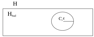
Figure 1: ε-sphere around the “true” function Ci
Figure 1 (from (Russell and Norving, 1999)) illustrates the “intuitive” meaning of PAC definition. After seeing m examples, the probability that Hbad includes consistent hypotheses is:
P(Hbad⊇Hcons)≤| Hbad|(1−ε) m
≤|Η|(1−ε)m
And we want this to be:
|Η|(1−ε)m≤δ
we hence obtain a lower bound for the number of examples we need to submit to the learner in order to obtain the required accuracy:
(1) m≥ ln +ln H
1 1
ε δ
The inequality (1) establishes a sort of worst-case general bound, but unfortunately this bound turns out to have limited utility in practical applications, because it is often difficult to derive a measure for |Η|.
For example, if the hypothesis space for a linguistic concept Ci is the classic “bag of words”, i.e. a set of at least k “typical” context words selected by a probabilistic learner, after observing m samples of the ±n words around words w∈ Ci (e.g. x = (w-n,w-n+1,.. w,…wn-1,wn) ), then h∈H is any choice of 1≤k≤|V| words over at most |V| elements, where |V|=o(≈105) is the size of the vocabulary. In practice, only a limited number of words may co-occur with a word w∈ Ci, however this information is certainly unknown to the learner.
We then can only establish a (very upper) bound:
H V V
k
V V
≤ +
+
+ +
≤ 1
1 2 .... 2
Hbad
Ciε
of extracting positive examples of Ci.
Expression (3) provides the requested relation between size of samples and performance of the method.
Classic methods such as Chernoff bounds (Kearns and Vazirani, 1994) must be applied to obtain good approximations for the probabilities above. Notice however that in order to obtain a given accuracy of probability estimates, Chernoff bounds (as well as other methods) calculte a bound on the number of observed examples. We know however that the acquistion of a statistically representative learning set is particularly complex when instances are language samples, as repeatedly remarked in the reports of Senseval WSD evaluation experiment (Senseval 1998). To simplify probability estimations , we can manipulate expression (3) in order to obtain an accuracy bound, rather than an estimate..
Since in (3.1) (1-φ(i,k))<(1-γ), in (3.2) φ(i,k)<γ, and in (3.3) φ(i,k))≤1, we obtain the upper bound:
(4) P(w’ is misclassified on the basis of f’k)
≤Mi−Ni
(
−)
+ +m
Ni
m m
Mi m
1 γ γ β
The bound (4) can be more easily estimated than expression (3), on the basis of an analysis of the learning corpus submitted to the WSD learner. The objective is to compute a bound for the expected accuracy, as a function of the WSD learning algorithm, and of the language domain and specific semantic category.
If this bound is proved realistic when compared with measured performance, it can be used to tune the WSD experiment parameters, and to derive performance expectations when increasing the size of the learning set.
1 . The probability of false negatives and false positives depends on the threshold γ, on the complexity of the contextual model and adopted notion of context similarity, but also on the features of the corpus and of the learned concept. Certain categories in certain language domains are used in rather repetitive contexts. This means that the number Ni for such categories tent to decrease rapidly with m. After seeing a "sufficient" number of examples, many feature vectors cumulate a high confidence. Other categories may instead require a much wider training, or may result too "vague" to learn a stable contextual model. In this case, it would be wise to replace the category with less coarse hyponims.
2. The probability of unseen depends, clearly, on the complexity of the contextual model and adopted notion of context similarity, but again, there is an unavoidable percentage of rare phenomena that, in a sense, represent the
performance barrier of any language learning
system.
in case contexts are considered similar if, for example, co-occurring words have some common hyperonym. See (Cucchiarelli et al., 1998) for examples.
To conclude, computing the values Mi, Ni, and β as m grows should provide an estimate of expected WSD accuracy on unseen instances, and provide a "trend" of performances as the number of learning samples grows.
Furthermore, the analysis can be made dependent on specific concepts and algorithm parameters (e.g. the threshold γ, the adopted model for a context, the similarity function, etc.).
5. Experimental and estimated bounds
This section provides a preliminary evaluation of the effectiveness of the analysis proposed in previous section.
We performed an experiment of context-based WSD following, with some modifications, the algorithm described in (Cucchiarelli and Velardi, 1998b). In the mentioned paper the context-based algorithm was applied to the case of Named Entities. The modifications have been introduced to adapt the system to the more complex case of common nouns.
We first briefly describe the algorithm and then we apply the analysis of previous section.
Phase 1: A syntactic processing is applied over the corpus.
A shallow parser (see details in Basili et al., 1994) extracts from the learning corpus elementary syntactic
relations such as Subject-Object, Noun-Preposition-Noun,
etc. An elementary syntactic link (hereafter esl) is represented as:
esl(w
j, mod(typei,wk)) where w
j is the head word, wk is the modifier, and typei is the type of syntactic relation (e.g. Prepositional Phrase, Subject-Verb, Verb-Direct-Object, etc.).
In our study, the context of a word x in a sentence S is represented by the esls including x as one of its arguments .
context(x)= esl(x,mod(typei,wk)) or
esl(wj, mod(typei,x))= cx(x,y,ti)
where y = wk or wj
The feature vectors are then here represented by these triples cx(x,y,ti).
Phase 2: For each semantic category Ci6 we collect all the syntactic contexts of words belonging (also to) the category Ci . The population of esls in each category at the end of this step is the Mi value of previous section. For example,
esl(close mod(G_N_V_Act Xerox))
reads: Xerox is the modifier of the head close in a subject-verb (G_N_V_Act ) syntactic relation. If Ci=
group-g r o u p i n group-g, then since Xerox∈Ci, ti=G_N_V_Act and
y=close.
The context cx(Xerox ,close ,G_N_V_Act) is associated to the category group-grouping.
When x is an ambiguous word, it is associated to more than one category, and its weight smoothed accordingly.
6 We select 12 domain-appropriate WordNet hyperonyms,
In a similar way, if the syntactic type is ambiguous (see (Basili et al 1994) for details), a measure of its ambiguity is used to further smooth the weight of the context.
Phase 3(merge): Syntactic contexts in each category Ci are merged if they are identical or if there are at least k contexts with the same syntactic type and words belonging to a common synset. The policy of context generalization is "cautious", as discussed in detail in the refereed paper.
For example, if k=2, the contexts:
cx(Xerox ,close ,G_N_V_Act) and
cx(meeting,terminate, G_N_V_Act
are clustered as:
cx(group-grouping {00246253} G_N_V_Act)
where the second argument is the WordNet identifier for the synset: end, terminate.
When contexts are grouped, their weights are cumulated. We also maintain the information on the number of initial contexts that originated a grouped context.
Phase 4 (pruning): In this phase the objective is to eliminate in each category contexts that do not cumulate a sufficient statistical evidence. For each clustered context k in a category Ci we compute a probabilistic measure of confidence, φ(i,k), not discussed here for sake of space, that depends on the following factors:
• The relative weight of a context in Ci with respect to the other categories. Contexts with a high entropy of probability distributions across categories should be eliminated, because they have a low discrimination power.
• The syntactic and semantic ambiguity of a context. All the three arguments x,y and t of a context may be ambiguous. When contexts are grouped in phase 3, spurious senses tent to be more sparse with respect to the "real" senses, but semantic ambiguity is still pervasive. After Phase 4, each category model h(Ci) includes Mi-Ni contexts, some of which participate in a unique clustered context.
We now describe the experiment.
The objective of the experiment is to measure certain performance parameters of the previously described WSD algorithm, and verify their correlation with the formal analysis of the previous section, specifically, with the bound (4).
It is to say that a wide-scale, completely convincing experiment is extremely demanding, and will take our group busy for quite a long time in the future.
• A first problem is that PAC theory requires that the test set and the learning set are extracted by
a procedure reflecting the same probability
distribution of phenomena than the analyzed
language domain. The difficulty of generating one such test set is well known in computational linguistics, being a problem per
se even the acquisition of an accurately tagged set of examples.
• An accurate estimate of probabilities in (4), though more simple than those in (3), requires a sufficiently large sample to perform cross-validation, or to apply theoretical criteria such as Chernoff bounds.
• Finally, it would be necessary to extend the analysis to more than one algorithm, to several semantic categories with different grain, and to different corpora of possibly very large size.
Having said that, what follows must be taken as a preliminary experiment, with the aim of at least verifying some correspondence of our theoretical analysis with practical results.
Figure 1a and b illustrate (part of) the results of the experiment, briefly described in the figure caption. Figure 1a plots, for four categories and growing corpus dimensions, the value:
(5) 1−
Ni m
γ
This value is the complement of the bound of false negatives, as in (4).
The Recall of the algorithm for each category is computed as:
Rec(Ci)=
true positives
true positives false negatives unknown positive
false negatives
true positives false negatives unknown positive
unknown positive
true positives false negatives unknown positive _
_ _ _
_
_ _ _
_
_ _ _
+ +
=
−
+ +
−
+ +
1
≥1−
−
Ni
m UPi
γ
where UPi is the relative percentage of unknown positives computed for h(Ci).
Therefore Figure 1b and Figure 1a are expected to exhibit similar behavior.
While the estimated bound is not fully consistent with the measured performance (on the other side we mentioned that we could not produce a test set following the same distribution of phenomena as in the learning corpus) it is important to notice that the two sets of curves have a very similar behavior except for Location.