Egocentric Activity Recognition using Histogram Oriented Features and Textural Features

(1)

CSEIT1726120 | Received : 10 Nov 2017 | Accepted : 27 Nov 2017 | November-December-2017 [(2)6: 397-405]

397

Egocentric Activity Recognition using Histogram Oriented

Features and Textural Features

K. P. Sanal Kumar

*1

_{, R. Bhavani}

2

*1Asst. Professor/Programmer, Dept. of ECE, Annamalai University, Tamilnadu, India. 2

Professor, Department. of CSE, Annamalai University, Tamilnadu, India

ABSTRACT

Recognizing egocentric actions is a challenging task that has to be addressed in recent years. The recognition of first person activities helps in assisting elderly people, disabled patients and so on. Here, life logging activity videos are taken as input. There are 2 categories, first one is the top level and second one is second level. In this paper, the recognition is done using histogram oriented features like Histogram of Oriented Gradients (HOG), Histogram of optical Flow (HOF) and Motion Boundary Histogram (MBH) and textural features like Gray Level co-occurrence Matrix (GLCM) and Local Binary Pattern (LBP). The features like Histogram of Oriented Gradients (HOG), Histogram of optical Flow (HOF) and Motion Boundary Histogram (MBH) are combined together to form a feature (Combined HHM). The extracted features are fed as input to Principal component Analysis (PCA) which reduces the feature dimensionality. The reduced features are given as input to the classifiers like Support Vector Machine (SVM), k Nearest Neighbor (kNN) and Probabilistic Neural Network (PNN). The performance results showed that SVM gave better results than kNN and PNN classifier for both categories.

Keywords: Egocentric: Histogram Oriented; Textural; Principal Component Analysis; Life Logging Activity

I. INTRODUCTION

Recognizing human actions from videos is a trend in computer vision. The advancement of wearable devices has led the trend to identify actions from such videos. These videos are egocentric videos which means self-centered. The term egocentric defines that it is concerned with an individual rather than the society. Analysing the activities of a person is to help the elderly people, people who are disabled, patients and so on [1].

In the welfare field, there are several categories in domestic behaviours, which are identified as ADL (activity in daily living). A home monitoring system gives a one-day analysis on ADL to monitor the user’s lifestyle. ADL is also used for special health care which improves one’s strength both physically and mentally. Nowadays, glass-type camera devices have been given for users, which extends its applications into his/her daily life as well. One study on activity analysis in daily life [2] identifies all objects from the egocentric videos. This taxonomy defines the user’s

behaviour. For instance, if “a TV”, “a sofa” and “a remote” are the objects in a frame, this circumstance can be defined as “watching TV”. This method categories each distinguished object into an “active object” or “passive object” based on whether the consumer manipulates the object or not[3]. “Active object” is considered a key object in activity estimation. However, the above method has an inevitable issue, that is, there is a limitation on applicable scenes and object types [4-14]. In this research work, Histogram oriented features like HOG (Histogram of oriented gradients), HOF (Histogram of optical flow) and MBH (Motion Boundary Histogram) are extracted. These features are combined together to form a feature (Combined HHM). Textural features like Gray Level co-occurrence Matrix (GLCM) and Local Binary Pattern (LBP) are also extracted.

II. RELATED WORKS

(2)

complex kitchen activities. Recently, ADL analysis is implemented by exploiting RGB-D sensors [16]. Here, the performance is improved based on cameras which are traditional. A kitchen environment is chosen in [17]. The issues in analyzing human behaviour from wearable camera’s data are represented in [18– 22]. In [18] some features were pointed which depends on the output of multiple object detectors. [19] implemented a method for isolating social interactions in egocentric videos obtained in social events. Office environment is taken egocentric activity recognition where, motion descriptors are extracted which are combined with user eye movements. Some latest works have considered different environments like kitchen, office, etc. [20] proposed codebook generation for a kitchen environment which reduces the problem provided by different styles and speed between different subjects. In [21] an approach is implemented for identifying anomalous events from the chest mounted camera videos. [22] presented a video summarization method targeted to FPV. In [23], multi-channel kernels were investigated to combine local and global motion information. This created a new activity identification method that models the temporal structures of First Person Video data. [24] used First Person Videos which are temporally segmented into twelve hierarchical classes. Here, the FPV ADL analysis is implemented for multi-task learning framework. [25] implemented texture feature extraction using GLCM feature. [26] illustrated the LBP feature for feature extraction from fingerprint image.

PROPOSEDWORK

Figure 1. The Proposed model

The system implemented here has the following steps in training phase.

1. The input video is fed where the feature extraction is applied.

2. The Histogram based features like HOG (Histogram of oriented gradients), HOF (Histogram of optical flow) and MBH (Motion Boundary Histogram) are extracted. The extracted features are concatenated together to form combined HHM (HOG, HOF,MBH).The Textural based features like Gray Level Co-occurrence Matrix (GLCM) and Local Binary Pattern (LBP) are also extracted.

3. The extracted features are fed as input to Principal component Analysis (PCA) which reduces the feature dimensionality.

4. The reduced features are fed to the classifiers like Support Vector Machine (SVM), k Nearest Neighbor (kNN) and Probabilistic Neural Network (PNN).

5. The activity recognition is obtained as output. The above steps are repeated with the testing phase where the input is a query video.

Figure 1 depicts the flow diagram for the proposed model.

III. FEATURE EXTRACTION

3.1 Histogram of Oriented Gradients (HOG)

Figure 2. Feature Extraction diagram for HOG Apply Normalization for gamma and color

values

Compute the gradient values

Assign weights for both spatial and orientation cells

Apply Normalisation for overlapping blocks

(3)

This feature is local shape information described by the distribution of gradients or edge directions. This generally focuses on static appearance information [27]. The input frame is chosen where the normalization is applied on both color values and gamma correction is applied. The next step is to apply gradient filter for finding the gradient values. Divide the window into adjacent, non-overlapping cells of size C×C pixels (C = 8). In each cell, compute a histogram of the gradient orientations binned into B bins [28].

Calculate the weights by using bilinear interpolation. These are subjected to normalization by concatenating overlapping blocks.

The normalized block features are concatenated into a single feature vector which is the HOG.

Initially the videos are divided into frames and then the feature extraction is applied.

Figure 2 depicts the flow diagram for HOG feature extraction. Here, the size of the HOG feature is 8102.

3.2 Histogram of Optical Flow (HOF)

In video domain, optical flow is commonly known as the apparent motion of brightness patterns in the images [29]. An optical flow vector is defined for a point (pixel) of a video frame. In optical flow estimation of a video frame, selection of “descriptive” points is important. This selection is done using visual features. Here, the size of the HOF feature is 2050.

Figure 3. Flow diagram for HOF

3.3 Motion Boundary Histogram (MBH)

Optical flow represents the absolute motion between two frames, which contains motion from many sources, i.e., foreground object motion and background camera motion. If camera motion is considered as action motion, it may corrupt the action classification. Various types of camera motion can be observed in realistic videos, e.g., zooming, tilting, rotation, etc. In many cases, camera motion is translational and varies smoothly across the image plane. [30] proposed the motion boundary histograms (MBH) descriptor for human detection by computing derivatives separately for the horizontal and vertical components of the optical flow. The descriptor encodes the relative motion between pixels. Since MBH represents the gradient of the optical flow, locally constant camera motion is removed and information about changes in the flow field (i.e., motion boundaries) is kept. MBH is more robust to camera motion than optical flow and thus more discriminative for action recognition. The MBH descriptor separates optical flow ω= (u, v) into its horizontal and vertical components. Spatial derivatives are computed for each of them and orientation information is quantized into histograms. The magnitude is used for weighting. We obtain a 8-bin histogram for each component. Compared to video stabilization [31, 32] and motion compensation [33], this is a simpler way to discount for camera motion. The MBH descriptor is shown to outperform significantly the HOF descriptor in our experiments. For both HOF and MBH descriptor computation, we reuse the dense optical flow that is already computed to extract dense trajectories [34]. This makes our feature computation process more efficient. Here, the size of the MBH feature is 2050.

3.4 Combination of features (Combined HHM) In this article, the features are concatenated into a single feature vector i.e., the HOG, HOF and MBH are fused together. The HOG feature vector contains 8102 features, HOF has 2050 features and MBH has 2050 features. All these features are combined together 12202 features.

3.5 GLCM

Gray-level co-occurrence matrix (GLCM) is the statistical technique for texture based analysis that uses the spatial relationship of the pixels. The GLCM functions obtain the texture of an image by ascertaining Video with

optical flow

Quantize the orientation of

optical flow vectors

Compute the optical flow and their differential

optical flow vectors Calculate the

histograms of each subregion optical

flow

Concatenate the flow histograms of subregions to form

(4)

how frequently pairs of pixel with specific values and in a spatial relationship occur in an image. This creates a GLCM which extracts statistical measures from this matrix. The gray-level co-occurrence matrix (GLCM) which is a matrix, is calculated by computing the occurrence of a pixel with the intensity (gray-level) value i in a specific spatial relationship to a pixel with the value j. Each element (i, j) in the resultant GLCM is the total of the number of times that the pixel with value i occurred in the specified spatial relationship to a pixel with value j in the input image [24].

The local binary pattern (LBP) encodes the relationship between the referenced pixel and its surrounding neighbors by computing difference in gray-levels [25]. The Local Binary Pattern is implemented for texture classification. It contains at most two bitwise transitions from 0 to 1 or vice versa.

Algorithm for LBP Feature Extraction

Step 1: Divide the video into frames where each frame is partitioned into 3x3 window

Step 2: Partition the examined window into cells. Step 3: For every single value in the cell, compare the

pixel value with that of the centre pixel’s value.

Step 4: If the value of the center pixel is greater than that of the neighbor pixel value then assign 1. Else assign 0 using the equation (16).



centre pixel value and its neighbor.

Step 5: The LBP code is calculated as Step 6: Calculate the histogram based on the frequency

of each number in the cell.

Step 7: Concatenate normalized histograms.

This provides the feature vector. In our research work, there are 102 features for each frame.

3.7 DIMENSIONALITY REDUCTION USING PRINCIPAL COMPONENT ANALYSIS (PCA)

The obtained feature vectors are of large size. This large dimension results in a very slow computation. As a result, the dimensions are reduced using Principle Component Analysis.

In statistics, Principal Components Analysis (PCA) [35] is a technique which is implemented to decrease the dimensionality of a high dimensional data set. It is a linear transformation that chooses a new coordinate system for the data set. The new coordinate system is a representation of the directions where the variance of the data is high. The PCA can be used for reducing dimensionality in a data set while retaining the attributes of the data set that contribute most to its variance, by retaining lower-order principal components and ignoring higher-order ones.

Applying Principal Component Analysis

Algorithm for PCA

Step 1: Generate the column vectors from the input feature vectors.

Step 2. Calculate the covariance matrix of the two column vectors that is formed in step1.

Step 3. The variance of each column vector is obtained from the diagonal elements of the 2×2 covariance vector with itself, respectively.

Step 4. Compute the Eigen values and the Eigenvectors of the covariance matrix [36].

(5)

features. In case of textural features, GLCM feature size is reduced to 5 and LBP feature size is reduced to 30.

IV. CLASSIFIERS

4.1 Support Vector Machine

In machine learning, support vector machines are models that are associated with learning algorithms for analyzing and classifying data. An SVM algorithm creates a model that assigns examples to one category or another. This model maps the examples which divide into the separate categories [38]. New examples are trained to assign into categories already divided and they are predicted. In addition to performing linear classification, SVMs can efficiently perform a non-linear classification. Here multiclass SVM is used.

Figure 4: Support Vector Machine

Figure 4 shows the separation of examples using optimal hyperplane which is cited from [39]. The operation of SVM is based on the hyperplane that gives largest minimum distance to the training examples.The output is activity recognition for 5 top level categories and 13 second level categories.

4.2 kNN Classifier

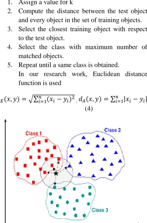
The kNN is k-Nearest Neighbor which is supervised algorithm. Here, the result is classified based on majority of k-Nearest Neighbor category. This algorithm classifies a new entity based on attributes and training samples. This algorithm uses neighbourhood for classification as the prediction value of the new example. Figure 5 depicts the kNN classifier which separates the objects into different classes. This is cited from [40].

Steps in kNN classifier algorithm: 1. Assign a value for k

2. Compute the distance between the test object and every object in the set of training objects. 3. Select the closest training object with respect

to the test object.

4. Select the class with maximum number of matched objects.

5. Repeat until a same class is obtained.

In our research work, Euclidean distance function is used

√∑ , ∑ | |

(4)

Figure 5: kNN classifier for a vector where k value is 5

The output is activity recognition for 5 top level categories and 13 second level categories.

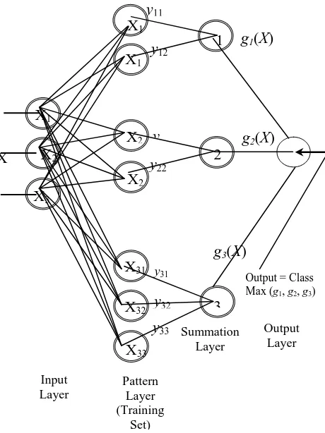
4.3 Probabilistic Neural Network:

The PNN architecture contains many interconnected neurons in successive layers [41]. The input layer unit does not compute and simply distributes the input values to the neurons in the next layer which is the pattern layer. When a pattern x from the input layer xis received, its output is calculated from the pattern layer neuron.

  

 

  



 _ _

 

2 2

) ( ) ( exp

2 ) 2 (

1 )

(

 



 x xij

T ij x x

d d x

ij (5)

(6)

Figure 6: Architecture of Probabilistic Neural Network The summation layer neurons calculate the maximum likelihood of pattern x which is classified into ci. The output of all neurons are summarized and averaged which belongs to the same class [42].

 class Ci. If the apriori probabilities for each class have the same value and the losses for making an incorrect decision for each class are equal, the decision layer classifies the pattern with respect to the Bayes’s decision rule which is based on the output of all the summation layer neurons.

n

pattern x and m denotes the total number of classes in the training data. Figure 3 depicts the architecture of

Probabilistic Neural Network. Each image has a combination of specific values of the input vector which is called an input pattern that describes the features of the image.

In the input layer, the number of input features is equal to the number of neurons. In the pattern layer, the total number of neurons is defined as the sum of the number of neurons which represents the patterns for each category.The output layer contains nodes for each pattern classification. The sum for each hidden node is propagated to the output layer where the highest value wins.

V. PERFORMANCEMETRICS

Accuracy is defined as the ratio between the summation of true positive rate and true negative rate and the total population.

Accuracy = Tp+Tn / (Tp+Tn+Fp+Fn) (8) where,

Tp is the number of data classified correctly as positive class

Tn is the number of data classified correctly as negative class

Fp is the number of data classified wrongly as positive class

Fn is the number of data classified wrongly as negative class phone, talk to people, watch videos, use internet, write, read, eat, drink and housework. Table 1 shows the accuracy of both classifiers for top level.

Table 1: Accuracy for top level categories

(7)

0 20 40 60 80 100

SVM kNN PNN

HOG

HOF

MBH

Combined HHM

GLCM

LBP

Table 2: Accuracy for second level categories

Features

Classifiers

Histogram of Oriented Gradients

Histogram of Optical

Flow

Motion Boundary Histogram

Combined

HHM GLCM LBP

SVM 69.23 77.14 79.54 85.54 87.32 83.13 kNN 64.34 71.56 73.21 79.83 81.97 77.65 PNN 66.59 74.83 77.32 82.75 84.67 78.15

Figure 7: The chart to depict accuracy for top level categories

In the above table and figure, SVM classifier provides 80.25% for HOG, 84.38% for HOF, 85.56% for MBH, 89.47% for combined HHM, 91.35% for GLCM and 82.28% for LBP of accuracy for top level categories which are higher than kNN and PNN classifiers. Therefore, SVM classifier with GLCM performs better than kNN and PNN classifiers. Table 2 depicts the accuracy of both classifiers for second level.

Figure 7: The chart to depict accuracy for second level categories

In the above table and figure, SVM classifier provides 69.23% for HOG, 77.14% for HOF, 79.54% for MBH, 85.54% for combined HHM, 87.32% for GLCM and 83.13% for LBP of accuracy for second level categories which are higher than kNN and PNN classifiers. Therefore, SVM classifier with GLCM performs better than kNN and PNN classifiers.

VII. CONCLUSION

In this research article, SVM classifier with GLCM provided better results than kNN and PNN classifiers. SVM provides advantages like it is accurate and robust even when the training sample has some bias. It delivers unique solution since the optimality problem is convex. Therefore SVM classifier with GLCM provided better results.

VIII. REFERENCES

[1] Kenji Matsuo, Kentaro Yamada, Satoshi Ueno, Sei Naito, “An Attention-based Activity Recognition for Egocentric Video”, IEEE Conference on Computer Vision and Pattern Recognition, 2014.

[2] H. Pirsiavash and D. Ramanan, “Detecting activities of daily living in first-person camera views”, IEEE Conference on Computer Vision and Pattern Recognition, 2012.

[3] Sanal Kumar, K.P. Bhavani, R. and M. Rajaguru, Egocentric Activity Recognition Using Bag of Visual Words, International Journal of Control Theory and Applications, Vol.9, Issue 3, pp. 235-241, 2016.

[4] M. Cerf, J. Harel, W. Einhauser, and C. Koch. Predicting human gaze using low-level saliency combined with face detection. Advances in Neural Information Processing Systems (NIPS), Vol. 20, pp. 241-248,2007.

[5] L. Itti, N. Dhavale, F. Pighin, et al. Realistic avatar eye and head animation using a neurobiological model of visual attention. In SPIE 48th Annual International Symposium on Optical Science and Technology, Vol. 5200, pp. 64-78, 2003.

[6] J. Harel, C. Koch, and P. Perona. Graph-based visual saliency. Advances in Neural Information Processing Systems (NIPS), Vol. 19, pp. 545-552, 2006.

[7] C. Koch and S. Ullman. Shifts in selective visual attention: towards the underlying neural circuitry. Human Neurobiology, Vol. 4, No. 4, pp. 219-227, 1985.

70 72 74 76 78 80 82 84 86 88 90

SVM kNN PNN

Acc

ura

cy

Classifiers

(8)

[8] L. Itti, C. Koch, and E. Neibur. A model of saliency-based visual attention for rapid scene analysis. IEEE Transactions on Pattern Analysis and Machine Intelligence (PAMI), Vol. 20, No. 11, pp. 1254-1259, 1998.

[9] T. Avraham and M. Lindenbaum. Esaliency (extended saliency); Meaningful attention using stochastic image modeling. IEEE Transactions on Pattern Analysis and Machine intelligence (PAMI), Vol. 32, No. 4, pp. 693-708, 2010. [10] L. F. Coasta. Visual saliency and attention as

random walks on complex networks. ArXiv Physics e-prints, 2006.

[11] W. Wang, Y. Wang, Q. Huang, and W. Gao. Measuring visual saliency by site entropy rate. In Computer Vision and Pattern Recognition (CVPR), pp. 2368-2375, IEEE, 2010.

[12] T. Foulsham and G. Underwood. What can saliency models predict about eye movements? Spatial and sequential aspects of fixations during encoding and recognition. Journal of Vision, Vol. 8, No. 2;6, pp. 1-17, 2008.

[13] M. Cheng, G. Zhang, N. Mitra, X. Huang, and S. Hu. Global contrast based salient region detection. In IEEE Conference on Computer Vision and Pattern Recognition (CVPR), 2012. [14] K. Yamada, Y. Sugano, T. Okabe, Y. Sato, A.

Sugimoto, and K. Hiraki. “Attention prediction in egocentric video using motion and visual saliency,” in Proc. 5th Pacific-Rim Symposium on Image and Video Technology (PSIVT) 2011, vol.1, pp. 277–288, 2011.

[15] R. Messing, C. Pal, and H. Kautz, “Activity recognition using the velocity histories of tracked key points,” in IEEE International Conference on Computer Vision, 2009.

[16] J. Lei, X. Ren, and D. Fox, “Fine-grained kitchen activity recognition using RGB-D,” in ACM International Joint Conference on Pervasive and Ubiquitous Computing, 2012.

[17] M. Rohrbach, S. Amin, M. Andriluka, and B. Schiele, “A database for fine grained activity detection of cooking activities,” in IEEE Conference on Computer Vision and Pattern Recognition, 2012.

[18] H. Pirsiavash and D. Ramanan, “Detecting activities of daily living in first-person camera views,” in IEEE Conference on Computer Vision and Pattern Recognition, 2012.

[19] K. Ogaki, K. M. Kitani, Y. Sugano, and Y. Sato, “Coupling eye-motion and ego-motion features for first-person activity recognition,” in CVPR Workshop on Egocentric Vision, 2012.

[20] E. Taralova, F. De la Torre, and M. Hebert, “Source constrained clustering,” in IEEE International Conference on Computer Vision, 2011.

[21] A. Fathi, Y. Li, and J. M. Rehg, “Learning to recognize daily actions using gaze,” in European Conference on Computer Vision, 2012.

[22] A.Fathi, A. Farhadi, and J. M. Rehg, “Understanding egocentric activities,” in IEEE International Conference on Computer Vision, 2011.

[23] M. S. Ryoo and L. Matthies, “First-person activity recognition: What are they doing to me?” in IEEE Conference on Computer Vision and Pattern Recognition, 2013.

[24] Y. Poleg, C. Arora, and S. Peleg, “Temporal segmentation of egocentric videos,” in IEEE Conference on Computer Vision and Pattern Recognition, 2014.

[25]P. Mohanaiah, P. Sathyanarayana,L. GuruKumar, “Image Texture Feature Extraction Using GLCM Approach”, vol.3, no.5, May 2013.

[26]Zhihua Xia, Chengsheng Yuan, Xingming Sun, Decai Sun, RuiLv, “ Combining Wavelet Transform and LBP Related Features for Fingerprint Liveness Detection” , IAENG International Journal of Computer Science, vol.43, no.3, August 2016.

[27] Kishor B. Bhangale and R. U. Shekokar, “Human Body Detection in static Images Using HOG & Piecewise Linear SVM”, International Journal of Innovative Research & Development, vol.3 no.6, (2014).

[28] Sanal Kumar, K.P. and Bhavani, R., Egocentric Activity Recognition Using HOG, HOF and MBH Features, International Journal on Recent and Innovation Trends in Computing and Communication, vol. 5 no. 7, pp.236 – 240. [29] Sri Devi Thota, Kanaka Sunanda Vemulapalli

,Kartheek Chintalapati, Phanindra Sai Srinivas Gudipudi, “Comparison Between The Optical Flow Computational Techniques”, International Journal of Engineering Trends and Technology, vol 4. no.10, 2013.

(9)

appearance,” in European Conference on Computer Vision, 2006.

[31] Sanal Kumar, K.P. and Bhavani, R., Egocentric Activity Recognition Using HOG, HOF, MBH and Combined features, International Journal on Future Revolution in Computer Science & Communication Engineering, vol. 3 no. 8, pp. 74 – 79.

[32] N. Ikizler-Cinbis and S. Sclaroff, “Object, scene and actions: combining multiple features for human action recognition,” in European Conference on Computer Vision, 2010.

[33] H. Uemura, S. Ishikawa, and K. Mikolajczyk, “Feature tracking and motion compensation for action recognition,” in British Machine Vision Conference, 2008.

[34] Sanal Kumar K.P. and Bhavani R, “Activity Recognition in Egocentric video using SVM, kNN and Combined SVMkNN Classifiers”, IOP Conf. Series: Materials Science and Engineering 225, 012226, 2017.

[35] AlirezaSarveniazi, “An Actual Survey of Dimensionality Reduction” American Journal of Computational Mathematics, vol.4, pp.55-72, 2014.

[36] S.Anu H Nair, P.Aruna, “Image Fusion Techniques For Iris And Palm print Biometric System”, Journal of Theoretical and Applied Information Technology, vol. 61, no.3, pp.476-485, 2014.

[37] ArunGarg, Richika, “A Novel Approach for Brain Tumor Detection Using Support Vector Machine, K-Means and PCA Algorithm”, International Journal of Computer Science and Mobile Computing, vol.4, no.8, pp. 457-474, 2015.

[38] M.Suresha, N.A. Shilpa and B.Soumya, “Apples Grading based on SVM Classifier”, in National Conference on Advanced Computing and Communications, 2012.

[39] OpenCV-Introduction to Support Vector Machines.

http://docs.opencv.org/2.4/doc/tutorials/ml/introd uction_ to_svm/introduction_to_svm.html Accessed: 2016-07-22.

[40] Wanpracha Art Chaovalitwongse, Ya-Ju Fan, Rajesh C. Sachdeo, “On the Time Series K-Nearest Neighbor Classification of Abnormal Brain Activity”, IEEE Transactions on Systems,

Man, and Cybernetics – Part A: Systems and Humans, vol.37, no.6 , 2007.

[41] Sanal Kumar, K.P. and Bhavani, R., “Human activity recognition in egocentric video using PNN, SVM, kNN and SVM+kNN classifiers”, Cluster Computing, 2017.