Volume 2006, Article ID 26145, Pages1–20 DOI 10.1155/ASP/2006/26145
The Hermite Transform: A Survey
Jean-Bernard Martens
Department of Industrial Design, Eindhoven University of Technology, Den Dolech 2, P.O. Box 513, 5600 MB Eindhoven, The Netherlands
Received 24 August 2004; Revised 23 November 2004; Accepted 15 January 2005
With this survey on the Hermite transformation we want to pursue the following two goals. First, we want to provide a compre-hensive and up-to-date description of the Hermite transformation, its underlying philosophy, and its most important properties and their implications for applications. As so often when publications and development go hand-in-hand, new insights have led to changes in or generalizations of already published results, and not all of these changes have been considered sufficiently substantial to be published separately. As a consequence, the existing publications on the Hermite transformation do not fully reflect our most recent insights, and the current paper intends to remedy this. Second, we also want to share some new results. Two specific new results, that is, partial signal decompositions and intersection curvatures, are therefore treated in more detail than other aspects.
Copyright © 2006 Hindawi Publishing Corporation. All rights reserved.
1. INTRODUCTION
The Hermite transformation was introduced about 15 years agothrough two related publications [1,2]. It was originally developed to provide a mathematical model for interpreting receptive fields in the early stages of (human) spatial vision [2,3]. It was however also one of the first instances where an overcomplete signal representation was considered for appli-cations. This early belief in the potential benefits of overcom-plete representations, which was motivated by our belief in the superior characteristics of the human visual system, has since been shared by an increasing number of researchers. The acceptance of the Hermite transformation has grown due to demonstrated applications in diverse areas such as image coding [4–6], image fusion [7,8], motion estimation (optic flow) [9,10], image processing [11–15], image param-eter estimation with applications in image quality prediction [16–19], image analysis [20], image indexing [21,22], and modelling of the human visual system [23–25]. The Her-mite transformation has recently also been extended to more than two dimensions using the framework of Clifford analy-sis [26].
The Hermite transformation is an example of an over-complete signal representation, or signal decomposition. It is an invertible mapping of the original signal (specified by its sample values) to an alternative representation. The potential benefit of such alternative representations is that they make different characteristics of the signal explicit and hence acces-sible for processing or coding. The interest in a specific sig-nal representation is therefore determined by its usefulness
in applications. The recent signal-processing literature shows a fast growth, under the impulse of wavelet transformation [27,28] and frame [29] theories, of available signal decom-positions. It seems that there are endless alternatives for ana-lyzing and resynthesizing a signal, and indeed there are. Ob-viously, the demand of global correspondence, that is, that analysis followed by synthesis results in the original signal, is not very restrictive. There is therefore ample room for im-posing additional demands on signal decompositions. In this paper, we specifically consider signal decompositions from the point of view of applications in adaptive image process-ing (and codprocess-ing). We argue that these applications are greatly simplified if signal decompositions have the additional prop-erty oflocal correspondence, that is, if signals can be locally re-covered from the decomposition, using only the coefficients at the position where processing is required. The Hermite transformation is a specific example of such a local signal de-composition, but one with some very useful extra features.
Cp
l(x) A [ln(p)] T(Cp) [ln(p)] S l(x)
Figure1: Algorithmic structure for adaptive image processing with local image decompositions. In the analysis stepA, the input image
l(x) is transformed into a set of coefficients [ln(p)], wherenindexes the different templates andpthe different positions. The coefficients
[l]p=[ln(p),∀n] at a given positionpundergo a transformationT(Cp). The control variablesCpat positionpare derived from [l]pand are used to select the desired transformationT. The transformed coefficients [ln(p)] are combined in the synthesis stepSto obtain the processed
imagel(x).
approximately the same size. The extension to basic func-tions of substantially different sizes can be accomplished by extending the signal decomposition to a multiresolution scheme, that is, by incorporating it in a pyramid structure [1,11,28,30] or in a scale-space setting [31–34]. The weights of the basic functions can be assembled according to tem-plate (i.e., the weights for all positions of a given temtem-plate) or according to position (i.e., the weights for all templates at a given position). In the second stage of the adaptive al-gorithm ofFigure 1, the coefficients are assembled according to position. The original coefficients at a given position are interpreted and mapped (byT) into processed coefficients. Since only coefficients at the same position are combined, this mapping can easily be made to vary across positions. To implement this adaptivity, we derive at each position one or more control variablesCpthat determine which (possibly nonlinear) transformationThas to be applied to the coeffi -cients at that position. These control variables are intended to measure changes in the image itself (e.g., uniform versus edge region, or variable orientation), or changes in the degra-dation (e.g., level-dependent noise such as Poisson noise), so that an adequate transformation can be selected. An image decomposition that allows the image to be reconstructed lo-cally obviously allows any desired local property to be de-rived. Some important local features that will be introduced later are the local average, the local energy (or contrast), the local dimensionality, and the local orientation. In the syn-thesis stageSof the adaptive processing algorithm, the pro-cessed coefficients are applied to their respective basic func-tions. The weighted sum is the processed output image.
InSection 2, we formalize the concept of local signal de-compositions. We show how the idea of performing identi-cal measurements at regular intervals leads to the definition of filters and filter banks. Next, in Section 3, we introduce partial signal decompositions as a specific case of local signal decompositions where the number of required filter opera-tions can be substantially reduced. It is shown inSection 4 how the simplest instance of such a partial signal decom-position, called residue-image processing [15], can be ap-plied for noise reduction and contrast enhancement. Start-ing fromSection 5, we focus on one specific case of local de-compositions, that is, the Hermite transformation for two-dimensional signals [1,2,13]. We define the Hermite trans-formation and show how the mapping between the image and the Hermite coefficients can be implemented. We also
discuss some important properties of the Hermite transfor-mation. Next, inSection 6, we show how local coordinate axes that are oriented along an image-dependent direction can be created. Many geometric image features, such as the isophote and flow-line curvatures and the newly-introduced intersection curvatures, are most easily expressed in a coor-dinate system, that is, oriented along the gradient direction. These geometric features are discussed inSection 7, and it is shown how they can be used to identify conspicuous details (such as corners, junctions, extrema, etc.) in images. Such de-tails are for instance well suited for performing image match-ing, such as that required for stereo vision and motion esti-mation. InSection 8we apply the concept of partial signal decompositions to the Hermite transformation in order to devise an anisotropic noise-reduction algorithm.
2. LOCAL SIGNAL DECOMPOSITIONS
We assume that the input signalsl(x) are defined for a (com-pact) subset F of the D-dimensional Euclidean space RD. This subsetFcan be either continuous or discrete. In the case of image processing, the dimensionD=2, for static images, orD = 3, for image sequences. We assume that the image analysis is linear and hence consists of bounded linear func-tionals [24], that is, linear mappings from the input signal l(x) to the finite real/complex numbers that can be expressed as the inproduct between a test functionφ(x) and the input functionl(x). We moreover assume that this inproduct can be expressed as an integral
φ(x),l(x)=
Fφ(x)·l(x)dx, (1)
in case of continuous signals, or as a sum
φ(x),l(x)=
F
φ(x)·l(x), (2)
in case of discrete signals. The space of test functions that we consider for analyzing the image is denoted byV. Test functions are very often Schwartz functions (smooth local-ized functions) [35]. The signal space contains those signals that result in finite measurements for all test functions inV, and is hence equal to the dual spaceVof bounded linear functionals onV.
[l(x),x∈F] ∗an(−x) ↓P [ln(p),p∈P]
Figure2: Mapping from the input image [l(x), x∈F] to the coefficients [ln(p), p∈P] of ordern, depicted as a two-stage process. The
standard notations∗and↓are used to denote the convolution and (down-)sampling operations, respectively.
w(x) has limited support, so thatw(x−p) is zero except in the neighbourhood of sampling positionp ∈ P. The win-dowed signall(x)·w(x−p) is therefore localized around positionp∈P. The setP contains all positionspon a reg-ular latticeΛ[36] for whichw(x−p) overlaps withF, that is, w(x−p)=0 for at least one coordinatex∈F.
Each of the windowed signalsl(x)·w(x−p) can be de-composed into a sum of orthonormal basis functionsϕn(x−
p)·w(x−p),n∈N, such that
w(x−p)
l(x)−
n∈N
ln(p)·ϕn(x−p)
=0, (3)
where the coefficients are obtained via
ln(p)=
an(x−p),l(x)
=
Fan(x−p)·l(x)dx, (4)
forn∈N andp∈P (equality in (3) actually means con-vergence in the mean-square sense) [20,24]. The (discrete) setN indexes the basis functions. The function
an(x)=ϕn(x)·w2(x) (5)
is referred to as theanalysis functionof ordern. The mapping between the original signall(x) and the coefficients [ln(p)] for all ordersnand positionspspecifies the analysis stageA ofFigure 1.
If measurements are performed at all positions, then (4), taken over all positionsp ∈ RD, defines a D-dimensional
convolutionorfilteringbetween the input signall(x) and the filter with impulse response an(−x), or equivalently, a
cor-relationbetween the input signall(x) and the analysis func-tionan(x). Only a limited number of these output values are however required, sinceP ⊂RD. This operation of selecting a subset of values is called (down-)sampling. The combined operation is depicted inFigure 2. The complete signal analy-sisAcontains several of these filter/sampling combinations, that is, one for each indexn∈ N, and is called amultirate filter bank. The term multirate refers to the fact that the do-mainFon which the original signal is defined is usually dif-ferent from the domainP on which the filter coefficients are required.
There is no unique way of reconstructing the signal l(x) from the coefficients [ln(p);n∈N, p∈P] since any weighted summation
l(x)= p∈P
n∈N
ln(p)·rn(x−p), (6)
with
rn(x−p)=ϕn(x−p) w(x−p)u(x−p)
q∈Pw(x−q)u(x−q), (7)
for which
p∈P
w(x−p)u(x−p)=0, (8)
for all argument valuesx ∈F, is for instance valid. The rea-son why there is no unique reconstruction is that the coeffi -cients of the local signal decomposition are not independent if the window functionsw(x−p) at neighboring positionsp are overlapping. This means that, although there is a unique set of coefficients [ln(p); n∈N,p∈P] for any signall(x), there are many sets of coefficients that do not correspond to a signal. Hence, the set of physically realizable coefficients is a subspace of the space of all coefficients.
To arrive at a unique solution foru(x), we have to in-troduce an additional condition for the reconstruction. One obvious condition is described in the mathematical theory of frames [29]. If we reconstruct a signal from a set of co-efficients that are not physically realizable, and subsequently analyze this signal, then we require the output coefficients to be the closest realizable set of coefficients. In mathematical terms, we impose that synthesisSfollowed by analysisAis equivalent to an orthogonal projectionP = A·Sonto the set of realizable coefficients. This is a useful property in our application since the processed coefficients in adaptive signal processing cannot be guaranteed to be realizable; it is there-fore important to design the synthesis stage such that the co-efficients of the output signal are automatically mapped onto the closest realizable coefficients.
To find the unique reconstruction (synthesis) satisfying the above condition for the given set of analysis functions, we have to determine the frame operatorFawhich maps any signall(x) to the corresponding signal
Fal(x)=
p∈P
n∈N
ln(p)·an(x−p), (9)
forx ∈ F, that arises by also using the analysis functions to perform the signal reconstruction [29]. In the case under consideration, the frame operator reduces to a multiplication by a fixed function, namely,
Fal(x)=l(x)·
p∈P
w2(x−p), (10)
forx∈F. The inverse frame operator exists if
h2(x)=
p∈P
w2(x−p)=0, (11)
for allx ∈ F. Mapping the analysis functions through this inverse frame operator provides the requiredsynthesis func-tions
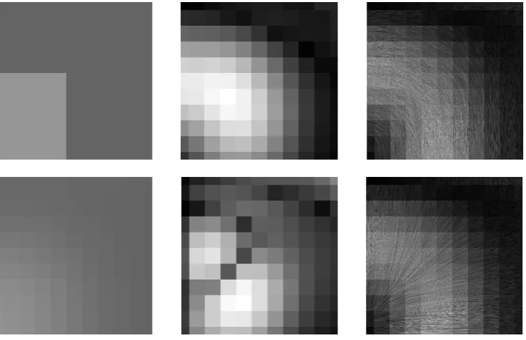
[ln(p),p∈P] ↑P ∗sn(x) ln(x)
Figure3: Mapping from the coefficients [ln(p), p∈P] to the interpolated imageln(x) of ordern, depicted as a two-stage process. The
standard notations∗and↑are used to denote the convolution and upsampling operations, respectively.
l(x)
∗aN(−x)
∗a2(−x)
∗a1(−x) ↓P
↓P
↓P
[lN(p),p∈P]
. . . [l2(p),p∈P]
[l1(p),p∈P] ↑P
↑P
↑P
∗sN(x)
∗s2(x)
∗s1(x)
+ l(x)
Figure4: Local signal analysis and synthesis, whereNdenotes the number of different templates (Nmay be infinite).
forn∈N, where
v2(x)=w2(x)
h2(x) =
w2(x)
p∈Pw2(x−p) (13)
is a modified window. This latter window has the property that the sum of displaced copiesv2(x−p) for all positions
pon the sampling latticeP is equal to one for all positions x∈F.
The resulting synthesis stageSis specified by
l(x)= p∈P
n∈N
ln(p)·sn(x−p)
= p∈P
n∈N ln(p)·an(x−p)
p∈Pw2(x−p) ,
(14)
forx∈F. This optimal synthesis corresponds tou(x)=w(x) in our earlier notation.
If an impulse signal with unit weight at positionpis input into a filter with impulse responsesn(x), then the output is, by definition, equal tosn(x−p). This implies that the signal
ln(x)=
p∈P
ln(p)·sn(x−p) (15)
is the output of this filter in case the input is an array of im-pulses, where the weight of the impulse at positionp ∈ P is equal to the coefficientln(p). This operation of creating an array of impulses from a set of coefficients is called upsam-pling. The combined operation of upsampling and filtering is calledinterpolationand is depicted inFigure 3. The com-plete signal synthesisS contains several of these interpola-tions, that is, one for each indexn∈N, and is hence a mul-tirate filter bank. The synthesized signal arises by combining all outputs of this multirate filter bank.
The overall image analysis and synthesis is depicted in Figure 4. In case ofFigure 4, the coefficients [ln(p)] that are derived from the original image are not modified, so that the
output signal satisfiesl(x)=l(x), forx∈F. IfFis discrete, then the local signal decomposition can be used to interpo-late the input signal, that is, to construct signal valuesl(x), for x ∈F[13]. In case of image processing or coding, the orig-inal coefficients are mapped to modified coefficients [ln(p)] before entering the synthesis stage [1], so thatl(x)=l(x), for x∈F.
Note that a local signal decomposition satisfies not only the global correspondence of (14), that is, synthesis after analysis results in the original signal, but also the local corre-spondences of (3). The latter correspondences imply that the local description [l]p=[ln(p), n∈N] completely specifies the signall(x) within the local windoww(x−p) at position p. The windowed signal
lw(x−p)=w2(x−p)·l(x)=
n∈N
ln(p)·an(x−p) (16)
also expresses the contribution of the coefficients [l]p =
[ln(p), n∈N] at positionp∈P to the overall synthesized signal, in a way that is specified in (14).
3. PARTIAL SIGNAL DECOMPOSITIONS
One obvious disadvantage of local signal decompositions is that a large number of filter operations (i.e., equal to the car-dinality of the index setN) may be required in the most gen-eral case in order to create the processed signal
l(x)= p∈P
n∈N
ln(p)·sn(x−p)
= p∈P
n∈Nln(p)·an(x−p)
p∈Pw2(x−p) .
(17)
The specific dependency of the output coefficients [l]p =
allow for substantial simplifications. We discuss an impor-tant special case.
We assume that the index set can be subdivided in two subsets, that is,N =No∪Nr, in such a way that the output coefficients [ln(p),n∈No] at positionponly depend on the corresponding input coefficients [ln(p), n ∈ No], and the remaining coefficients at positionpare all transformed in an identical way, that is,
ln(p)=κ(p)·ln(p), (18)
forn∈Nr. We moreover assume that the adaptive weight-ing factorκ(p) on the coefficients in the index setNrcan be derived from [ln(p), n∈No] and the local energy
E(p)=
Fw
2(x−p)·l2(x)dx. (19)
Because the local basis{ϕn(x−p), n∈N}was assumed to be orthonormal, this local energy can be split into
Eo(p)=
n∈No
ln(p)2
, (20)
the local energy in the signal component
n∈No
ln(p)·ϕn(x−p)w(x−p) (21)
described by the first index set No, and the residue energy
Er(p)=E(p)−Eo(p), that is, the local energy in theresidue
signal
n∈Nr
ln(p)·ϕn(x−p)w(x−p)
=
l(x)−
n∈No
ln(p)·ϕn(x−p)
w(x−p) (22)
that is described by the second index setNr.
Using the above assumptions, it is easily verified that the processed signal can be expressed as
l(x)=
p∈P
n∈No
ln(p)−κ(p)·ln(p)
·sn(x−p)+l(x)·κ(x).
(23)
This so-calledpartial signal decompositionleads to the mod-ified algorithm depicted inFigure 5. Only a partial transfor-mation involving the indicesn∈Nois hence required in this case to determine the processed signal. The missing informa-tion for the other indicesn∈Nr can be recovered from the original signal. The weighting function
κ(x)=
p∈P
κ(p)·v2(x−p) (24)
that must be applied to the original signal in order to accom-plish this correction is obtained by interpolating the adap-tive factors [κ(p), p∈P] with a filter with impulse response equal to the modified window functionv2(x). In case of
im-age coding, where the original signal is not available at the re-ceiver side, we obviously need to chooseκ(p)=0,∀p∈P. Nonzero values ofκ(p) are however useful in case of image processing.
4. RESIDUE-IMAGE PROCESSING
4.1. Algorithm
The simplest case of a partial signal decomposition arises when the index setNocontains only a single component, that is, the local average signal value
lo(p)=
Fw
2(x−p)·l(x)dx, (25)
and the residue signall(x)−lo(p) is the local deviation from this average value. If we assume that the window function is normalized, that is, ifFw2(x)dx=1, then this corresponds
to a single orthonormal basis vectorϕo(x)=1 in the index setNo. If we impose that the local average signal valuelo(p) is not altered by the processing, then the partial signal decom-position can be expressed as
l(x)=
p∈P
v2(x−p)·lo(p) +κ(p)·
l(x)−lo(p)
=
p∈P
v2(x−p)·1−κ(p)l
o(p) +l(x)·κ(x), (26)
whereκ(p) denotes the residue amplification factor at posi-tionp∈P, andκ(x) is the corresponding interpolated func-tion.
In uniform regions of the image, the residue energy
Er(p)=
Fw
2(x−p)·l(x)−l o(p)
2
dx
=
Fw
2(x−p)·l2(x)dx−l2 o(p)
(27)
will be small, while in transition regions (i.e., near edges) Er(p) will be large. This residue energy can hence be used as a control variable in an adaptive processing algorithm that requires different processing for uniform and transition re-gions. This residue energy can be derived quite efficiently, since it involves only two filter operations, one on the origi-nal sigorigi-nall(x), and one on the squared signall2(x).
Both noise reduction and contrast enhancement can be achieved using residue-image processing [15]. The relation-ship between the residue amplification factorκ(p) and the residue energyEr(p), orresidue amplitudeAr(p)=
Er(p), makes the adopted strategy explicit. Many different ap-proaches can be imagined, but we discuss only one possibil-ity.
l(x)
(·)2
∗w2(−x)
Ao
↓P
[ln(p)]n∈No
[κ(p),p∈P]
Cp,κ(p)
To(Cp)
↑P
[ln(p)]n∈No
∗v2(x)
So + l(x) ×
Figure5: Algorithmic structure for partial image decompositions. In the analysis stepAo, the input imagel(x) is transformed into a limited
set of coefficients. These coefficients [ln(p), n∈No] at a given positionpundergo the transformationTo(Cp)=To(Cp)−κ(p)·Io, where To(Cp) is the intended transformation andIodenotes the identity transformation. The control variablesCpat positionp, which are used to select the desired transformationTo(Cp) and the weighting factorκ(p) on the missing coefficients, can be derived from [ln(p), n∈No] and
the local energyE(p). The transformed coefficients [ln(p)=ln(p)−κ(p)·ln(p),n∈No], where [ln(p),n∈No] are the intended coefficients
for the processed imagel(x), are combined in the synthesis stepSoto obtain part of the output image. The missing part of the processed
image is extracted from the original imagel(x) by a weighting functionκ(x) that interpolates the factors [κ(p),p∈P] to all positionsx∈F.
function of the input amplitudeAr(p). Many functions sat-isfy this condition, and a simple example is
κAr(p)
·Ar(p)=s·Ar(p) + (1−s)·Av (28)
forAt ≤Ar(p)≤Av, where 0≤s≤1 denotes the slope of the input-output amplitude characteristic. In this case, the maximum value of the amplification factor is
κAt
=s+ (1−s)·Av
At
(29)
forAr(p)=At, and decreases to 1 forAr(p)=Av. Alterna-tive expressions forκ(Ar(p)) that avoid the discontinuity at
Ar(p)=Atmay also be considered.
InFigure 6, we illustrate residue-image processing on an 8-bit subtractive angiography image (values between 0 and 255). The threshold value At = 3 was derived from the residue amplitude histogram (i.e.,At = 2·Am, whereAm is the mode of the residue amplitude histogram, see next section), and the remaining parameters wereAv = 15 and
s=0.1. A separable binomial window function [2] of size 7 (i.e., with coefficientsw2=[1 6 15 20 15 6 1]/64 in one
dimension) was used as the window function.
4.2. Energy histograms and noise estimation
Since images usually contain noise, the residue energyEr(p) will not most often be exactly zero, not even for regions that we consider to be uniform. We hence have to decide on a threshold value Et = A2t for the residue energy mea-sureEr(p), below which image positions are classified as be-longing to uniform regions. As part of this process, we need to estimate noise characteristics. This noise estimation may also be interesting in its own right, for example, to objectively characterize the quality of the image acquisition [17,19,24]. It has been demonstrated [15, 24] that the first-order statistic, that is, the histogram or probability density function (PDF), ofEr(p), at least in uniform regions of the image, can
Figure 6: Residue-image processing applied to a subtractive an-giography image. The top row shows the images, while the bot-tom row shows the corresponding residue amplitudes (Ar). The left
and right columns correspond to the original and the processed image, respectively. The displayed residue amplitude images show log(1 +Ar) instead ofArin order to allow better discrimination.
be approximated by aχ2-distribution
PEr
= 1
Eo(q−1)!
Er
Eo q−1
exp
−Er
Eo
, (30)
with 2qdegrees of freedom. The corresponding PDF for the residue amplitude is
PAr)= 2 Ao(q−1)!
Ar
Ao 2q−1
exp
−
Ar
Ao 2
, (31)
12 10 8 6 4 2 0
Amplitude 0
500 1000 1500 2000 2500
Nu
m
b
er
Data
χ2
Figure7: The drawn curve shows the histogram of the residue am-plitude for the image and processing used inFigure 6. The dotted curve corresponds to optimal fitting of theχ2-distribution (q=3.83
andAo=0.71, resulting in a peak value atAm=1.49).
Am = Aoq−0.5, respectively. Energy or amplitude his-tograms for an actual image can be compared against the above theoretical PDFs in order to find the PDF parame-ters Eo (or Ao) and q. Actual images of course also con-tain nonuniform regions. The corresponding responses for these image features will influence the shape of the energy histogram, especially for large energy (or amplitude) values. This implies that only the part of the histogram at low energy (or amplitude) values should be used for noise estimation and curve fitting against the theoretical PDF [24], as shown inFigure 7.
A parametrized PDF such as theχ2-distribution can be
used to performK-means clustering on the residue tude or energy. For example, if the observed residue ampli-tude histogramh(Ar) can be approximated by a sum of two components, that is,
hAr
=Po·P
Ar
+hAr
−Po·P
Ar
, (32)
where P(Ar) satisfies (31) and is associated with uniform regions, then maximum a posteriori classification will clas-sify all positionspfor which the residue amplitude satisfies Ar(p)< At, with
Po·P
At
=hAt
−Po·P
At
, (33)
as belonging to uniform regions. This provides us with an automated means of selecting the thresholdAt.
5. THE HERMITE TRANSFORMATION
5.1. Definition
We will now apply the theory of local signal decompositions to the specific case of a two-dimensional Gaussian window
w(x,y;σ)= 1
σ√πexp
−x2+y2
2σ2
(34)
with standard deviation equal toσ. Note that this window function is both separable, that is, can be written as the prod-uct of two Gaussian functions inx- andy-directions, and cir-cularly symmetric, that is, its value only depends on the dis-tancer = x2+y2 from the origin. Especially the circular
symmetry will turn out to be essential for the discussion that follows.
We select the basis functions of the signal decomposi-tion (which were denoted byϕninSection 2) to be orthonor-mal polynomials for the Gaussian window [2]. Because this window is separable, these orthonormal polynomials are also separable, that is,
pn−m,m(x,y;σ)=gn−m
x σ
·gm
y σ
, (35)
with
gn(x)= 1
√
2nn!Hn(x), (36) where the standard notation is used to denote the Hermite polynomialHn(x) of ordern, forn=0, 1,. . . .For the discus-sion in this paper, we will especially need the polynomials up to degree 2, that is,
g0(x)=1, g1(x)= √
2x, g2(x)=
2x2−1 √
2 . (37)
The resulting image decomposition at the generic1lattice
po-sition (0, 0) satisfies
w(x,y;σ)
l(x,y)− ∞
n=0 n
m=0
ln−m,m·pn−m,m(x,y)
=0,
(38)
where equality means convergence in the mean-square sense. TheHermite coefficients[ln−m,m; n = 0,. . .,∞; m = 0,
. . .,n] are derived by filtering the spatial image representa-tion l(x,y) withderivative-of-Gaussian filters with impulse responses
dn−m,m(x,y;σ)
=gn−m
−x
σ
gm
− y
σ
·w2(x,y;σ)
= 1
2n(n−m)!m!
∂n
∂(x/σ)n−m∂(y/σ)mw
2(x,y;σ),
(39)
1In order to simplify the notation we discuss only the contribution at lattice
or filter kernelsdn−m,m(−x,−y;σ), and selecting the filtered outputs at the lattice positions. For the generic lattice posi-tion (0, 0) this results in
ln−m,m= +∞
−∞dx +∞
−∞d y l(x,y)·dn−m,m(−x,−y;σ). (40)
The fact that the filter functions in (39) can be expressed as derivatives of Gaussians is a consequence of a well-known property of Hermite polynomials, that is,
e−x2Hn(x)=(−1)n d n
dxne −x2
. (41)
This property implies that the Hermite coefficients them-selves can also be interpreted as partial derivatives
ln−m,m= 1
2n(n−m)!m!
∂n
∂(x/σ)n−m∂(y/σ)ml(x,y;σ)
x=y=0
(42)
to the smoothed image
l(x,y;σ)=l(x,y)w2(x,y;σ) (43)
that is obtained by applying a Gaussian filter w2(x,y;σ)
with standard deviation equal toσ/√2 to the original image l(x,y).
Note that the contribution at the generic lattice position (0, 0) to the overall synthesized image is
lw(x,y)=w2(x,y;σ)·l(x,y)
= ∞
n=0 n
m=0
ln−m,m·dn−m,m(−x,−y;σ),
(44)
while the local energy at this position is equal to
E=
w2(x,y)·l2(x,y)dx d y= ∞
n=0 n
m=0
l2n−m,m. (45)
The residue energyEr =E−l200or residue amplitudeAr =
Ercan again be used to differentiate between uniform and nonuniform regions in the image.
InFigure 8we show an artificial image containing sev-eral interesting features such as edges, lines, corners, T-junctions, X-T-junctions, circles, and noise. We will use this image throughout this paper to illustrate different alterna-tive forms of the Hermite transformation because it is much easier to judge the properties of the Hermite transformation on this image than on a natural image.
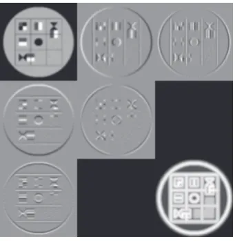
InFigure 9we show the residue amplitude and the Her-mite coefficients up to order 2 for a Gaussian window with spread σ = 2.5 times the sampling distance. The coeffi -cientsln−m,m for all positions are grouped into subimages. The (fuzzy) derivatives of ordern−malong thex-direction and order m along the y-direction are obtained by filter-ing the original image with the derivative-of-Gaussian filter dn−m,m(x,y) and (optionally) subsampling the filtered image. No subsampling has been applied in the case ofFigure 9. One important advantage of the derivative-of-Gaussian filters is that they are separable. This means that they can be imple-mented very efficiently by first filtering along thex-direction and subsequently along they-direction (or vice versa).
Figure8: Original image used in the Hermite analyses.
5.2. Scale space
Derivative-of-Gaussian filters play a key role in the theory of scale space [32,37,38]. Scale space represents a systematic way of studying structure in images. An image is regarded as a surface that can be analyzed at varying degrees of de-tail. To reduce the level of detail, the image is first passed through a Gaussian filter. The smoothed surface is then de-scribed using traditional methods from differential geometry (see alsoSection 7), a well-studied discipline of mathematics [39]. Many interesting surface properties can be expressed as combinations of the local partial derivatives ln−m,m of (42) to the smoothed imagel(x,y;σ). It is well known that this smoothed image is the solution to a diffusion equation
∂
∂tu(x,y,t)=
∂2
∂x2+
∂2
∂y2
u(x,y,t), (46)
with initial condition
u(x,y, 0)=l(x,y) (47)
that is stopped after time t = T = (σ/2)2. Fast recursive
methods for numerically solving this diffusion equation [40] may be used to determineu(x,y,T)=l(x,y; 2√T) for large values ofT. In the Hermite transformation the operations of smoothing and differentiating are combined, so that the Her-mite transformation corresponds to an analysis at a specified level in scale space.
Very often, the most efficient way for calculating the Her-mite coefficients is by combining diffusion and filtering, as shown inFigure 10. Indeed, if the input imagel(x,y) is first diffused up to timeT=(σD/2)2, and subsequently analyzed by a Hermite transformation with parameterσH, then the re-sulting coefficients at the origin, that is,
un−m,m=
dn−m,m(x,y;σH)u(x,y;T)
x=y=0= σ
H
σ
n
ln−m,m,
Figure9: Hermite coefficientsln−m,m, form=0,. . .,n, up to order n=2 for a Gaussian window with spreadσ =2.5 times the sam-pling distance. The image in the lower-right corner is the residue amplitudeAr. To relate the mathematical results in this paper to the
figures, it should be realized that thex-axis points to the right and they-axis downwards. Moreover, the coefficients of ordern, which are located in thenth diagonal, are amplified by the same factorβn
for display purposes. The factorsβnare chosen independently for
each ordern, in such a way that the complete display range is used.
u(x, y; 0)=l(x, y)
Diffuse for timeT
u(x, y;T) =l(x, y;σD)
Hermite (σH) un−m,m ·σ
σH n
ln−m,m
Figure10: The Hermite coefficients for a large standard deviation equal toσ can be obtained by a three-step process. First, a diff u-sion is applied to the original imageu(x,y; 0)=l(x,y) for a time
T, resulting in the diffused imageu(x,y;T) = l(x,y;σD), where σD =2
√
T. Second, a Hermite transformation with a small stan-dard deviation equal toσH, whereσH2 =σ2−σD2, is applied to the
diffused image, resulting in the coefficientsun−m,m, form=0,. . .,n
andn=0, 1, 2. . . .Third, these coefficients of ordernare rescaled by a factor (σ/σH)nto obtain the required Hermite coefficientsln−m,m.
belong to a Hermite transformation with parameter
σ=σD2+σH2 =
4T+σH2. (49)
An upper limit on σH allows to limit the size of the derivatives-of-Gaussian filters, since this filter size is pro-portional toσH. The number of computations required in the filtering stage increases (linearly) with this filter size. A lower limit on σH (typically, σH larger than 1.5 times the sampling distance [13]) is required to guarantee that the derivative operations can be closely approximated for digi-tal images. Most of the time we use a well-designed set of
derivatives-of-Gaussian filters (forσHequal to 1.8 times the sampling distance), and vary the diffusion timeTto accom-plish the required value ofσ.
5.3. Angular functions
An important step towards obtaining a better insight into the Hermite transformation is to express the filtering that is performed on the input image in the Fourier domain. The Fourier transformations of the filter functions, expressed in polar coordinates, are
Dn−m,m(ω,φ;σ)=Dn(ω;σ)·αn−m,m(φ), (50)
where
Dn(ω;σ)= 1
√
2nn!(−jωσ) nexp
−(ωσ)2
4
(51)
is the 1D Fourier transformation of thenth-order Gaussian derivative
Dn(r;σ)= 1
√
2nn!
dn
d(r/σ)n
1 σ√πexp
−r2
σ2
, (52)
and
αn−m,m(φ)=
n!
(n−m)!m!cos
n−mφ·sinmφ, (53)
form = 0,. . .,n, are theCartesian angular functionsof or-dern[2,20]. The shape of these Cartesian angular functions can be judged very well inFigure 9from the angular modu-lation of the coefficients along the edge of the circle image. The Cartesian angular functions of order n = 1 are sim-plyα10(φ)= cosφ andα01(φ)= sinφ, while the Cartesian
angular functions of ordern = 2, that is,α20(φ) = cos2φ,
α11(φ)= √
2 cosφsinφ, andα02(φ)=sin2φ, are plotted in
Figure 11.
The Hermite coefficients can be derived from the Fourier image representationl(ωx,ωy) through
ln−m,m= +∞
−∞
dωx 2π
+∞
−∞
dωy 2π l
ωx,ωy
·dn−m,m
ωx,ωy;σ
(54)
or, alternatively, by changing to polar coordinates, through
ln−m,m= 1 2π
2π
0 dφ
ln(φ)·αn−m,m(φ) (55)
form=0,. . .,n, where
ln(φ)= 1 2π
∞
0 ω dω
l(ω,φ)·Dn(ω;σ) (56)
3 2 1 0 −1 −2 −3 −1 −0.5 0 0.5 1
(2,0) (1,1) (0,2)
Figure11: Cartesian angular functions of ordern=2.
from the angular functionln(φ). One advantage of defining the “image” angular function as an intermediate step in the analysis is that it becomes straightforward to extend many of the results below, that is, those that only depend on the properties of the angular components of the filters, to filter banks in which the radial components of the filters, that is,
Dn(ω;σ), are not derivatives-of-Gaussians.
The Fourier transformation of the local imagelw(x,y)=
w2(x,y;σ)·l(x,y) can be expressed as
lw(ω,φ)=l(ω,φ)D0(ω)= ∞
n=0
Dn(ω)·ln(φ), (57)
where
ln(φ)= n
m=0
ln−m,m·αn−m,m(φ) (58)
is called the “derivative”angular functionof ordern. Since the interest here will be mainly in the derivative angular func-tions of ordern=1 andn=2, the following explicit expres-sions
l1(φ)=l10·cosφ+l01·sinφ,
l2(φ)=l20·cos2φ+l11· √
2 cosφsinφ+l02·sin2φ
(59)
are provided.
5.4. One-dimensional images
The Hermite coefficients at the generic lattice position (0, 0) describe the local imagelw(x,y) = w2(x,y;σ)·l(x,y). An important specific case of local patterns in 2D are 1D pat-terns, that is, patterns that vary only in one direction (and
are constant along the orthogonal direction). In natural im-ages, many of the image details that are of prime impor-tance, such as edges and lines, can be locally described as one-dimensional patterns, at least within the analysis win-doww(x,y;σ). Since analysis, coding, and processing of such patterns are considered important, it is worthwhile to inves-tigate them separately.
The angular function for a locally one-dimensional (1D) image with normal along direction (cosφo, sinφo), that is,
l(x,y)=l(xcosφo+ysinφo), has only contributions in the directionsφoandφo+πand is therefore of the form
ln(φ)=πln
δφ−φo
+ (−1)nδφ−φ o+π
, (60)
wherelnis thenth-order Hermite coefficient of the 1D signal
l(r).
For a 1D image we can express the Hermite coefficients as
ln−m,m=ln·αn−m,m
φo
, (61)
so that the “derivative” angular function becomes
ln(φ)=ln· n
m=0
αn−m,m
φo
·αn−m,m(φ)=ln·cosn
φ−φo
.
(62)
6. LOCAL COORDINATE AXES
6.1. Effect on Hermite coefficients
In scale-space theory [32], geometric features of the smoothed surfacel(x,y;σ) as a function of the position (x,y) (and scaleσ) are used for image analysis [41,42]. The well-established mathematical discipline of differential geometry [43] is especially concerned with how such geometric fea-tures can be derived, and some of the major results of ap-plying differential geometry for image feature extraction will be discussed inSection 7.
Adopting local coordinate axes
x
y
=
cosφo sinφo
−sinφo cosφo
·
x y
(63)
is one of the basic operations in differential geometry because many expressions for important surface properties can be simplified greatly in an adaptive coordinate system. For ex-ample, for the one-dimensional patterns introduced above, we will see shortly that aligning thex-axis with the direction of the pattern has distinct advantages.
We analyze the behavior of the angular functionsln(φ) andln(φ) under rotation of the coordinate axes. If we ro-tate the coordinate axes clockwise (or the image anticlock-wise) through an angleφo(in the left-handed coordinate sys-tem that is used in the figures), that is, if we changeln(φ) to
ln(φ+φo), then the Hermite coefficients in the local coordi-nate system (x,y) are equal to
ln−m,m
φo
= 1
2π
2π
0 dφ
ln(φ)·αn−m,m
φ−φo
for m = 0,. . .,n, and are related to the coefficients [ln−m,m, m=0,. . .,n] in the global coordinate system (x,y) by a linear transformation with parameterφo. The linear na-ture of the transformation is a consequence of the fact that both cos(φ−φo) and sin(φ−φo) can be expressed as linear combinations of cosφand sinφ. Specifically, since
αn,0
φ−φo
=cosnφ−φo
=
n
m=0
αn−m,m
φo
·αn−m,m(φ),
(65)
we obtain that the derivative of ordernalong directionφois given byln,0(φo)=ln(φo), which explains the name “deriva-tive” angular function for ln(φ). Based on then+ 1 partial derivatives [ln−m,m;m = 0,. . .,n], we can hence derive the directional derivativeln(φo) of ordernfor any directionφo [20,44]. The derivative angular function of orderncan of course also be expressed in terms of the Hermite coefficients in the rotated coordinate frame, that is,
ln(φ)= n
m=0
ln−m,m
φo
·αn−m,m
φ−φo
. (66)
Note that the linear transformation of the Hermite coef-ficients under rotation of the coordinate system requires that the image be locally approximated by a polynomial within a circularly symmetric windoww(x,y;σ). Rotating the coordi-nate axes can have a complicated effect on the Hermite coef-ficients, especially if the ordernis high. A systematic analysis for arbitrary orders has been performed [20], but is beyond the scope of this paper. In the remainder, we will only need the results for ordersn=1, that is,
l10 φo l01 φo =
cosφo sinφo
−sinφo cosφo · l10 l01 , (67)
andn=2, that is,
⎡ ⎢ ⎢ ⎣ l20 φo l11 φo l02 φo ⎤ ⎥ ⎥ ⎦=T2t·
⎡ ⎢ ⎣
cos2φo
0 sin2φo
0 1 0
−sin2φo
0 cos2φo
⎤ ⎥ ⎦·T2·
⎡ ⎢ ⎣ l20 l11 l02 ⎤ ⎥ ⎦, (68) where
T2= ⎡ ⎢ ⎢ ⎢ ⎢ ⎢ ⎣ 1 √
2 0 − 1 √ 2 1 √ 2 0 1 √ 2 0 1 0
⎤ ⎥ ⎥ ⎥ ⎥ ⎥ ⎦ (69)
is a unitary transformation matrix (with determinant equal to −1). These results for orders n = 1, 2 can also be ob-tained by straighforward manipulation of the goniometric
functions involved in (64), for example,
l1,0 φo = 1 2π 2π 0 dφ
ln(φ) cosφ−φo
= 1
2π
2π
0 dφ
ln(φ) cosφ·cosφo
+ 1 2π
2π
0 dφ
ln(φ) sinφ·sinφo
=l10·cosφo+l01·sinφo.
(70)
Since rotation of an image within a circularly symmet-ric window does not alter the signal energy contained in this window, we obtain that the local energy up to orderN satis-fies
EN= N
n=0 n
m=0
l2n−m,m= N
n=0 n
m=0
l2n−m,m
φo
, (71)
for allN ≥0. This also explains why the above transforma-tion matrices are unitary matrices.
6.2. Optimizing energy compaction
We now discuss how a suitable orientation for the local coor-dinate axes can be derived from the Hermite coefficients. For a 1D image with orientationφo, we obtain that
ln−m,m=ln·αn−m,m
φo
or ln−m,m
φo
=ln·αn−m,m(0), (72)
so thatln,0(φo) =ln(φo)= lnandln−m,m(φo)= 0, form = 1,. . .,n, in this case. We can hence split the local energy up to orderNas follows:
EN =l200+EN,1d
φo
+EN,2d
φo
=l2 00+
N
n=1
l2 n,0 φo + N
n=1 n
m=1
l2 n−m,m
φo
, (73)
whereEN,1d(φo) andEN,2d(φo) are the local 1D and 2D ener-gies up to orderNalong directionφo, respectively. We there-fore propose to use a strategy in whichφois selected such that
EN,1d(φo) is maximized.
InFigure 12, we show an adaptive Hermite transforma-tion of order N = 2 in which the local orientationφo has been selected by optimizingEN,1d(φo). Note the perfect en-ergy compaction that is obtained for 1D patterns. The 1D-amplitude AN,1d(φo) = [EN,1d(φo)]1/2 and 2D-amplitude
6.3. Gradient direction
In differential geometry, the reference angleφois often cho-sen such that the value of the derivative angular function of ordern=1, that is,
l1
φo
=l10·cosφo+l01·sinφo, (74)
is maximized. This is equivalent to optimizing the 1D en-ergy up to orderN =1. The above angular function can be rewritten as
l1
φo
=l1·cos
φo−φd
, (75)
withl1=
l102 +l201, provided that the angleφdsatisfies
tanφd=l01
l10
, (76)
or equivalently, l10 = l1·cosφd andl01 = l1 ·sinφd. The maximum value obviously occurs forφo=φd. This direction that makes an angleφd with the horizontal axis is called the
gradient direction.
In the neighbourhood of the generic lattice position (0, 0), the smoothed image can be expressed in both the global coordinate system (x,y) and the local coordinate sys-tem
xd
yd
=
cosφd sinφd
−sinφd cosφd
·
x y
, (77)
that is, l(x,y;σ) = ld(xd,yd;σ) are two equivalent descrip-tions of the same local image. The derivatives for a Cartesian coordinate system that is aligned with this gradient direction can hence be expressed as
ldn−m,m=
∂n
∂xn−m d ∂ydm
ld
xd,yd;σ xd=yd=0
=
2n(n−m)!m!
σn ln−m,m
φd
,
(78)
forn = 0, 1, 2,. . .andm =0,. . .,n. Selecting the reference angle along the gradient direction guarantees thatld
01 = 0.
The value
l10d = √
2 σ l1=
√
2 σ
l102 +l201 (79)
is called thegradient amplitude. The following explicit rela-tionships
ld 20=
2√2 σ2 l20
φd
, ld 11=
2 σ2l11
φd
, ld 02=
2√2 σ2 l02
φd
(80)
exist between the Hermite coefficients of order 2 and the second-order partial derivatives to the smoothed image ld(xd,yd;σ) for coordinate axes (xd,yd) oriented along the gradient direction.
Figure 12: Hermite coefficientsln−m,m(φo), form = 0,. . .,n, up
to ordern =2 for adaptive coordinate axes and a Gaussian win-dow with spreadσ =2.5 times the sampling distance. The image in the lower-right corner codes the local orientationφo. The image
at the right in the middle row is the 1D-amplitudeA2,1d(φo), while
the image at the bottom in the middle column is the 2D-amplitude
A2,2d(φo).
7. GEOMETRIC FEATURES
7.1. Planar curves
The geometric features that we will derive from the Hermite coefficients will all be characteristics of curves that are in some way defined by the surface functionl(x,y;σ). We will only consider curves that belong to a 2D plane, and there-fore start by summarizing some basic properties of such pla-nar curves. We denote byc(t)=(u(t),v(t)) the coordinates traced out by a curve segment in an orthogonal coordinate system (u,v) of a 2D plane (this plane need not be the im-age plane (x,y)). The parametertis defined for an interval of the real axis that includes 0, whilec(0) = (u(0),v(0)) is the point at which we want to measure the curve character-istics. We assume that the functionsu(t) andv(t) that relate the parametertto the curve coordinates are at least twice dif-ferentiable.
We will use two well-known properties of planar curves that are both illustrated inFigure 13. First, the tangent line to the curve at positionc(t) has the direction indicated by the tangent vector
ct(t)= 1
u(t)2+v(t)21/2
u(t),v(t). (81)
This vector can be used as the first vector in a right-handed orthonormal coordinate system. The second coordinate vec-tor thus defined is called the normal vectorand can be ex-pressed as follows:
cn(t)= 1
u(t)2+v(t)21/2
−v(t),u(t). (82)
v
u
cn(t)
c(t)
ct(t)
1
κ(t)·cn(t)
c(t) + 1
κ(t)·cn(t)
Figure13: The tangent vectorct(t) at the curvec(t) can be
com-bined with the normal vectorcn(t) to obtain a right-handed
or-thonormal coordinate system. The circle with radius 1/|κ(t)|has second-order contact with the curvec(t).
curves tells us how to measure this rate of change. More specifically, there exists a circle that is tangent to the curve atc(t) and for which the normal vector to the curve turns at the same rate as the normal vector to the circle when mov-ing in the direction of the tangent vector (i.e., this circle has second-order contact with the curve). This circle has radius 1/|κ(t)|and its center is located at position
c(t) + 1
κ(t)cn(t), (83)
where
κ(t)=u(t)·v(t)−u(t)·v(t)
u(t)2+v(t)23/2 (84)
is called thecurvatureat positionc(t) [43]. A positive or neg-ative curvature implies that the curve bends towards or away from the normal vector, respectively.
7.2. Isophote curvature
A first planar curve that can be derived from the surfacez=
ld(xd,yd;σ) is theisophotethrough the origin, defined by
ld
u(t),v(t);σ=ld
u(0),v(0);σ (85)
for some parameter interval includingt=0. This is the curve that arises if the image surface is intersected with a horizontal plane through the surface at the point of interest. The image value along the isophote does not change as a function oft,
so that
d dtld
u(t),v(t);σ
t=0=l d
10·u+l01d ·v,
d2
dt2ld
u(t),v(t);σ
t=0 =ld
20·(u)2+ 2l11d ·uv+l02d ·(v)2+ld10·u+ld01·v
(86)
are both equal to zero. Since the coordinate system is aligned along the gradient direction, that is,ld01 =0, we obtain that
u(0)=0 andu(0)= −[v(0)]2·ld
02/ld10, which in turn leads
to the expression
κi= − u (0)
v(0)2 =
ld 02
ld10
= 2
σ l02
φd
l10
φd
, (87)
for theisophote curvatureat the origin.
Since isophotes will have a high curvature near a corner, such as the one shown inFigure 14, the isophote curvature can assist in corner detection. More specifically, finding local maxima in the derivedisophote curvature measure
mi=κi·
ld10 31/3
=ld02·
ld10 21/3
, (88)
which also contains contrast information by including the image gradient ld10, is a frequently used method for
select-ing corner candidates.Figure 14illustrates that, although the position of a maximum in the isophote curvature measure is usually very close to the true corner position, both posi-tions will usually not coincide. This implies that a maximum in the isophote curvature measure can at best be used as an indication for the presence of a corner, and that a more in-depth analysis is required, for instance to update the position estimate of the corner feature [32].
The isophote curvature measure for the entire test image ofFigure 8is shown inFigure 15(a).
7.3. Flowline curvature
A second planar curve that can be derived from the surface z=ld(xd,yd;σ) is theflowlinethrough the origin, defined by the demand that the tangent to the flowline is equal to the image gradient, that is,
u(t)= ∂
∂xdld
xd,yd;σ
xd=u(t),yd=v(t) ,
v(t)= ∂
∂ydld
xd,yd;σ
xd=u(t),yd=v(t) ,
(89)
for some parameter interval includingt=0. Note that, at the origin, the flowline is orthogonal to the isophote.
Evaluating the second derivatives to the flowline at the origin results in
u(0)=ld20·u(0) +l11d ·v(0)=l20d ·ld10,
v(0)=ld11·u(0) +l02d ·v(0)=l11d ·ld10
![Figure 3: Mapping from the coestandard notationsfficients [ln(p), p ∈ P] to the interpolated image �ln(x) of order n, depicted as a two-stage process](https://thumb-us.123doks.com/thumbv2/123dok_us/1143236.1143443/4.600.166.437.157.270/figure-mapping-coestandard-notationscients-interpolated-order-depicted-process.webp)