R E S E A R C H
Open Access
Efficient and accurate image alignment using
TSK-type neuro-fuzzy network with
data-mining-based evolutionary learning algorithm
Chi-Yao Hsu, Yi-Chang Cheng and Sheng-Fuu Lin
*Abstract
Image alignment is considered a key problem in visual inspection applications. The main concerns for such tasks are fast image alignment with subpixel accuracy. About this, neural network-based approaches are very popular in visual inspection because of their high accuracy and efficiency of aligning images. However, such methods are difficult to identify the structure and parameters of neural network. In this study, a Takagi-Sugeno-Kang-type neuro-fuzzy network (NFN) with data-mining-based evolutionary learning algorithm (DMELA) is proposed. Compared with traditional learning algorithms, DMELA combines the self-organization algorithm (SOA), data-mining selection method (DMSM), and regularized least square (RLS) method to not only determine a suitable number of fuzzy rules, but also automatically tune the parameters of NFN. Experimental results are shown to demonstrate superior performance of the DMELA constructed image alignment system over other typical learning algorithms and existing alignment systems. Such system is useful to develop accurate and efficient image alignment systems.
Keywords:subpixel accuracy, TSK-type neuro-fuzzy network, data-mining based evolutionary learning algorithm, regularized least square
1. Introduction
Accurate and efficient image alignment is widely applied to many industrial applications, such as automatic visual inspection, factory automation, and robotic machine vision. Among them, visual inspection is usually required at finding a geometric transformation to align images. More specifically, the geometric transformation is commonly used as an affine transformation, which is consists of scaling, rotation, and translation, for aligning images. In other words, an affine transformation is con-sidered of great importance in designing image align-ment systems. Thus, it raises a challenge to provide an efficient affine transformation. To this end, neural net-work-based methods have widespread to address this challenge because such methods often feed global fea-tures of inspected images into a trained neural network to estimate affine transformation parameters [1-4]. In other words, neural networks are helpful for designing image alignment systems. Thus, there is a need to
develop a neural network-based image alignment system to demonstrate high performance [5]. To this end, the aim of this study is to design a learning algorithm to train a neural network that can estimate affine para-meters precisely.
Regarding the aim, this study adopts weighted gradi-ent origradi-entation histograms (WGOH) [6] as an image descriptor, which extracts the features from inspected images, to be the input of the neural network. Such representation technique has been proven a good descriptor in several literatures [7,8]. After that, we propose a novel learning algorithm to improve the robustness of neural networks. To be more specific, the proposed learning algorithm combines the self-organiza-tion algorithm (SOA), data-mining selecself-organiza-tion method (DMSM), and regularized least square (RLS) method to automatically identify the structure and parameters of the network. Once our learning method is applied, the structure of the network will be variable instead of a fixed one. Moreover, automatic tuning the parameters of the network can get more dynamic search space than a heuristic way. In other words, the structure and * Correspondence: [email protected]
Department of Electrical Engineering, National Chiao-Tung University, 1001 Ta Hsueh Road, Hsinchu 300, Taiwan
parameters of neural networks will become more robustness. The major contribution of this study is that the proposed learning method is helpful to develop effi-cient image alignment systems by automatically tuning the systems’structure and parameters.
The rest of this article is organized as follows. Section 2 gives a review of related studies. In Section 3, the pro-posed methodology for automatic aligning industrial images is introduced. The experimental results are pre-sented in Section 4. In Section 5, a conceptual frame-work for developing image alignment systems is described. The conclusion is attained in the last section.
2. Related studies
The problem of precisely aligning images has been well studied in several fields. For a broad introduction to image alignment methods, the related literature has been reviewed on several occasions [9,10]. To brief sur-vey, prior aligning methods can be classified as feature-and area-based methods [9,11]. Zitova feature-and Flusser [10] pointed out that area-based methods are preferably applied to the images which have not many details. Moreover, Amintoosi et al. [11] indicated that as the signal-to-noise ratio (SNR) is low, area-based methods produce better results than feature-based methods. In this study, we assume that our proposed image align-ment system is developed for industrial inspection tasks such that the captured images usually have less detail. Thus, area-based methods that adopt global descriptors are recommended in this article.
Recently, neural network-based image alignment uti-lizing global features has been a relatively new research subject. Such methods demonstrated high alignment speed since it only needs to feed the extracted feature vectors into the trained neural network to estimate the transformation parameters. For example, Ethanany et al. [1] presented a feedforward neural network (FNN) to align images through 144 discrete cosine transform (DCT) coefficients as the feature vectors. Their study showed that the FNN demonstrated high tolerance in deformed and noisy images. Moreover, based on FNN research, Wu and Xie [2] utilized low-order Zernike moments to replace DCT to further improve the perfor-mance of Ethanany’s study, which adopted larger dimen-sion of feature vector to represent an image sufficiently for the un-orthogonality of DCT-based space. As shown in their results, the proposed method can reduce the dimension of feature vector but their alignment results are not satisfied. More recently, Xu and Guo [3] adopted isometric mapping (ISOMAP) to reduce the dimension of feature vector. Their study demonstrated that ISOMAP can drastically reduce the dimension of feature vector to improve the computational efficiency. Nevertheless, the over fitting problem could happen in
FNN when a neural network is over learnt for training sets. Thus, the unseen pattern may be hard applied to this over-trained FNN since the network cannot provide the good ability of generalization. Owing to this pro-blem, Xu and Guo [12] used a Bayesian regularization method to improve the capability of generalizing the FNN. They showed some comparative experiments that FNN with regularization indeed performed better than without regularization.
Aforementioned studies indicated that the FNN is helpful to improve the alignment efficiency. However, such methods used steepest descent technique to mini-mize the error function such that it may reach the local minimal. In addition, it must take a large number of iterations to minimize the error function and several training attempts are needed to provide a robust FNN. In that respect, evolutionary algorithms appear to be better candidates than steepest descent method [13-15]. Because such learning methods are global and parallel search, they have more chance to converge toward glo-bal solution. Therefore, training a neural network utiliz-ing evolutionary algorithms has been an important field.
diversity, there is no systematic way to identify suitable groups for selecting chromosomes. Thus, it could result in slow rate of convergence.
To this end, this study proposes a TNFN with data-mining-based evolutionary learning algorithm (DMELA) to solve the abovementioned problems. In the first place, DMELA encodes an antecedent part of a TSK-type fuzzy rule into a chromosome and utilizes a RLS to estimate the consequent part of a TSK-type fuzzy rule. Such combination not only reduces the number of para-meters that must be trained, but also increases the con-vergence speed. Later, DMSM is used to explore the association rules that can identify suitable and unsuita-ble groups for chromosome selection. This action would solve the random group combination problem yielded by MGCSE. Finally, the SOA is utilized to decide suit-ability of different number of fuzzy rules. Thus, SOA is useful to automatic construct the structure of neuro-fuzzy networks (NFNs). In short, DMELA benefits both structure and parameters learning of a TNFN and it col-locates with WGOH descriptor to provide a framework to develop accurate and efficient image alignment systems.
3. Methodology
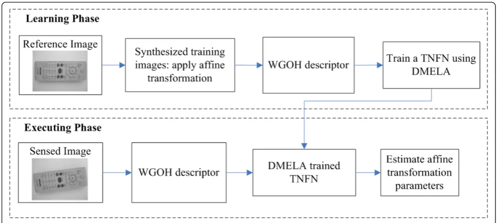
The flow chart of the proposed image alignment algo-rithm, which consists of learning and executing phase, is illustrated in Figure 1. During the learning phase, the synthesized training images are created by applying the reference image to affine transformations with randomly selected parameters, and then use the WGOH descrip-tor to represent these training images as feature vecdescrip-tors.
Finally, the feature vectors and desired targets are employed to train a TNFN using DMELA. During the executing phase, the sensed image is sent to the WGOH descriptor to extract a feature vector and then feed it into the DMELA-trained TNFN to estimate affine trans-formations parameters.
3.1. Synthesized training images
Image alignment can be viewed as a mapping between two images by means of a geometric transformation. Typically, affine transformation, which composites of translation, rotation, and scaling, is the most commonly used type. This article adopts the affine transformation as the transformation model and it can be described by the following matrix equations:
x2 y2
=s
cosθ −sinθ sinθ cosθ
x1−xc y1−yc
+
xc+x yc+y
,(1)
where (x1, y1) indicates the original image coordinate,
(x2,y2) indicates transformed image coordinate, s is a
scaling factor, (Δx, Δy) is a translation vector, θ is a rotation angle, and (xc, yc) is the center of rotation.
Thus, the synthesized training images can be generated by applying various combination of translation, rotation, and scaling transformations within a predefined range.
3.2. WGOH descriptor
The WGOH has been proven a good descriptor by a global feature selection approach (GFSA), which has been presented in our previous research [7]. Such descriptor was compared with other five global descrip-tors and results showed that WGOH demonstrated best
performance. Therefore, this article adopts WGOH as a descriptor to represent inspected images.
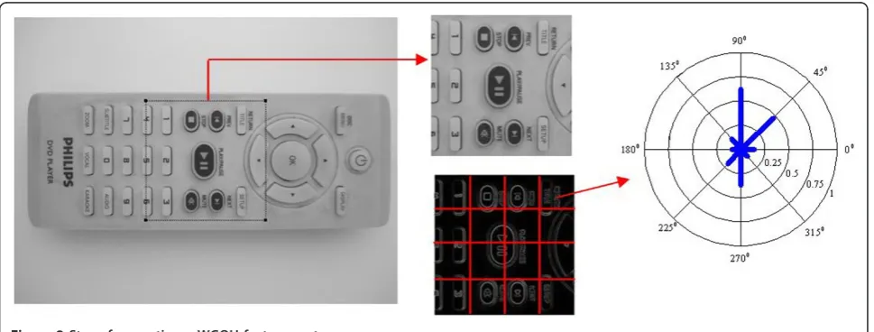
The WGOH descriptor was inspired by scale invariant feature transform (SIFT) descriptor [19], and presented by Bradley et al. [20] to show its high speed. The main idea of the WGOH is that it calculates the orientation histograms within a region, and uses the magnitude of the gradient at each pixel and the 2D Gaussian function to weight the histogram [6]. Therefore, for the WGOH descriptor, there are four steps for representing an image:
1. For each image, we capture the template window, whose location is at the center of the image, to be a place of extracting features. Within the window, we divide the length and width of the window into four equal parts to form 4 × 4 grids. Each grid is considered a sub-image. Thus, the template window can be split into 4 × 4 sub-images.
2. On each pixel of the sub-image (I(x,y)), the gradi-ent magnitudem(x, y), and orientationθ(x, y) are com-puted using pixel difference which the equations can be written as
m(x,y) =
(I(x+ 1,y)−I(x−1,y))2+ (I(x,y+ 1)−I(x,y−1))2, (2)
θ(x,y) = tan−1((I(x,y+ 1)−I(x,y−1))/(I(x+ 1,y)−I(x−1,y))). (3)
3. Calculate the 8-bin orientation histograms (each bin cover 45°) within each sub-image which are weighted by the gradient magnitude, and the Gaussian function.
4. Concatenate 8-bin histograms of 16 sub-images into a 128-element feature vector, and normalize it to a unit length. To reduce strong gradient magnitudes, the ele-ments of the feature vector are limited to 0.2, and this vector is normalized again.
Consequently, each image can be represented by a 128-elemet feature vector. Figure 2 illustrates an exam-ple of WGOH computation steps. Because the 128-ele-met feature vector is still too high to train a TNFN, there is a requirement of finding a dimensionality reduc-tion method to lower the dimension of the feature vec-tor. According to [21], genetic algorithm outperformed than principal component analysis and linear discrimi-nate analysis as dealing with their speaker recognition case. Thus, in our image alignment case, we adopted genetic algorithm method described in [22] to reduce a 128-elemet into a 33-element feature vector in the experimental section.
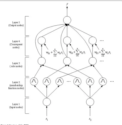
3.3. Structure of TNFN
In general, three typical types of NFN are the TSK-type, Mamdani-type, and singleton-type. According to [23,24], the authors have shown that a TNFN can offer better network size and learning accuracy than a Mamdani-type NFN. Thus, for our image alignment task, we only compare the TNFN with the singleton-type NFN in the experimental section to prove that the TNFN outper-forms the singleton-type NFN.
A TNFN [25] employs a linear combination of the crisp inputs as the consequent part of a fuzzy rule. The fuzzy rule of the TSK-type neuro-fuzzy system is shown in Equation 4, wherenand jrepresent the dimension of the input and the number of the fuzzy rules, respec-tively.
IFx1isA1j(m1j,s1j) andx2isA2j(m2j,s2j). . .andxnis Anj(mnj,snj) THENy=w0j+w1jx1+. . .+wnjxn(4)
The structure of a TNFN is shown in Figure 3, where nrepresents the dimension of the input. It is a five-layer network structure. In the TNFN, the firing strength of a fuzzy rule is calculated by performing the following
“AND”operation on the truth values of each variable to its corresponding fuzzy sets by:
u(3)ij =
n
i=1
exp
⎛ ⎜
⎝− u
(1) i −mij
2
σ2 ij
⎞ ⎟
⎠, (5)
where u(1)
i =xi and u (3)
ij are the outputs of first and
third layers;mij andsijare the center and the width of
the Gaussian membership function of the jth term of
the ith input variable xi, respectively. In this article, the
reason of adopting the Gaussian membership function is that it can be a universal approximator of any nonlinear functions on a compact set [23].
The output of the fuzzy system is computed by:
y=u(5)=
M j=1
u(4)j
M j=1
u(3)j
=
M j=1
u(3)j (w0j+ n i=1
wijxi)
M j=1
u(3)j
, (6)
whereu(5)is the output of fifth layer,wijis the
weight-ing value with ith dimension andjth rule node, andM is the number of a fuzzy rule. Here, the dimension of the output is set to be 4, and they are represented as a scaling factor (s), a rotation angle (θ), and translation parameters (Δx,Δy), respectively.
3.4. Data-mining-based evolutionary learning algorithm
The proposed DMELA aims to improve MGCSE [18]. Unlike MGCSE encoding one fuzzy rule into a chro-mosome, DMELA only encodes an antecedent part of a fuzzy rule into a chromosome. The consequent part of a fuzzy rule used in DMELA is estimated by an RLS approach. These two operations could not only reduce the number of parameters that must be trained, but also increase the convergence speed. Therefore, details of the coding step and RLS approach are described as follows:
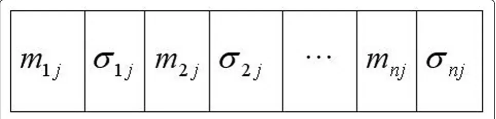
(1) Coding step
The coding structure of chromosomes in our proposed DMELA is shown in Figure 4. This figure describes an antecedent part of a fuzzy rule that has the form in Equation 4, where mij and sij represent a Gaussian
membership function with mean and deviation of ith dimension andjth rule node, respectively.
(2) RLS approach
Since the coding step only decides an antecedent part of a fuzzy rule, the consequent part is undetermined. In this article, RLS is adopted to estimate the consequent part. For simplicity, we only use two inputs (x1,x2) and
one output (y) to represent a two-rule TSK-type neuro-fuzzy system, which is described as follows:
Rule 1
IFx1isA11(m11,σ11) andx2isA21(m21,σ21), THENy1=w01+w11x1+w21x2, (7)
Rule 2
IFx1isA12(m12,σ12) andx2isA22(m22,σ22), THENy2=w02+w12x1+w22x2, (8)
whereAij andBij are the linguistic parts with respect
the inputi andRule j. From Equation 6, the output can be written as:
y= u1y1+u2y2
u1+u2 =u1y1ˆ +u2y2ˆ , (9)
whereu1andu2 are the firing strengths ofRules 1and
2, respectively, u1ˆ =u1/(u1+u2), and u2ˆ =u2/(u1+u2). Combine Equations 7-9, and we can get the following equation:
y=uˆ1y1+uˆ2y2=uˆ1(w01+w11x1+w21x2) +uˆ2(w02+w12x1+w22x2)
= (uˆ1x1)w11+ (uˆ1x2)w21+ˆu1w01+ (uˆ2x1)w12+ (uˆ2x2)w22+uˆ2w02. (10)
Since u1ˆ , u2ˆ , x1, and x2 are known values, the only
unknown value is the consequent part wij. Suppose a
given set of training inputs and desired outputs is
x(t),yd(t) M
t=1. Equation 10 can be rewritten as:
AW=Y, (11)
where
A= ⎡ ⎢ ⎢ ⎢ ⎣
ˆ
u1(1)x1(1) uˆ1(1)x2(1) uˆ1(1) ˆu2(1)x1(1) uˆ2(1)x2(1) ˆu2(1)
ˆ
u1(2)x1(2) uˆ1(2)x2(2) uˆ1(2) ˆu2(2)x1(2) uˆ2(2)x2(2) ˆu2(2)
..
. ...
ˆ
u1(M)x1(M)uˆ1(M)x2(M)ˆu1(M)ˆu2(M)x1(M)uˆ2(M)x2(M)uˆ2(M)
⎤ ⎥ ⎥ ⎥
⎦, (12)
and
W=w11w21w01w12w22w02
. (13)
In general, there is no exact solution to solve for W. Instead, a least square method is utilized to obtain an approximate solution. Moreover, to get the smooth esti-mation, the regularization is adopted. To this end, such method is named as RLS approach. Using RLS, the approximation solution is as follows:
ˆ
W= (ATA+λI)−1ATY, (14)
where l is a regularization parameter which adjusts the smoothness. Therefore, by getting Equation 14, we
complete the estimation the consequent part of fuzzy rules. Such operation can easily be expanded toninput, m output, andr fuzzy rules of a TNFN. To compare with MGCSE, the consequent part used in this article is computed by an RLS approach rather than tuned by an evolutionary procedure. Such action would increase the convergence speed because RLS approach directly calcu-lates the consequent part one time to minimize the errors between real and desire outputs. Nevertheless, evolutionary method tunes the consequent part many times to gradually minimize the errors.
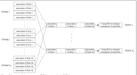
In addition to the above two processes, to consider the structure of TNFN, DMELA adopts the variable length of a combination of chromosomes with RLS method to construct a TNFN. To deal with this, multi-groups sym-biotic evolution (MGSE) is utilized in this article. Unlike the traditional symbiotic evolutions (TSEs) [17], each population in MGSE is divided into several groups, and each group represents a set of chromosomes that belongs to an antecedent part of one fuzzy rule. The structure of chromosomes to construct TNFNs in DMELA is shown in Figure 5. As shown in the figure, each antecedent part of a fuzzy rule represents a chro-mosome selected from a group,Psize denotes that there
are Psize groups in a population, andMk means that
there are Mk rules used in TNFN construction. Such
construction allows variable number of rules in TNFN. The learning process of DMELA in each group involves seven major operators: initialization, SOA,
DMSM, fitness assignment, reproduction strategy, cross-over strategy, and mutation strategy. This process stops as the number of generations or the fitness value reaches a predetermined condition. The whole learning process is described below:
3.4.1. Initialization
Before we start to design DMELA, the initial groups of individuals should be generated. The initial groups of DMELA are generated randomly within a fixed range. The following formulations show how to generate the initial chromosomes in each group:
Deviation:Chrg, c[p] =random[smin,smax],
wherep= 2, 4,. . ., 2n;g= 1, 2,. . .,Psize;c= 1, 2,. . .,NC, (15)
Mean:Chrg, c[p]= random[mmin,mmax],
wherep= 1, 3,. . ., 2n−1, (16)
where Chrg, c represents cth chromosome in thegth
group,NC is the total number of chromosomes in each
group,prepresents thepth gene in aChrg, c, and [smin, smax], [mmin, mmax] represent the predefined range to
generate the chromosomes. 3.4.2. Self-organization algorithm
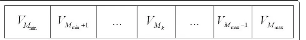
To select fuzzy rules automatically, SOA utilized the building blocks (BBs) to present the suitability of TNFN with different fuzzy rules. In Figure 6, SOA encodes the probability vector VMk, which stands for the suitability
of a TNFN with Mk rules, into BBs. In addition, in
SOA, the minimum and maximum number of rules must be predefined to limit the number of fuzzy rules to a certain bound, i.e., [Mmin,Mmax].
After BBs is defined, we use SOA to determine the suitable selection times of each number of fuzzy rules. The “selection times” indicates how many TNFNs should be produced in one generation. In other words, SOA is used to determine the number of TNFN with Mkrules in every generation. After the SOA is carried
out, the selection times of the suitable number of fuzzy rules in a TNFN will increase; otherwise, the selection times of the unsuitable ones in a TNFS will decrease. The processing steps of the SOA are described as follows:
Step 0. Initialize the probability vectors of the BBs:
VMk = 0.5, forMk=Mmin,Mmin +1, ...,Mmax; (17)
and
Accumulator = 0. (18)
Step 1. Update the probability vectors of the BBs according to the following equations:
VMk=VMk+ (Upt valueMk∗λ), if Avg≤fitMk
VMk=VMk−(Upt valueMk∗λ), otherwise
. (19)
Avg=
Mmax
Mk=Mmin
fitMk/(Mmax−Mmin); (20)
Upt valueMk =fitMk
Mmax
Mk=Mmin
fitMk; (21)
ifFitnessMk≥(Best FitnessMk−ThreadFitnessvalue)
thenfitMk =fitMk+FitnessMk,
(22)
where VMk is the probability vector in the BBs, lis a
predefined threshold value,Avg represents the average fitness value in the whole population, Best FitnessMk
represents the best fitness value of TNFN withMkrules,
and fitMk is the sum of the fitness values of the TNFN
withMkrules. In Equation 19, the conditions“fitMk ≥or
<Avg“ would affect the suitability of TNFNs with Mk
rules to be increased or decreased.
Step 2. Determine the selection times of TNFNs with different rules according to the probability vectors of the BBs as follows:
RpMk= (Selection Times)∗(VMk/Total Velocy), forMk=Mmin,Mmin +1,· · ·,Mmax, (23)
Total Velocy=
Mmax
Mk=Mmin
VMk, (24)
where Selection_Timesrepresents the total selection times in each generation and RpMk represents the
selec-tion times of TNFNs withMkrules in one generation.
Step 3. In SOA, to prevent suitable selection times from falling into the local optimal solution, we use two different actions to update VMk. Such actions are
defined in the following equations:
if Accumulator≤SOATimes, then do Steps 1 to 3, (25)
if Best Fitnessg=Best Fitness, then Accumulator=Accumulator+ 1, (26)
if Accumulator>SOATimes, then do Step 0 and Accumulator= 0, (27)
where SOATimesis a predefined value, Best_Fitnessg
represents the best fitness value of the best combination of chromosomes in the gth generation, andBest_Fitness represents the best fitness value of the best combination of chromosomes in the current generations. If Equation 27 is satisfied, then it indicates that the suitable selec-tion times may fall into the local optimal soluselec-tion. At this time, the processing step of SOA should return to Step 0 to initialize the BBs.
3.4.3. The DMSM
After the selection times are determined, DMELA further performs the selection step, which includes the selection of groups and chromosomes. In selection of groups, this article proposes DMSM to determine the suitable groups for chromosomes selection. To prevent the selected groups from falling into the local optimal solution, DMSM uses normal and explore actions to select well-performed groups. The details of the DMSM are discussed below:
Step 0. The transactions are built, as in the following equations:
if FitnessMk≥(Best FitnessMk−ThreadFitnessvalue)
Transactionj[i] =TFCRuleSetMk[i] then
Performance Index=g,
(28)
if FitnessMk<(Best FitnessMk−ThreadFitnessvalue)
Transactionj[i] =TFCRuleSetMk[i] then
Performance Index=b,
(29)
wherei= 1, 2,..., Mk, Mk=Mmin,Mmin+1,..., Mmax,j=
1, 2,...,TransactionNum, the FitnessMk represents the
fit-ness value of TNFN with Mk rules,ThreadFitnessvalue
is a predefined value,TransactionNum is the total num-ber of transactions, Transactionj[i] represents theith
item in the jth transaction, TFCRuleSetMk[i] represents
theith group in theMkgroups used for chromosomes
selection, andPerformance Index =g andPerformance Index =b represent the good and bad performances, respectively. Hence, transactions have the form shown in Table 1. As shown in Table 1, the first transaction means that the three-rule TNFN formed by the first, fourth, and eighth groups have“good”performance. In contrast, the second transaction indicates that the four-rule TNFN formed by the second, fourth, seventh, and the tenth groups have“bad” performance.
Step 1. Normal action:
The aims of this action include two parts: accumulate the transaction set and select groups. Regarding the first part, if the groups fit Equations 28 and 29, then the groups are stored in a transaction. Regarding the second part, DMSM selects groups using the following equation:
if Accumulator≤NormalTimes
then GroupIndex[i] =Random[1,PSize],
(30)
where i = 1, 2,..., Mk, Mk = Mmin, Mmin+1,..., Mmax,
Accumulatardefined in Equation 30 are used to deter-mine which action should be adopted, GroupIndex[i] represents the selectedith group of the Mkgroups, and
Psize indicates that there arePsize groups in a population
in DMELA. If the best fitness value does not improve
for a sufficient number of generations (NormalTimes), then DMSM selects groups according to explore action.
Step 2. Explore action:
If Accumulator exceeds theNormalTimes, then the current action switches to the explore action. The objec-tive of this action is to adopt the notion of DMSM to explore suitable groups in transactions. The major operations of DMSM include FP-growth performing, association rules generating, and suitable groups select-ing. The details of these three operations are presented below.
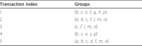
i. FP-growth performing In this operation, only good groups, whose performance index showed “g“ in Table 1, are performed with FP-growth and bad groups are skipped. Thus, frequently occurring groups can be found according to the predefined Minimum_Support, which stands for the minimum fraction of transactions containing the item set. After Minimum_Support is defined, data mining using FP-growth is performed. The FP-growth algorithm can be divided into two parts: FP-tree construction and FP-growth. The sample transactions are shown in Table 2. In this example, Minimum_Support= 3.
(1) FP-tree Construction
To construct a FP-tree, we first scan the transactions and retrieve the frequent 1-groupset which represents the set with bigger support counts than Minimum_ Support in transactions. Then, the retrieved frequently occurring groups are arranged in descending order based on their supports. After that, we discard the infre-quently occurring groups and sort the remaining groups. Then, the result is shown in Table 3. Thus, the ordered transactions appeared in this table are utilized to construct a FP-tree.
Table 1 Transactions in the DMSM
Transaction index Groups Performance index
1 1,4,8 g
2 2,4,7,10 b
... ... ...
TransactionNum 1,3,4,6,8,9 g
Table 2 Sample transactions
Transaction index Groups
1 {b, c, e, f, g, h, p}
2 {a, b, c, f, i, m, o}
3 {c, f, i, m, o}
4 {b, c, e, s, p}
5 {a, b, c, d, f, m, o}
Table 3 Transactions after discarding the infrequent groups and sorting the remaining groups
Transaction index Groups Ordered groups
1 {b, c, e, f, g, h, p} {c, b, f} 2 {a, b, c, f, i, m, o} {c, b, f, m, o} 3 {c, f, i, m, o} {c, f, m, o}
4 {b, c, e, s, p} {c, b}
The steps in FP-tree construction are illustrated in Figure 7a. In this figure (formed by scanning the last transaction in Table 3), the rightmost chart is called a prefix-tree of the frequent 1-groupset. Each node of the prefix-tree is composed of one group, a count of the fre-quent 1-groupset, and a node frefre-quently occurring group link. Afterward, the completed FP-tree shown in Figure 7b is created by combining the prefix-tree of the 1-groupset and the header-table.
(2) FP-growth
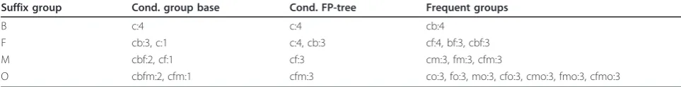
The FP-growth operation can be done by following steps: First, we choose each frequent 1-groupset as a suffix group, and find the corresponding set of paths connecting to the root of the FP-tree. The set of prefix paths is called the conditional group base. Second, we accumulate the count of each group in the base to construct the conditional FP-tree of the corresponding suffix group. Third, after exploring the frequently occur-ring groups in the conditional FP-tree, FP-growth data mining is completed by the concatenation of the suffix group with the generated frequently occurring groups. Finally, the frequent groups generated by the FP-growth are shown in Table 4.
ii. Association rules generating Once the frequently occurring groups are found, we can produce association rules from these frequent ones. For the purpose of iden-tifying the association rules with good performance, the frequent groups must combine the groups owing bad
performance shown in Table 1 to count the confidence degree. The confidence degree can be computed by the following formula:
confidence(frequent groups⇒good)
=P(good|frequent groups)
= supp(frequent groups∪good)
supp(frequent groups∪good) +supp(frequent groups∪bad),
(31)
where P(good|frequent groups) is the conditional probability, frequent groups ∪ good orbad means the union of frequent groups and good or bad performance, andsupp(frequent groups ∪ goodor bad) stands for the counts offrequent groupswith good or bad performance occurring in transactions. Then the rule is valid if
confidence(frequent groups⇒good)≥minconf, (32)
where minconfrepresents the minimal confidence given by user or expert. Hence, we can infer that if a rule satisfies Equation 32, then the frequent groups can be viewed as the suitable groups, otherwise they would be unsuitable groups. For instance, if the confidence of {1,3,6} ≥ {g} is bigger than the minimum confidence, then we construct this association rule. This rule indicates that the combination of the first, third, and sixth groups results in“good” performance. After doing so, the frequent groups are conduct to the association rules and generate theAssociatedGoodPool which con-tains all frequent groups satisfied Equation 32.
Figure 7Example of FP-tree construction.(a)Steps for constructing the FP-tree of sample transactions.(b)FP-tree of Table 5.
Table 4 Frequently occurring groups generated by FP-growth data mining
Suffix group Cond. group base Cond. FP-tree Frequent groups
B c:4 c:4 cb:4
F cb:3, c:1 c:4, cb:3 cf:4, bf:3, cbf:3
M cbf:2, cf:1 cf:3 cm:3, fm:3, cfm:3
iii. Suitable groups selecting After the association rules are identified, DMSM selects groups according to the association rules. The group indexes are selected from the associated good groups as the following equations:
if NormalTimes<Accumulator≤ExploreTimes
then GroupIndex[i] =w,
where w=GoodItemSet[q] =Random[AssociatedGoodPool],
(33)
where q= 1, 2,...,AssociatedGoodPoolNum i = 1, 2,..., Mk, Mk =Mmin, Mmin+1,...,Mmax, ExploreTimesare the
predefined value that judges to perform the exploring action,AssociatedGoodPool represents the sets of good item set that obtain from association rules, Associated-GoodPoolNum presents the total number of sets in AssociatedGoodPoolNumandGoodItemSet[i] presents a good item set that select from AssociatedGoodPool ran-domly. In Equation 33, if Mk greater than the size of
GoodItemSet, then remaining groups are selected by Equation 30.
Step 3. If the best fitness value does not improve for a sufficient number of generations (ExploreTimes), then DMSM selects groups based on the normal action.
Step 4. After the Mkgroups are selected, Mk
chromo-somes are selected fromMkgroups as follows:
ChromosomeIndex[i] =q, (34)
where q=Random[1,Nc], i= 1, 2,...,k,Nc represents
the total number of chromosomes in each group, and ChromosomeIndec[i] represents the index of a chromo-some that is selected from theith group.
3.4.4. Fitness assignment
In this step, the fitness value of an antecedent part of a fuzzy rule (an individual) is calculated by summing up the fitness values of all possible combinations in the chromosomes that are selected fromMkgroups that are
decided by DMSM. The steps in the fitness value assign-ment are described below:
Step 1. ChooseMkantecedent part of fuzzy rules with
RLS method to construct a TNFN RpMk times fromMk
groups with size NC. TheMkgroups are obtained from
the DMSM.
Step 2. Evaluate every TNFN that is generated from Step 1 to obtain a fitness value.
Step 3. Divide the fitness value byMkand accumulate
the divided fitness value to the selected antecedent part of fuzzy rules with their fitness value records that were set to zero initially.
Step 4. Divide the accumulated fitness value of each chromosome fromMk groups by the number of times
that it has been selected. The average fitness value represents the performance of an antecedent part of a
fuzzy rule. In this article, the fitness value is designed according the follow formulation:
Fitness Value = 1/(1 +E(y,y¯)), (35)
where
E(y,y) =
N
i=1
(yi−yi)2, (36)
where yi and ¯yirepresent the desired and predicted
values of the ith output, respectively, E(y,y) is a error function, and Nrepresents the number of the training data in each generation.
3.4.5. Reproduction strategy
Reproduction is a procedure of copying individuals according to their fitness value. This study adopted our previous research-elite-based reproduction strat-egy (ERS) [18] to perform reproduction. In ERS, every chromosome in the best combination of Mk
groups must be kept by performing reproduction step. In the remaining chromosomes in each group, this study uses the roulette-wheel selection method [26] for this reproduction process. The well-per-formed chromosomes in the top half of each group [27] proceed to the next generation. The other half is created by executing crossover and mutation opera-tions on chromosomes in the top half of the parent individuals.
3.4.6. Crossover strategy
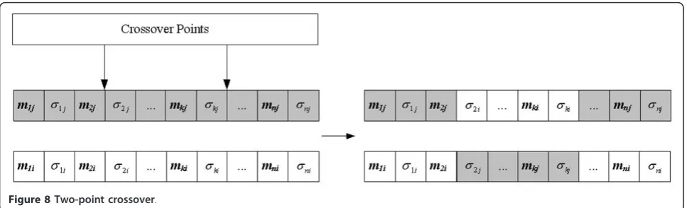
Although the reproduction operation can preserve the best existing individuals, it does not create any new individuals. In nature, an offspring can inherit genes from two parents. The major way to the inheritance of parents is the crossover operator, the operation of which occurs for a selected pair with a crossover rate. In this article, a two-point crossover strategy [26] is adopted and such strategy is illustrated in Figure 8. From this figure, exchanging the site’s values between the selected sites of individual parents creates new indi-viduals. The benefit of the two-point crossover is its ability of introducing a higher degree of randomness into the selection of genetic material [28].
3.4.7. Mutation strategy
3.5. Termination criterion
If the learning steps meet one of the following condi-tions, DMELA is terminated, and output the final results.
(1) The number of generations reaches a predefined maximal iteration value.
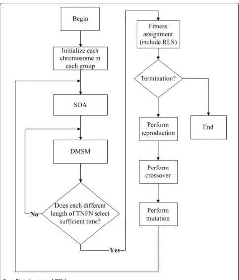
(2) Fitness value is greater than a fitness threshold. Consequently, the whole learning process of DMELA is summarized in Figure 9.
3.6. Time complexity analysis
In this section, to analyze the complexity of the pro-posed algorithm, we divide our method into six stages (skip the initialization stage) to discuss the complexity individually. Suppose the size of population is Psize, the
size of sub-population is Nc, the number of fuzzy rules
isM, the number of constructing fuzzy systems in one generation is S (i.e., the Selection_Times defined in Equation 23), the number of the training data isN, and the input dimension of NFN isn. The discussion of the complexity for each stage is as follows:
(1) SOA: in this stage, the only computation is to update the probability vectors (Equation 19) Stimes in one generation. Therefore, the complexity of SOA is O(S).
(2) DMSM: The DMSM operation includes normal and explore actions. In the normal action, since this action would be performed NormalTimes(appeared in Equation 30) in the overall learning process, the com-plexity of this action isO(NormalTimes). In the explore action, because the FP-growth and association rules mining are performed only in the beginning of this action or when the system falls into local optima. As a result, the effect caused by these two operations on the overall learning efficiency is not crucial. The complexity of these two operators can be skipped. Moreover, since the explore action would be performed (ExploreTimes -NormalTimes) times in the overall learning process, the
complexity of this action is O(ExploreTimes- Normal-Times), whereExploreTimesappeared in Equation 33.
(3) Fitness assignment: according to Equations 6 and 36, the evaluation of fitness one time requires NMn computations. Furthermore, there areSevaluation times in one generation. Thus, the complexity of fitness assignment is O(SNMn).
(4) Reproduction: in this stage, the roulette-wheel selection method is chosen to perform reproduction. Since each selection requiresNc steps and Nc spins to
fill the sub-populations [30], the total computation for a whole population in a generation is Nc2Psize. Therefore,
the complexity of reproduction stage is O(Nc2Psize).
(5) Crossover: to consider the selection of parents, the tournament selection is adopted to select parents. Since the tournament selection can be performed in constant time andNc PSizecompetitions are required to fill one
generation [30], the complexity of the tournament selection is O(Nc PSize). Moreover, the computation of
two-point crossover is constant in one generation. Thus, the complexity of crossover stage isO(NcPSize).
(6) Mutation: because the uniform mutation is adopted and the mutated gene is picked randomly from the chromosome, the mutation operator needsNc PSize
steps to fill overall populations. Hence, the complexity of mutation step isO(Nc PSize).
In summary, the dominate complexity of the proposed algorithm is the stage of fitness assignment (O(SNMn))). It indicates that the fitness assignment step would occupy most of the learning time.
3.7. Executing procedure
After training a TNFN, the executing phase of the proposed image alignment system merely consists of com-puting the WGOH descriptor and then feeding it into the DMELA-trained TNFN to get a scaling factors, a rotation angleθ, and translation parameters (Δx,Δy). About this, the proposed system is simple and efficient.
4. Experimental results
In the following experiments, visual inspection images, which are 640 × 480 pixels size, are used to examine the utility of the proposed image alignment method. Figure 10 depicts an example about such images where the left side is a reference image and the other side is a trans-formed image by a scaling, rotation and translation. Also in this figure, the dashed window represents a tem-plate window (the size is 200 × 200, and feature vectors are extracted within this window), and the cross sign denotes the reference location of the template.
In Table 5, four types of experimental images are pre-pared for simulation. The first three types of images are the synthesized ones generated randomly within the range in Table 6. In the last type of images are real ones captured from a camera. Moreover, Table 6 indicates the searching range for image alignment. If the affine transformation exceeds the range, then the image align-ment system may not promise high accuracy. Thus, the range of the image alignment defined in this article is restricted in Table 6.
All the experiments are performed using an Intel Core i7 860 chip with a 2.8 GHz CPU, a 3G memory, and the Matlab 7.5 simulation software.
The experimental results in this section contain four sections. Section 4.1 performs the comparison with
different types of NFNs. Comparison with existing learn-ing methods is presented in Section 4.2. In Section 4.3, synthesized images are used to compare the proposed image alignment system with other systems. Section 4.5 uses real images to validate the alignment accuracy of the proposed system.
4.1. Comparison with different types of NFN
In this section, we perform the comparison of a TSK-type and a singleton-TSK-type NFN. To setup an experiment, we run both types of NFN with the same number of fuzzy rules and the same population size described in Table 7 for 100 generations learning. Then such experi-ment is repeated 15 times using different initial condi-tions and final results are shown in Table 8. From this Figure 10Example of visual inspection images.(a)Reference image.(b)Testing image with scale = 0.9, rotation = -10°, vertical translation = 5, horizontal translation = 10.
Table 5 Experimental images preparation
Image type Image preparation
Synthesized images
600 images are generated with randomly selected affine parameters within the range described in Table 2
Training images
The 70% (420) of synthesized images
Testing images The 30% (180) of synthesized images
Real images Images are acquired from CCD camera with different pose from the reference image
Table 6 The range of affine transformation parameters used in experiments
Affine transformation parameter
The range of affine transformation parameter
Scale [0.7 1.3]
Rotation (degrees) [-30 30] Vertical translation (pixels) [-20 20] Horizontal translation (pixels) [-20 20]
Table 7 The initial parameters before training
Parameters Value Parameters Value
Psize 40 [Mmin,Mmax] [18, 25] Nc 20 [mmin,mmax] [-10, 10] Selection_Times 50 [smin,smax] [3, 15] NormalTimes 10 [wmin,wmax] RLS determined SearchingTimes 15 Minimum_Support TransactionNum/3 Crossover rate 0.6 Minimum_Confidence 60%
table, the TSK-type NFN exhibits lower image alignment error than the singleton-type NFN. Thus, we can con-clude that the TNFN would be performed better than the singleton-type NFN in our image alignment case.
4.2. Comparison with existing learning methods
Two typical evolutionary learning methods TSE [17] and MGCSE [18] are implemented carefully to compare with the proposed DMELA. To explore the number of fuzzy rules for TSE and MGSE, the fuzzy rules are tuned by setting the range of 20-100 in increments of 5. Thus, the results find that 85 and 80 rules are suitable for TSE and MGCSE, respectively.
In this simulation, training and testing images are ran-domly generated by the way specified in Table 5. Then 33-element feature vectors are obtained by applying WGOH with genetic algorithm-based dimensionality reduction described in [22] to above-generated images.
Moreover, before training, the initial parameters of DMELA are given in Table 7.
To consider SOA in DMELA, Figure 11 shows the results of the average probability vectors for 15 runs in different training and testing images. In this figure, the optimal number of fuzzy rules is 24. It represents that in most cases a 24-rule TNFN would have better perfor-mance than other rules within [Mmin, Mmax] = [18, 25].
Figure 12a-b depicts the learning curves and root mean square error (RMSE) of three different methods. From this figure, DMELA demonstrates fast conver-gence speed and less RMSE than TSE and MGCSE. In addition, due to RLS method utilized, the high initial fit-ness value would occur in Figure 12a.
Furthermore, to discuss the learning time, we add the time measurement on the proposed algorithm and per-form comparison with MGCSE and TSE. The running time defined in this article is to measure the time as the
Table 8 The comparison of the TNFN and the singleton-type NFN
Method Errors
ErrScale ErrAngle (degrees) ErrDx (pixels) ErrDy (pixels)
Mean SD Mean SD Mean SD Mean SD
TNFN 0.0054 0.0051 0.2106 0.1856 0.4702 0.3578 0.4326 0.4015
Singleton-type NFN 0.027 0.021 1.237 1.075 1.338 1.016 1.571 1.319
fitness of the algorithm reaches the predefined value. Thus, the results of three algorithms over 15 runs at dif-ferent initial conditions are reported in Table 9. As shown in this table, the proposed algorithm (DMELA) is much faster than MGCSE and TSE.
4.3. Comparison with existing image alignment systems
To evaluate the proposed system in comparison with other existing systems [3,12,19], the implementation of these existing systems are carefully cited in their original article. The comparison in this section consists of the alignment accuracy and robustness. These comparisons are discussed in the following parts.
4.3.1 Alignment accuracy
To compare the alignment accuracy of different systems, the training images, which are used to train neural net-works, and the testing images, which are used to check the alignment accuracy, are generated by the way described in Table 5.
Figure 13 depicts an alignment example for a testing image on three different systems. The cross sign in this figure denotes the estimated results. From this figure, the proposed system can estimate more accurate posi-tion and orientaposi-tion of the cross sign than other systems.
In addition, 15 runs using different training and testing images are performed to further examine the alignment accuracy of the proposed system. The simula-tion results are shown in Table 10, which presents the average and standard deviation error of three image alignment systems. From this table, the proposed system exhibits the lowest alignment error than other systems. Moreover, the simulated data indicate that the alignment accuracy reach the subpixel level; thus, the proposed system can provide a useful way to align images very accurately.
4.3.2. Alignment speed
To demonstrate the alignment speed, the execution time required in performing one image alignment task is dis-cussed. In this article, the steps of performing one image alignment task consists of capturing the template window from the input image, computing the feature within the window, and feeding the calculated feature into the trained network to get the affine parameters.
In this experiment, we utilize 240 testing images to per-form image alignment tasks. The average execution time of image alignment in the proposed system, Isomap, KICA, and SIFT takes about 30, 330, 65, and 57 ms, respectively. From this result, we infer that the proposed system is efficient and can apply to real-time tasks. 4.3.3. Alignment robustness
Next, the robustness of the proposed image alignment system under different levels of random additive Gaus-sian noise is discussed. In this experiment, 420 training images are first added with Gaussian noise and then the remained 180 testing images are added with noise of the same strength as that in training images. Figure 14 illus-trates an example of aligning a testing image with the Figure 12Training results of three learning methods.(a)The learning curves and(b)RMSE of the DMELA, MGCSE [18] and TSE [17] methods.
Table 9 Comparison of running time for various algorithms
Method Best (s) Worst (s) Mean (s)
DMELA 212 1063 623
MGCSE 3078 4106 3698
Table 10 Alignment errors in different image alignment systems
Method Errors
ErrScale ErrAngle (degrees) ErrDx (pixels) ErrDy (pixels)
Mean SD Mean SD Mean SD Mean SD
Proposed 0.0055 0.0052 0.2068 0.1811 0.4639 0.3498 0.4255 0.3947
ISOMAP[3] 0.0329 0.0311 2.1193 2.0732 1.7264 1.5673 1.8764 1.6872
KICA [12] 0.0158 0.0161 1.4121 1.2985 0.9612 0.8635 1.1623 1.0541
SIFT[19] 0.0345 0.0759 0.3561 0.7898 0.9822 1.5789 1.9220 3.7420
Figure 14Alignment results for different systems under 10 dB SNR condition.(a)Ground truth.(b)Proposed system.(c)ISOMAP.(d)KICA.
reference image under 10 dB SNR condition. As shown in this figure, the proposed system estimates the rota-tion and translarota-tion of the cross sign more accurately than other methods.
The simulation results of the absolute estimating errors of affine parameters under eight levels of SNR are presented in Figure 15a-d. From the figure, the pro-posed system demonstrates lower affine parameters error than other systems, especially as SNR is larger than 15 dB. It stands for the propose system with high robustness against noise.
4.4. Real image alignment case
In this section, real images are utilized to verify the effec-tiveness of the proposed system. Figure 16a-d presents the
results of aligning the same real image using the proposed system, ISOMAP, KICA, and SIFT, respectively. As shown in this figure, the proposed system demonstrates more accurate rotation and position of the cross sign than other alignment systems. Thus, applying the proposed image alignment system to real image cases is feasible.
5. A conceptual framework for aligning visual inspection images
To sum up the findings, this study proposes a concep-tual framework to assist users in designing image align-ment systems (see Figure 17). As shown in Figure 17, three stages are introduced. In the first stage, a feature extraction approach, which named WGOH descriptor, is adopted for generating feature vectors. Subsequently, Figure 15Average affine transformation errors comparison using the proposed method, ISOMAP, KICA, and SIFT under various SNR.
three training procedures are developed to reach the aims of automatically determining the structure and tuning the parameters of TNFN. Finally, the estimated affine transformation parameters are used to align the inspected image with the reference image.
6. Conclusion
In this article, DMELA is proposed for training a TNFN to perform image alignment tasks. Thus, this study tends to investigate two aims including developing an evolutionary learning algorithm and designing an effi-cient and accurate image alignment system.
Regarding the first aim, the proposed DMELA com-bines chromosome encoding and RLS method to deter-mine the antecedent and consequent part of fuzzy rules. Such combination can offer faster convergence and less RMSE in comparison with other evolutionary algorithm.
Moreover, this article utilizes a DMSM to select suitable groups and identify unsuitable groups for chromosome selection. Such operation would solve the random group selection problem yielded by TSE algorithm. Finally, an SOA is adopted to evaluate suitability of different num-ber of fuzzy rules such that the automatic structure con-struction of a NFN is feasible.
Regarding the second aim, by integrating a WGOH descriptor with a DMELA-trained TNFN to form an image alignment system could estimate affine para-meters accurately. The evidence can be found in experi-mental results on both synthesized and real images. The results show that the proposed alignment system can reach a subpixel accuracy, real-time speed, and high noise robustness level. Consequently, this finding is helpful to develop efficient and accurate image align-ment systems.
In spite of the proposed system demonstrating good performance, there still have some limitations. More specifically, the searching range of image alignment is not large enough. Such case would limit the alignment performance. Thus, future study should be taken into account the coarse to fine image alignment to enlarge the searching range. Moreover, the image alignment accuracy in the case of low SNR is not high enough. There is a need to improve the WGOH descriptor to suppress noise.
Abbreviations
BBs: building blocks; DCT: discrete cosine transform; DMELA: Data-mining-based evolutionary learning algorithm; DMSM: data-mining selection method; ERS: elite-based reproduction strategy; FNN: feedforward neural network; GFSA: global feature selection approach; ISOMAP: isometric mapping; MGCSE: multi-groups cooperation based symbiotic evolution; MGSE: groups symbiotic evolution; NFN: neuro-fuzzy network; RLS: regularized least square; SIFT: scale invariant feature transform; SNR: signal-to-noise ratio; SOA: self-organization algorithm; TNFN: TSK-type neuro-fuzzy network; TSE: traditional symbiotic evolution; TSK: Takagi-Sugeno-Kang; WGOH: weighted gradient orientation histograms.
Acknowledgements
The authors gratefully acknowledge the reviewers for their valuable comments and suggestions.
Competing interests
The authors declare that they have no competing interests.
Received: 18 April 2011 Accepted: 7 November 2011 Published: 7 November 2011
References
1. I Elhanany, M Sheinfeld, A Beckl, Y Kadmon, N Tal, D Tirosh, Robust image registration based on feedforward neural networks, inProceedings of IEEE International Conference on System, Man and Cybernetics, vol. 2 (Nashville, USA, October 2000), pp. 1507–1511
2. J Wu, J Xie, Zernike moment-based image registration scheme utilizing feedforward neural networks, inProceedings of the 5th World Congress on Intelligent Control and Automation, vol. 5 (Hangzhou, P.R. China, June 2004), pp. 4046–4048
3. AB Xu, P Guo, Isomap and neural networks based image registration scheme.Lecture Notes in Computer Science3972, 486–491 (2006). doi:10.1007/11760023_71
4. AB Abche, F Yaacoub, A Maalouf, E Karam, Image registration based on neural network and Fourier transform, inProceedings of the 28th IEEE EMBS annual international conference(New York, USA, August 2006), pp. 803–4806 5. H Sarnel, Y Senol, D Sagirlibas, Accurate and robust image registration
based on radial basis neural networks, inIEEE International Symposium on Computer and Information Sciences(Istanbul, Turkey, October 2008), pp. 1–5 6. M Hofmeister, M Liebsch, A Zell, Visual self-localization for small mobile
robots with weighted gradient orientation histograms, in40th International Symposium on Robotics (ISR), (Barcelona, Spain, March 2009), pp. 87–91 7. CY Hsu, YC Hsu, SF Lin, A hybrid learning neural network based image
alignment system using global feature selection approach. Adv Comput Sci Eng.6(2), 129–157 (2011)
8. M Hofmeister, P Vorst, A Zell, A comparison of efficient global image features for localizing small mobile robots, inProceedings of ISR/ROBOTIK, (Munich, Germany, June 2010), pp. 143–150
9. LG Brown, A survey of image registration techniques. ACM Comput Surv. 24(4), 325–376 (1992). doi:10.1145/146370.146374
10. B Zitova, J Flusser, Image registration methods: a survey. Image Vis Comput. 21(11), 977–1000 (2003). doi:10.1016/S0262-8856(03)00137-9
11. M Amintoosi, M Fathy, N Mozayani, Precise image registration with structural similarity error measurement applied to superresolution. EURASIP J Adv Signal Process2009, 7 (2009). Article ID 305479
13. CF Juang, A TSK-type recurrent fuzzy network for dynamic systems processing by neural network and genetic algorithms. IEEE Trans Fuzzy Syst. 10(2), 155–170 (2002). doi:10.1109/91.995118
14. YC Hsu, SF Lin, Reinforcement group cooperation based symbiotic evolution for recurrent wavelet-based neuro-fuzzy systems.
Neurocomputing72, 2418–2432 (2009). doi:10.1016/j.neucom.2008.12.027 15. M Li, Z Wang, A hybrid coevolutionary algorithm for designing fuzzy
classifiers. Inf Sci.179(12), 1970–1983 (2009). doi:10.1016/j.ins.2009.01.045 16. F Gomez, J Schmidhuber, Co-evolving recurrent neurons learn deep
memory POMDPs, inProceeding of Conference on Genetic and Evolutionary Computation(Washington, DC, USA, June 2005), pp. 491–498
17. DE Moriarty, R Miikkulainen, Efficient reinforcement learning through symbiotic evolution. Mach Learn.22, 11–32 (1996)
18. YC Hsu, SF Lin, YC Cheng, Multi groups cooperation based symbiotic evolution for TSK-type neuro-fuzzy systems design. Expert Syst Appl.37(7), 5320–5330 (2010). doi:10.1016/j.eswa.2010.01.003
19. D Lowe, Distinctive image features from scale-invariant keypoints. Int J Comput Vis.60(2), 91–110 (2004)
20. DM Bradley, R Patel, N Vandapel, SM Thayer, Real-time image-based topological localization in large outdoor environments, inProceedings of IEEE/RSJ International Conference on Intelligent Robots and Systems (IROS), (Edmonton, Canada, August 2005), pp. 3670–3677
21. M Zamalloa, LJ Rodrigues-Fuentes, M Penagarikano, G Bordel, JP Uribe, Feature dimensionality reduction through genetic algorithms for faster speaker recognition, in16th European Signal Processing Conference, (Lausanne, Switzerland, August 2008)
22. K Neshatian, M Zhang, Dimensionality reduction in face detection: a genetic programming approach, in24th International Conference Image and Vision Computing(Wellington, New Zealand, November 2009), pp. 391–396 23. CF Juang, C-T Lin, An on-line self-constructing neural fuzzy inference
network and its applications. IEEE Trans Fuzzy Syst.6(1), 12–32 (1998). doi:10.1109/91.660805
24. M Sugeno, K Tanaka, Successive identification of a fuzzy model and its applications to prediction of a complex system. Fuzzy Sets Syst.42(3), 315–334 (1991). doi:10.1016/0165-0114(91)90110-C
25. T Takagi, M Sugeno, Fuzzy identification of systems and its applications to modeling and control. IEEE Trans Syst Man Cybern.15(1), 116–132 (1985) 26. O Cordon, F Herrera, F Hoffmann, L Magdalena, inGenetic Fuzzy Systems
Evolutionary Tuning and Learning of Fuzzy Knowledge Bases, Advances in Fuzzy Systems-Applications and Theory, vol. 19 (World Scientific Publishing, NJ, 2001)
27. CF Juang, JY Lin, CT Lin, Genetic reinforcement learning through symbiotic evolution for fuzzy controller design. IEEE Trans Syst Man Cybern B.30(2), 290–302 (2000). doi:10.1109/3477.836377
28. E Cox, inFuzzy Modeling and Genetic Algorithms for Data Mining and Exploration, 1st edn. (Morgan Kaufman Publications, San Francisco, 2005) 29. I Dempsey, Constant generation for the financial domain using grammatical
evolution, inGenetic and Evolutionary Computation Conference Workshop Program(Washington, DC, USA, June 2005), pp. 350–353
30. DE Goldberg, K Deb, A comparative analysis of selection schemes used in genetic algorithms, inFoundations of Genetic Algorithms, vol. 1 (San Mateo, CA, USA, July 1991), pp. 69–93
doi:10.1186/1687-6180-2011-96
Cite this article as:Hsuet al.:Efficient and accurate image alignment using TSK-type neuro-fuzzy network with data-mining-based evolutionary learning algorithm.EURASIP Journal on Advances in Signal
Processing20112011:96.
Submit your manuscript to a
journal and benefi t from:
7Convenient online submission 7Rigorous peer review
7Immediate publication on acceptance 7Open access: articles freely available online 7High visibility within the fi eld
7Retaining the copyright to your article