R E S E A R C H
Open Access
RFI suppression in SAR based on filtering
interpretation of SSA and fast implementation
Xiaoyu Wang
*, Weidong Yu, Xiangyang Qi and Yue Liu
Abstract
Synthetic aperture radar (SAR) has proven to be a powerful remote sensing instrument for underground and obscured object detection. However, SAR echoes are often contaminated by radio frequency interferences (RFI) from multiple broadcasting stations. Essentially, RFI suppression problem is one-dimensional stationary time series denoising problem. This article proposed a novel RFI suppression algorithm based on singular spectral analysis (SSA) from a linear invariant systems perspective. It can be seen that SSA algorithm has an equivalence relation with finite impulse response (FIR) filter banks. Besides, this article first introduce two approximated methods which can remarkably speed up spectral decomposition–Nyström method and Column-Sampling approximation–to obtain the coefficients of above SSA-FIR-filter. Simulation results and imaging results of measured data have proved the efficiency and validity of this algorithm.
Keywords:synthetic aperture radar, radio frequency interference suppression, singular spectral analysis, finite impulse response filter, Nyström method, Column-Sampling approximation.
1. Introduction
Synthetic aperture radar (SAR) operates in the P-, L-, C-, and X-bands to image the Earth’s surface along the car-rier platform’s flight path while the antenna is oriented perpendicular to the flight direction in the downward-slanted direction. However, the above frequency bands are not reserved exclusively for SAR applications. They are also occupied by other services like radio and televi-sion stations, as well as telecommunication purposes. When the carrier platform passes over these broadcasting stations, the receiver of SAR picks up the signals from these stations also. These interfere signals are called radio frequency interferences (RFIs) which will overlay the SAR information and become visible in the SAR image [1]. Sometimes, they will make the SAR receiver saturated because their power goes beyond the receiver’s dynamic load.
Therefore, it remains to be a hot research topic on RFI suppression for decades. The early methods are mainly based on coherent estimation and subtraction of RFIs [2]. Their performances heavily rely on the compli-cated data models and parameter estimation accuracy so
that they are awkward and not robust. Other commonly used methods are notch filtering [3]. Their main draw-back is degradation in the range domain of SAR imagery when multiple RFI sources are present. Then, more attractive methods are based on least mean square (LMS) adaptive filters [4]. However, they have a tradeoff between length of the filter and numerical sensitivity of adaptation. Afterwards, some researchers proposed sub-space filters for estimating RFI signals with Gram-Schmidt orthogonalization procedure or Eigenvalue Decomposition (ED) [5,6]. The performances of these methods are robust but the large computational burden limits their application in practice.
This article has proposed a novel RFI suppression algo-rithm based on subspace projection by taking use of singu-lar spectral analysis (SSA). The roles of signal and noise in the proposed algorithm are exchanged just as in the LMS mechanism. Each SAR echo received during pulse repeti-tion time can be considered as a one-dimensional time series. Thus, RFI suppression problem is the one-dimen-sional stationary time series denoising problem in nature, and SSA algorithm is a prevalent algorithm when cluster-ing subspace models are applied to time series datasets [7]. The aim of SSA is to obtain RFI clustering and‘wideband noise’clustering. It can be considered as three steps: * Correspondence: [email protected]
Department of Space Microwave Remote Sensing System, Institute of Electronics, Chinese Academy of Sciences, Beijing 100190, China
‘embedding’step,‘spectral decomposition’step, and‘ re-embedding’step. Interestingly, these steps can be achieved through an analysis-synthesis-joint finite impulse response (FIR) filters group [8-10]. Based on this equivalence rela-tionship, a special kind of filtering mechanism for RFI sup-pression can be established.
However, on account of large amount, abundant infor-mation, the burden of SAR imaging system for data sto-rage and processing is increased. For this reason, this article introduces two random sampling techniques, Nyström method [11-15] and Column-Sampling approx-imation [14-17], to provide powerful tools to approxi-mate the coefficients of the proposed SSA-FIR filter banks. These techniques are recently used in the machine learning community [13] and analyzed in the theoretical Computer Science community [13,16,17]. Their reconstruction error bound analysis and applica-tion guidelines are elaborated in [14-17]. For the first time, we combined them with SAR signal processing and RFI suppression.
The remainder of this article is organized as follows. In Section 2, the signal model of RFI sources contaminating the SAR signals is expressed in formulas, followed by the implementation details of FIR filtering method that is equivalent to SSA algorithm, and then in Section 3, we give two quick approaches, the Nyström method and the Column-Sampling approximation, for the filtering method in Section 2. In Section 4, the proposed algorithm is tested by means of using numerical simulations and P-band SAR real data, and comparison and analysis of these results are given. Finally, Section 5 comes up with the conclusions.
2. Signal model and filtering interpretation of SSA
Assuming the time tait is observed that received SAR signals(tr, ta) is to be measured at the discrete fast-time sample tr, tr = 0,1,...,M-1 andtais the discrete aperture (slow-time) samples,ta= 0,1,...,N-1. It is SAR echo sig-nal secho(tr, ta) contaminated by RFI signal sRFI(tr, ta) and system noisesNoise(tr, ta):
s(tr,ta) =secho(tr,ta) +sRFI(tr,ta) +sNoise(tr,ta) (1)
Generally, for distributed targets (e.g., in real scenario)
secho(tr, ta) resembles Additive White Gaussian Noise (AWGN), and sNoise(tr, ta) generated by system is AWGN, too. RFI signal has comparatively narrow band, and can be considered but not limit to complex expo-nential signal. Previous researches [1-6] pointed that the power of RFI signals is tens of dBs greater than the power of the SAR echoes. So, secho(tr, ta) and sNoise(tr,
ta) can be together considered as wideband background noise which is independent from the RFI source, denoted assWB(tr, ta) =secho(tr, ta)+sNoise(tr, ta).
For a giventa,s(tr, ta) is a one-dimensional time series, denoted ass= (s[1],s[2],...,s[M]) for simplicity. Normally, we remove mean value from the original data vector ahead. According to the first step of SSA algorithm [7], an
embedding step, we choose a window lengthLand an
embedded dimensionKto constructK=M-L+1 lagged vectors:
sk=
sk−1 +L−1,. . .,sk−1T=sRFI,k+sWB,k, k= 1, ...,K, (2)
where superscript ‘T’denotes transpose. Then, anL×
Kmatrix with Toeplitz structure is composed:
S=(s1,s2,. . .,sk)=
⎛ ⎜ ⎜ ⎜ ⎝
s[L−1] s[L] · · ·s[M−1] s[L−2]s[L−1]· · ·s[M−2]
..
. ... . .. ...
s[0] s[1] · · ·s[M−L] ⎞ ⎟ ⎟ ⎟
⎠, k= 1, ...,K, (3)
Note thatG=SSHis anL×Lsymmetric and positive semi-definite (SPSD) matrix, where superscript ‘H’ denotes conjugate transpose. We may express it in spec-tral decomposition form asG=UΛUH, whereUis an orthogonal matrix whose columns are the eigenvectors
u1,...,uLofG, and Λ = diag(l1,l2,....,lL) is a diagonal matrix whose entries on diagonal are ordered eigenvalues l1≥l2≥...,≥lLofG. Based on Equation (1), we suppose that therleading eigenpairs {(λi,ui)}r1 which should be separated from the otherL-reigenpairs to reconstruct a
‘clean’data matrix without‘noise’are related to RFI sub-space. We know that if the signal and noise subspace can be sufficiently separated, it implies that the noise has to be white and zero-mean. In the preceding paragraph, we have expatiated on the precondition of the proposed algorithm: radar echoes from distributed targets have White Gaussian Noise characters, and the mean value has been removed from the original record ahead. Then, the reconstructed RFI clustering could be obtained via
˜
SRFI=UPUHS=U
PUHS=UQ (4)
where P is a diagonal selected matrix, with the ith diagonal entry satisfies Pii = 1 if the ith row of Q= PUHS
is selected whereas Pii = 0 it will be discard. Thus, we select the first r = rank(G) corresponding to the dimension of RFI subspace entries, {Pii= 1}ri=1.
that, the method we adopt here is based on the eigenva-lue distribution of the approximated sample covariance matrix [21]. It uses several results from random matrix theory which provides a set of remarkable tools for rank estimation and just has progressed substantially over the last 10 years. In a word, this method takes use of the the-ories developed in [22-24], and consequently determines a specified eigenvalue threshold. Here, we just give the rank estimation formula:
r= rank(G)= arg min
j
λj≤σj2
μL,K−j+τ (ς)•δL,K−j−1 1≤j≤min(L,K), (5)
where σj2 is the noise level whose calculation proce-dure is also in [21],τ(ς) is the corresponding value com-puted by inversion of the Tracy-Widom distribution [21,23],ςindicates that the eigenvalue significance level is normally a small positive number, in our raw data experiment, we setς= 0.05. Besides, μ(L, K-j) and δ(L, K-j) are center and scaling quantities, respectively:
μL,K−j=
√
L+K−j 2
(6)
δL,K−j=√L+K−j √1 L+
1
K−j
1
3 (7)
Now, recall Equation (4), theith row ofQis denoted as qi=PiiuHi S,i= 1,...,L, then (4) can be written as
˜
SRFI=u1P11uH1S
+u2P2uH2S
+· · ·+urPrruHrS
=u1q1+u2q2+· · ·+urqr= r
i=1 ˜
SRFI,i (8)
Interestingly, the 1 ×Lrow vector qi=PiiuHi S can be considered as a filtered version of the original data sequence [8,9]. Each sample ofqi can be written as fol-lows
qi[n]=Pii L
j=1
uj,is
n−j+ 1, (L−1)≤n<M, (9)
There are K=M-(L-1) samples drawn from the time seriesqi[n] inqi. Equation (6) is the convolution sum of the eigenvectoruiand the (n- K+ 2)th original lagged data vector. Thus, the entries of eigenvectorui corre-spond to the coefficients of an FIR filter which is namely the analysis filter. Introducing z-transform Z(•), we can get the transfer function Hi(z) of the analysis filter
Hi(z)=
Qi(z)
S(z) =Pii L
j=1
uj,iz−(j−1)=Pii
u1,i+u2,iz+· · ·+uK,iz−(L−1)
(10)
whereQi(z)=Z
qi[n]
, S(z)z−(j−1) =Zsn−j+ 1, andzis a complex value.
In the sequel we will perform re-embedding step on the reconstructed RFI-embedded matrix S˜RFI to recover it in a one-dimensional time series again. However, S˜RFI has not kept Toeplitz structure anymore. To substitute all entries on each diagonal with their respective average value, we obtain a new Toeplitz matrix. All of the aver-aging values comprise the final pure RFI signals [7]. We give an example of S˜RFI,i=uiqi, the procedure can be described as follows.
˜
SRFI,i=uiqi=
⎛ ⎜ ⎜ ⎜ ⎝
u1,iqi[L−1]u1,iqi[L]· · ·u1,iqi[M−1] u2,iqi[L−1]u2,iqi[L]· · ·u2,iqi[M−1]
..
. ... . .. ...
ur,iqi[L−1]ur,iqi[L]· · · ur,iqi[M−1]
⎞ ⎟ ⎟ ⎟ ⎠(11)
The diagonal averaging process of this rank one matrix is given by
˜
si[n]= 1
Nd b
j=a
uj,iqi
n+j−1, i= 1,. . .,M, (12)
whereNdis the number of current diagonal entries,a and b depend on the location of current diagonal. For lower left corner of the matrix in Equation (11),Nd=n + 1,a=L-Nd, b =L; otherwise, for upper right corner of the same matrix, Nd = M-n, a = 1, b = L-Nd. Obviously, Equation (12) can also be seen as a convolu-tion sum that can be interpreted as an anti-causal FIR filter. Accordingly, both of the above two cases can be unified by formally settingqi[n] = 0, 0≤n≤ L-2, orL≤
n≤ M+L-2. Therefore, the synthesis transfer function in the steady-state case is given by
Fi(z)= ˜
Si(z)
Qi(z)
=1 L
L
j=1
uj,iz(j−1)=
1 L
u1,i+u2,iz+· · ·+uL,iz(L−1)
(13)
where S˜i(z)=Z
˜
si[n]
, Qi(z)z(j−1)=Z
qi
n+j−1.
Consequently, the whole SSA procedure which con-tains projection, reconstruction, and diagonal averaging can be described by a global transfer function below
Ti(z)=Hi(z)Fi(z)=
Qi(z)
S(z) •
˜ Si(z)
Qi(z)
=S˜i(z)
S(z) =
L−1
j=−(L−1)
tj,izj (14)
By substituting (10) and (11) into (14), we can see that
tj, i=t-j, i, j= 1,...,L-1. Let z=ejω, j =
√
−1, the related frequency response arises via
Ti
ejω=t
0,i+ 2 L−1
j=1
tj,icos
jω (15)
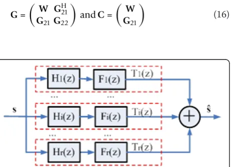
Otherwise, it can be observed that |Hi (ejω)| and |Fi (ejω)| only differ in a scaling factor and the sign of the power of the complex exponential argument. Hence, Ti (ejω) resembles |Hi (ejω)| in shape and its value can be given by |Ti (ejω)| = |Hi (ejω)|2/L. The pattern of the global FIR filter group is shown in Figure 1.
Besides, once alternative embedding procedure is adopted–the trajectory matrixS has Hankel structure but not Toeplitz structure (see [8,9] for example), the properties of Hi (ejω) and Fi(ejω) will interchange, i.e., the former corresponding to an anti-casual filter whereas the latter a casual filter.
3. Approximation of spectral decomposition
From Equations (10) (13), and (14), we learn that the entries of eigenvectoruicorrespond to the coefficients of the SSA FIR filter we proposed. Traditionally, eigen-vectors can be obtained via spectral decomposition algo-rithm, SVD on S or ED on G. Nevertheless, they are prohibitive for largeL. Here, we introduced two differ-ent approximate spectral decomposition methods for large dense matrices: Nyström method [11-15] and Col-umn-Sampling approximation [14-17]. Both of them are based on random sampling techniques which only oper-ate on a subset of the matrix and provide a powerful alternative for approximate spectral decomposition issue. As described in the previous section, the proposed algorithm focused working on theL×LSPSD matrixG = SSH, whose spectral decomposition is G =UΛUH. Suppose we randomly (so uniformly) samplel «L col-umns ofGwithout replacement. LetC denote theL×l
matrix formed by these sampled columns and Wthe l
×l matrix consisting of the intersection of these l col-umns with corresponding l rows of G. Based on this sampling, the columns and rows of G are rearranged. Thus, without loss of generality,Gand Ccan be written as follows:
G=
W GH21 G21 G22
andC=
W G21
(16)
Note thatW is also SPSD since Gis SPSD. Through performing ED or SVD on much smaller scale matrices
W andC, it can generate approximations of eigenpairs
U andΛ, denoted as U˜ and ˜ respectively, which we now describe.
The Nyström method is originally introduced to obtain numerical solutions to integral equations [25]. Then, the same idea is in turn applied to extend the solution of a reduced matrix eigen-decomposition pro-blem to approximate the eigenvectors of an SPSD matrix. The Nyström method provides an approxima-tion ofGby usingWand Cas follows
G≈ ˜G=CW−1CH =
W GH21
G21G21W−1GH21
(17)
where-1denotes the inverse of a matrix. Now define spectral decomposition W=UwwUHw, accordingly the approximations of eigenpairs are
˜
U:=
l
LCUw
−1
w (18a)
˜
:= L
lw (18b)
Unlike the Nyström method, the Column-Sampling method approximates the eigenpairs of Gby using the SVD ofCdirectly. It is initially motivated by exploring a simple and intuitive algorithm to compute a description of a low-rank approximation to a very large matrix, which is qualitatively faster than SVD [17]. Suppose the SVD ofCis C=UccVHc , then the approximated eigen-pairs ofGare obtained by
˜
U:=Uc (19a)
˜
:=
L
lc (19b)
Accordingly, it generates the approximation of Gby instituting (19a) and (19b) into G≈ ˜G=U˜˜U˜H:
G≈ ˜G=U˜˜U˜H
=Uc
L
lcU
H c = L l
CVc−c1
cCVc−c1
H = L lC
Vc−c1c−cHVHc
CH=
L
lC
Vc−cHVHc
CH
=C ⎛ ⎝l
L
CHC
1 2 ⎞ ⎠ −1 CH (20)
Here, we adopts Uc=CVc−c1 and CHC=Vc2cVHc . Compared with (17), it is obvious that the two methods Figure 1FIR eigenfilter description: Hi(z) are analysis filters and
have resembling forms with each other, the latter
replacesWin (14) with
l L
CHC
1 2.
The above sampling-based approximations adopt the most basic uniform sampling approach to pick outl col-umns from the original matrixG. Alternatively, some researchers derived several non-uniformly sampling approaches, i.e., selecting theith column with a weight that is proportional to either the corresponding diagonal element Giior the squared of the column-norm [13,17]. However, in the recent articles which have the guiding significance for the applications of sampling-based approximations on various problems, Kumor et al. [14,15] pointed that, for large dense matrices, the uni-form sampling without replacement approach, in addi-tion to being more efficient both in time and space, produces more effective approximations. Otherwise, Kumor et al. [15] summarized that the low-rank approx-imation issues can be classified into two groups–matrix projection and spectral reconstruction. Furthermore, the former approximations tend to be more accurate than the latter approximations when adopt sampling-based approximated methods. According to Equation (4), the RFI signal reconstruction belongs to the first kind. Based on the above analysis, using uniform sampling approach is a good choice.
In the basic SSA algorithm, the most time-consuming step is the spectral decomposition of theL×LmatrixG (or of theL×Ktrajectory matrixS). The computational cost of SVD onS is usually computed by the means of Golub and Reinsch algorithm [26], which requires O
(L2K+LK2+K3) multiplications. Using ED onG is even more prohibitive requiredO(L3) multiplications. Contra-rily, the Nyström method just needs to calculate the eigenpairs of the sampled submatrix ofGwhich requires
O(l3+l2L),r ≤ l, l3 required by ED on W andl2L for multiplication with C, and the Column-Sampling approximation needsO(L2l+Ll2+l3) multiplications for SVD onC. After measuring differences of floating-point numbers in arithmetic, we supply a comparison of con-crete CPU time when implementing different spectral decomposition algorithms on P-band real datasets, shown in Section 4.
4. Numerical experiments
In this section, we first perform numerical simulations for a time series to illustrate the methods discussed above. We consider a linear frequency modulation (LFM) signal, namely chirp signal, which is often used as SAR transmitting pulse [27]: secho= exp(-jπKt2), -T/2
≤t≤ T/2, where the pulse width T= 32μs, bandwidth
B= |K·T| is 9.6 MHz, the center frequency at zero and sampling frequencies is 39.6 NHz. All these parameters
are typical for a SAR transmitting pulse, except the sam-pling frequency. According to Nyquist principal 12 MHz is enough for the given bandwidth, but we adopt a high sampling frequency in order to obtain a comparatively
‘long’ time series which has 1,844 sample points. Three real sinusoidal signals as RFIs, whose center frequencies are 1.8, 3.2, and 3.5 MHz, respectively, have been added. To set two RFIs with similar frequencies, we can exam-ine the RFI suppression capability of SSA-FIR filter banks when RFIs with close frequencies present, and the signal-to-noise ratio is 40 dB.
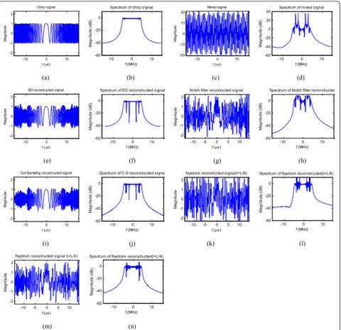
We adopt the above LFM signal as a calibrated signal, whose time domain waveform and corresponding power spectrum are shown in Figure 2a, b. After contaminated by RFIs (three sinusoidal signals), the time domain waveform and power spectrum of the mixed signal are shown in Figure 2c, d. One can see that the power of RFIs is about 40 dB higher than that of the calibrated signal. The method described in [5], we call it ‘ED method’ for convenience, and the Notch filtering method in [3] are chosen as contrast RFI suppression algorithms. We chooseL= 460 and because single
sinu-soidal signal sin(x)= 1 2
expjx−exp−jx
corre-sponds to rank 2, the rank isr = 6.
The reconstructed signals using accurate ED method are shown in Figure 2e, f, corresponding to time and fre-quency domains, respectively, and in Figure 2g, h, the performances of the Notch filtering method are repre-sented. Then, we first setl= floor(L/8) = 57, in this con-dition, the reconstructed signals using the Column-Sampling approximation and the Nyström method are shown in Figure 2i-l. One can see the Column-Sampling approximation works better and more approximately up to the ED reconstructed performance. Contrarily, the performance of the Nyström method is kind of unsatis-factory. It still leaves about 10 dB RFIs energy and the time domain signal wave is ‘chaotic’. Next, we set l= floor(L/4) = 115 and the reconstructed signal using the Nyström method are shown in Figure 2m, n. This time it works better, more RFIs energy is removed but its perfor-mance still little poorer than the Column-Sampling approximation’s, even when the latter with half of the sampling columns. The reason we will give through further numerical analysis. However, the Nyström method withl= floor(L/8) = 57 sampling columns still removes more RFIs energy than the Notch filtering method does. We can see the Notch caused some fre-quency spectrum fracture and lost the most useful signal. In the following, we monitor two quantificable criter-ions of the two approximated methods compared with the exact spectral decomposition, just for the eigenvec-tors u˜i
l
(18a) and (19a). First, we compute the cosines of princi-pal angles, between the exact and the approximate eigenvectors: cosAngle=ui2+u˜i2−ui− ˜ui2
ui2•u˜i2
,
i= 1,..l, which should be close to 1 for good approxima-tion. Here, ||•||2 denotes 2-norm. When the number of
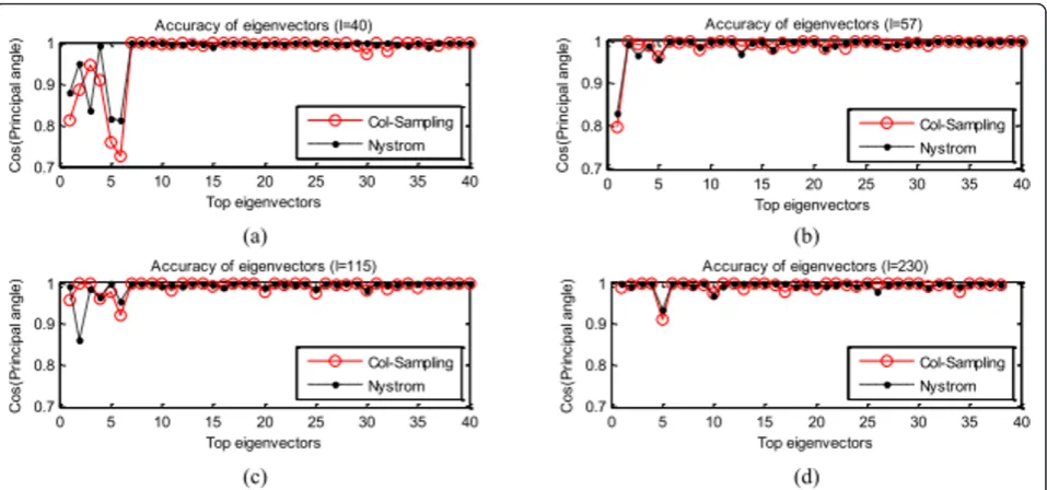
sampling columns varying, the error curves are shown in Figure 3 (in which we just give the top 40 results). We can see as the number of samples increasing, both of the Column-Sampling and the Nyström method
generate more accurate eigenvectors, and the accuracies of them are very close.
But, why their RFI suppression results are so different? In Table 1, we give the orthonormality error for differ-ent number of samples, which are measured by
Frobe-nius norm 10 log 10U˜U˜H−I
F
. We repeat the
excises for 50 times, and then compute the average deviation values. The mean deviation from Figure 2Time domain signal waveforms and corresponding normalized power specturms, in due order of Chirp signal, Chirp and sinusoidal mixed signal, and the reconstructed signals by the ED method, the Notch filtering method, the Column-Sampling
orthonormality decreases as the number of samples increases for both of the two methods. But, the ortho-normality error of the Nyström method is much larger than the Column-Sampling approximation. This is the reason for the poor Nyström method performance. When extrapolates eigenvectors of Gfrom eigenvectors ofW, the Nyström products lose orthonormality in this process.
The frequency responses of the associated filters with the first eight filter banks are shown in Figure 4. We adopt l = floor(L/4) = 115 columns for the Nyström method and half columns for the Column-Sampling approximation. Figure 4a-f shows that the first six filters have band-pass characteristics so that they mostly cap-ture the three sinusoidal harmonics of the mixed signals. Nevertheless, the other two filters shown in Figure 4g, h as contrast are much less important when reconstruct-ing signals. It illustrates that the two approximated methods are effective for constructing the SSA-FIR filter groups.
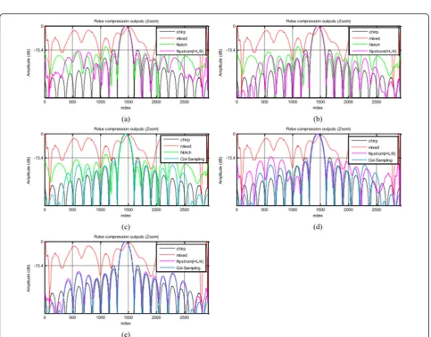
Then, we give the pulse compression results to illus-trate the targets resolution capability after using above multiple RFI suppression methods. All the reconstructed signals are filtered by a matched filter Hmatch = exp
(jπKt2), -T/2≤t≤ T/2 [27]. When the calibrated signal through the matched filter, it generates a waveform whose peak value of the main lobe is at least 13 dB higher than that of the highest pair of side lobes, and the magnitudes of other side lobe pairs are decreasing from center to both sides. Thus, the expected target can be distinguished. However, when there are RFIs, through matched filter we cannot differentiate the main lobe. We compared the compression results by pairs, the contrast waveforms are shown in Figure 5. One can see some sidelobes still higher than -13.4 dB line when using the Notch filtering method. Using the Nyström method with 115 samples we can obtain a satisfactory wave form, similar to the one when using the Column-Sam-pling approximation. But, when with only 57 samples, the Nyström method defeats the Notch filtering method by a narrow margin.
Next, we will detect the proposed algorithm in practi-cal scenario using real datasets which are collected by a P-band airborne SAR. These datasets include 16,384 pulses along the azimuth direction and each pulse has 10,240 sample points. It means each time the series has
M = 10240 entries. The main system parameters are reported in Table 2. The estimated Doppler center fre-quency is 6.1 Hz. Range-Doppler image focus algorithm [27] is adopted combined with motion compensation processing.
Our experiments are made on a PC equipped with Intel Core i3 CPU at 2.13 GHz with a duel core proces-sor, 4 GB of RAM memory. We adopt L= 2048 as the filter order, l = L/8 = 256 sampling columns for the Figure 3For different numbers of samples (l), cosines of principal angles between the exact and the approximated eigenvectors obtained by the Column-Sampling approximation and the Nyström method, respectively.
Table 1 Mean deviation from orthonormality for different number of samples
(dB) L= 40 L= 57 L= 115 L= 230
Figure 4Frequency response of the first eight zero-phase FIR filter banks constructed by the ED method, the Col-Sampling approximation and the Nyström method, respectively.
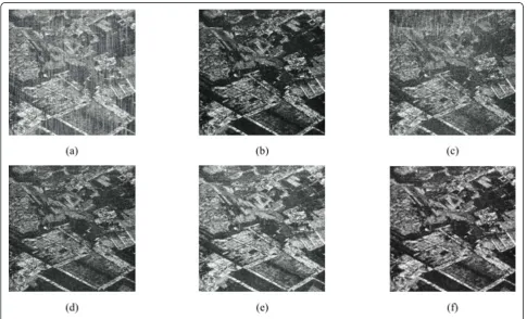
Column-Sampling approximation and the Nyström method, and an extra l =L/4 = 512 sampling number for the latter. The ED method and the Notch filtering method are still as contrast RFI suppression algorithms. For each pulse, the rank of the RFI subspace is given by Equations (5)-(7). Figure 6a interprets multiple narrow-band sources occurring at P-wavenarrow-band. The focused images after RFI suppression using the two contrast method–ED method and the Notch filtering method– are shown in Figure 6b, c respectively, and the other three images on the next line are obtained using the Column-Sampling approximation, the Nyström method with 256 samples, and with 512 samples, respectively. Figure 6b is considered as the optical reference image.
One can see that Figure 6c is blurred and the remaining interferences are visible. Surprisingly, from Figure 6e, we can see that the Nyström method with 256 samples makes much better performance than that of the Notch filtering. Although the simulation results in Figure 5a show it just slightly better than the latter. One possible reason is that the real scenario more RFIs exists, the Notch filtering method is so inflexible that makes more frequency gaps, and as shown in Figure 6d, f, the Col-umn-Sampling approximation and the Nyström method with 512 samples still have the similar suppression effects. Otherwise, we use the MATLAB commands‘tic’
and ‘toc’ to measure the required CPU running time when adopting different spectral decomposition meth-ods. The experimental results show that, for a single pulse, adopting ED method needs to run for 26.5694 s, the Column-Sampling approximation with l= 256 sam-ples needs 1.7012 s, the Nyström method with l= 512 samples needs 1.9712 s, and the Nyström method withl
= 256 samples only needs 0.3771 s.
5. Conclusions
In this article, we give analysis of that the RFI suppres-sion problem in SAR can be considered as one-dimen-sional stationary time series denoising problem.
Table 2 Main system parameters
Polarization HH
Bandwidth 85 MHz
Wavelength 0.75 m
Aircraft velocity 176.97 m/s Azimuth resolution 2 m
Range resolution 2 m
Pulse repetition frequency 1499.88 Hz
Near range 11861.57 m
Furthermore, by applying a linear invariant system the-ory, the RFI suppression task can be achieved expedi-ently by a zero-phase FIR filter whose coefficients are related to the eigenvectors of the input signal covariance matrix. Owing to the outputs being in phase with the inputs, phase preserving can be available through the proposed algorithm. What is more, in view of the large amount of SAR original data and high complexity of computing eigenvalues and eigenvectors, we first intro-duce two random sampling methods to speed up the SSA-FIR filter banks construction process. The results of simulations and practical experiments illuminate that the proposed filtering algorithm can be provided with both efficiency and validity.
Competing interests
The authors declare that they have no competing interests.
Received: 16 November 2011 Accepted: 9 May 2012 Published: 9 May 2012
References
1. M Soumekh, D Nobles, MC Wicks, JG Gerard, Signal processing of wide bandwidth and wide beam width P-3 SAR data.IEEE Trans Aerosp Electron Syst.4(37), 1122–1141 (2001)
2. T Miller, L Potter, J McCorkle, RFI suppression for ultra wideband radar.IEEE Trans Aerosp Electron Syst.33(4), 1142–1156 (1997)
3. H Kimura, T Nakamura, KP Papathanassiou, Suppression of ground radar interference in JERS-1 SAR data.IEICE Trans Commun.E87-B, 3759–3765 (2004)
4. X Luo, LMH Ulander, J Askne, G Smith, P-O Frolind, RFI suppression in ultra-wideband SAR systems using LMS filters infrequency domain.IET Electron Lett.37(4), 241–243 (2001). doi:10.1049/el:20010153
5. L Nguyen, T Ton, D Wong, M Soumekh, Adaptive coherent suppression of multiple wide-bandwidth RFI sources in SAR.Proc SPIE.5427, 1–16 (2004) 6. W Wang, LR Wyatt, Radio frequency interference cancellation for sea-state
remote sensing by high-frequency radar.IET Radar Sonar Navigat.5(4), 405–415 (2011). doi:10.1049/iet-rsn.2010.0041
7. N Golyandina, V Nekrutkin, A Zhigljavsky,Analysis of Time Series Structure: SSA and Related Techniques, Chapman & Hall, London, (2001)
8. TJ Harris, H Yuan, Filtering and frequency interpretations of singular spectrum analysis.Physica D.239, 1958–1967 (2010). doi:10.1016/j. physd.2010.07.005
9. PC Hansen, SH Jensen, FIR filter representations of reduced-rank noise reduction.IEEE Trans Signal Process.46(6), 1737–1741 (1998). doi:10.1109/ 78.678511
10. I Dologlou, G Carayannis, Physical interpretation of signal reconstruction from reduced rank matrices.IEEE Trans Signal Process.39(7), 1681–1682 (1991). doi:10.1109/78.134407
11. CKI Williams, M Seeger, Using the Nyström method to speed up kernel machines.NIPS.13, 682–688 (2001)
12. K Zhang, I Tsang, J Kwok, Improved Nyström low-rank approximation and error analysis. InProc ICML’08, New York, USA273–297 (2008)
13. P Drineas, MW Mahoney, On the Nyström method for approximating a Gram matrix for improved kernel-based learning.JMLR.6, 2153–2175 (2005) 14. S Kumor, M Mohri, A Talwalkar, Sampling techniques for the Nyström
method. InConference on Artificial Intelligence and Statistics JMLR: W&CP, Clearwater Beach, Florida, USA.5, 304–311 (2009)
15. S Kumor, M Mohri, A Talwalkar, On sampling-based approximate spectral decomposition. InProc 26th Annual International Conference on Machine Learning, Montreal, Canada553–560 (2009)
16. A Deshpande, L Rademacher, S Vempala, G Wang, Matrix approximation and projective clustering via volume sampling.Theor Comput.6, 225–247 (2006)
17. P Drineas, R Kannan, MW Mahoney, Fast Monte Carlo algorithms for matrices II: computing a low-rank approximation to a matrix.SIAM J Comput.36(1), 158–183 (2006). doi:10.1137/S0097539704442696
18. M Wax, T Kailath, Detection of signals by information theoretic criteria.IEEE Trans Acoust Speech, Signal Process.33(2), 387–392 (1985). doi:10.1109/ TASSP.1985.1164557
19. R Badeau, B David, G Richard, Selecting the modeling order for the ESPRIT high resolution method: an alternative approach. InIEEE International Conference on Acoustics, Speech, Signal Processing, Montreal, Quebec, Canada.
2, 1025–1028 (2004)
20. J-M Papy, Lathauwer DeL, SV Huffel, A shift invariance-based order-selection technique for exponential data modeling.IEEE Signal Process Lett.14(7), 473–476 (2007)
21. S Kritchman, B Nadler, Determining the number of components in a factor model from limited noisy data.Chemomet Intell Lab Syst.94(1), 19–32 (2008). doi:10.1016/j.chemolab.2008.06.002
22. K Johansson, Shape fluctuation and random matrices.Commun Math Phys.
209(2), 437–476 (2000). doi:10.1007/s002200050027
23. IM Johnstone, On the distribution of the largest principal components analysis. Ann Statist.29(2), 295–327 (2001). doi:10.1214/aos/1009210544 24. J Baik, G Ben Arous, S Péché, Phase transition of the largest eigenvalue for
non-null complex sample covariance matrices.Ann Probab.33(5), 1643–1697 (2005). doi:10.1214/009117905000000233
25. LM Delves, JL Mohamed,Computational Methods for Integral Equations, (Cambridge University Press, Cambridge, 1985)
26. G Golub, C Reinsch, Singular value decomposition and least squares solutions.Numer Math.14, 403–420 (1970). doi:10.1007/BF02163027 27. IG Cumming, FH Wong,Digital Processing of Synthetic Aperture Radar Data:
Algorithm and Implementation(Artech House, Inc., Boston, 2005)
doi:10.1186/1687-6180-2012-103
Cite this article as:Wanget al.:RFI suppression in SAR based on
filtering interpretation of SSA and fast implementation.EURASIP Journal
on Advances in Signal Processing20122012:103.
Submit your manuscript to a
journal and benefi t from:
7Convenient online submission
7Rigorous peer review
7Immediate publication on acceptance
7Open access: articles freely available online
7High visibility within the fi eld
7Retaining the copyright to your article