Combination of EEG Complexity and Spectral Analysis for Epilepsy Diagnosis and Seizure Detection

(1)

Volume 2010, Article ID 853434,15pages doi:10.1155/2010/853434

Research Article

Combination of EEG Complexity and Spectral Analysis for

Epilepsy Diagnosis and Seizure Detection

Sheng-Fu Liang,

1, 2

_{Hsu-Chuan Wang,}

1

_{and Wan-Lin Chang}

1

1_{Department of Computer Science and Information Engineering, National Cheng Kung University, Tainan 701, Taiwan} 2_{Institute of Medical Informatics, National Cheng Kung University, Tainan 701, Taiwan}

Correspondence should be addressed to Sheng-Fu Liang,[email protected]

Received 19 August 2009; Revised 20 January 2010; Accepted 6 April 2010

Academic Editor: Christophoros Nikou

Copyright © 2010 Sheng-Fu Liang et al. This is an open access article distributed under the Creative Commons Attribution License, which permits unrestricted use, distribution, and reproduction in any medium, provided the original work is properly cited.

Approximately 1% of the world’s population has epilepsy, and 25% of epilepsy patients cannot be treated suﬃciently by any available therapy. If an automatic seizure-detection system was available, it could reduce the time required by a neurologist to perform an oﬀ-line diagnosis by reviewing electroencephalogram (EEG) data. It could produce an on-line warning signal to alert healthcare professionals or to drive a treatment device such as an electrical stimulator to enhance the patient’s safety and quality of life. This paper describes a systematic evaluation of current approaches to seizure detection in the literature. This evaluation was then used to suggest a reliable, practical epilepsy detection method. The combination of complexity analysis and spectrum analysis on an EEG can perform robust evaluations on the collected data. Principle component analysis (PCA) and genetic algorithms (GAs) were applied to various linear and nonlinear methods. The best linear models resulted from using all of the features without other processing. For the nonlinear models, applying PCA for feature reduction provided better results than applying GAs. The feasibility of executing the proposed methods on a personal computer for on-line processing was also demonstrated.

1. Introduction

Epilepsy is one of the most common neurological disorders. Approximately 1% of the world’s population has epilepsy, and up to 5% of people may have at least one seizure during their lifetime [1]. Epilepsy is characterized by a sudden and recurrent malfunction of the brain, a “seizure” [2]. An electroencephalogram (EEG) is a record of the electrical potentials generated by the cerebral cortex’s nerve cells, and it has been an especially valuable clinical tool for the evaluation and treatment of epilepsy [3].

A continuous recording of the EEG lasting as long as one week is required to detect epilepsy. Examining the entire length of such EEG recordings by a well-trained neurologist is both tedious and time consuming. The time required by the neurologist to review extensive EEG data could be greatly reduced via assistance from a reliable automated seizure detection system. In addition, if an online seizure detection method was available, the system could signal healthcare professionals to provide immediate care when a seizure occurs, or it could drive a treatment device (e.g., an

electrical stimulator or a drug delivery device) to suppress the seizure and to enhance the patient’s quality of life [4,5].

(2)

(a)

(b)

(c)

(d)

500

mV

1 s (e)

Figure1: Exemplary EEG time series from five diﬀerent sets [22]. (a) normal eyes-open EEG (Set A), (b) Normal eyes-closed EEG (Set B), interictal EEG at (c) opposite (Set C) and (d) epileptogenic zones (Set D), and (e) ictal EEG (Set E) at epileptogenic zones.

seizure events by analyzing the spectra and/or the complexity of the EEG recordings.

The performance of an EEG-based seizure detection model may be aﬀected by at least four factors: (1) the EEG features, (2) the feature extraction/reduction methods, (3) the classifiers, and (4) the number of data classes to be classified. The objective of this study was to systematically evaluate the performance of current approaches described in the literature and to suggest a reliable, practical epilepsy detection method based on the findings of the evaluation. Because the dataset from Department of Epileptology, University of Bonn, Germany [21, 22], has been widely used for performance demonstration in many studies, the evaluation presented here focused on analyzing methods with this dataset for fair comparisons [8,12,14,18,23–34].

For EEG features, Srinivasan et al. successfully combined an approximate entropy (ApEn) analysis with neural net-works to discriminate between normal and ictal EEG signals, and the overall accuracy was as high as 100% [12]. The study presented here examined the capability of ApEn analysis to analyze multiclass EEGs, and the analysis’ performance was enhanced by combining ApEn analysis with the power of EEG subbands or autoregressive models [30]. Genetic algorithms [27] and principle component analysis [18] were compared to examine their ability to select features that are useful while using various linear and nonlinear methods for classification.

For the number of data classes to be classified, there are five datasetes in [21, 22], including normal eyes-open EEGs (Set A), normal eyes-closed EEGs (Set B), interictal EEGs at the opposite (Set C) and epileptogenic zones (Set

D), and ictal EEGs (Set E) at epileptogenic zones. For two-class two-classification, studies described in [8, 12, 14, 23–25] classified Set A and Set E, and their accuracies ranged from 92% to 100%. Studies described in [26,27] classified Set E and Sets A, B, C, and D, and their accuracies ranged from 96% to 97%. For three-class classification, studies described in [18,28–30] classified Set A, Set D (Set C in [30]), and Set E, and the accuracies ranged from 85% to 96%. Finally, the studies described in [31–34] classified the five datasetes, and the accuracies ranged from 89% to 99%. In our experiments, the seizure detection approaches were also used to classify two additional datasets: Set D and Set E; and Sets A and D and Set E.

The motivation of this study is to present a comprehen-sive study on state-of-the-art methods for seizure detection and propose a reliable and practical epilepsy detection method that can balance computational complexity and detection accuracy. The combination of complexity analysis and spectrum analysis on an EEG that can perform robust evaluations on the collected data is proposed. Applying principle component analysis (PCA) for feature reduction and utilizing radial-basis-function support vector machine as the classifier are developed for multiclass EEG discrimina-tion. For online seizure detection, the temporal and spectral features are integrated with the linear classifiers and can be easily implemented on current processing platforms and perform with high accuracy and with low computational cost. In addition, it is feasible for the system to responsively drive a treatment device, such as an electrical stimulator or a drug delivery device, to suppress the seizures.

2. Dataset

This study utilized the dataset from Department of Epilep-tology at the University of Bonn, Germany [22,23], because many seizure detection methods have been proposed and evaluated with this dataset. It contains normal EEGs of healthy subjects, interictal EEGs of epileptic subjects, and ictal EEGs of epileptic subjects. Each set contains 100 single-channel EEG segments with a duration of 23.6 s and a sampling frequency of 173.61 Hz. Each segment consists of 4,096 samples. Segments from Sets A and B contain normal EEGs taken using surface electrodes on five healthy people with their eyes open and closed, respectively. Sets C and D contain interictal EEGs taken from five epileptic patients using intracranial electrodes placed at the opposite and epileptogenic zones, respectively. Set E contains ictal EEGs taken from five epileptic patients using intracranial elec-trodes placed at the epileptogenic zone. The type of epilepsy was diagnosed as temporal lobe epilepsy. The exemplary EEG segments from each set are shown inFigure 1.

3. Methods

(3)

0 20 40 60 80 100 120 140 160

N

u

mber

of

w

indo

w

s

0 0.2 0.4 0.6 0.8 1 1.2 1.4 1.6 1.8 2 Approximate entropy value

Normal Interictal Ictal

(a)

0 50 100 150 200 250

N

u

mber

of

w

indo

w

s

0 0.2 0.4 0.6 0.8 1 1.2 1.4 1.6 1.8 2 Sample entropy value

Normal Interictal Ictal

(b)

Figure2: Applying entropy analysis to the normal, interictal, and ictal EEG datasets. (a) Results by approximate entropy. (b) Results by sample entropy.

three elements. The results of the evaluation were used to suggest methods for achieving a practical epilepsy detection method.

For EEG features, the approximate entropy (ApEn) analysis was evaluated for its ability to analyze multiclass EEGs, and the performance of ApEn analysis was enhanced by incorporating the power of EEG subbands or autore-gressive models [30]. Genetic algorithms [27] and principle component analysis [18] were compared for their ability to select features while using various linear and nonlinear methods for classification.

3.1. Spectral and Entropy Analysis

3.1.1. Approximate Entropy (ApEn). Approximate entropy

(ApEn) is a measure that quantifies the regularity or the predictability of a time series [35]. ApEn accounts for the temporal order of points in a time sequence and is therefore a preferred measure of randomness or regularity. It has also been used recently for the detection of epilepsy [8, 12]. Smaller values of ApEn imply a greater likelihood that similar patterns of measurements will be followed by additional similar measurements [35].

In addition to diagnosis such as discriminating between the EEGs of healthy people and the epileptic-seizure EEGs of patients [12], the ability to discriminate between the ictal and nonictal EEGs of epileptic patients is also important for some practical applications, such as seizure warning systems or closed-loop seizure control systems [5].Figure 2(a)shows the distribution, the means, and the standard deviations of ApEn values corresponding to three datasetes: the normal scalp EEGs of healthy subjects (Set A), the interictal EEGs of epileptic subjects (Set D), and the ictal EEGs of epileptic

subjects (Set E). The data length of each nonoverlapping window for ApEn calculation was 512 points, and the other ApEn parameters were r = 0 and m = 1 [12]. Based on these data, ApEn was a good index for discriminating between normal (Set A) and ictal EEGs (Set E). However, the ApEn values of the interictal EEGs overlapped with those of the normal and the ictal EEGs. Figure 2(b) shows the results from the sample entropy analysis method [36] that was proposed to eliminate bias caused by self-matching. The values from sample entropy analysis corresponding to the interictal EEGs overlap with those of the normal EEGs, and ApEn analysis performs better than the sample entropy method for discriminating between normal and ictal EEGs. Thus, to improve the performance of epileptic seizure detection, it is required to combine additional, complementary features to ApEn analysis. Spectral features and the autoregressive model are compared for this purpose.

3.1.2. Spectral Analysis. The EEG power spectra calculated

using a fast Fourier transform (FFT) were normalized to a logarithmic scale. The 0–60 Hz frequency range was continuously segmented into 15 subbands, and the averaged EEG log-power spectrum from each sub-band (with a 4 Hz bandwidth) was extracted to generate the spectral features used by the classifying method. The feature for each sub-bandi(for 0≤i≤14) was calculated by

PSi=Mean

PSf, 4·i < f ≤4·(i+ 1), (1)

where PS(f) is the log power of frequencyf.Combined with a time domain feature (i.e., the approximate entropy), a total of 16 features were used.

(4)

the approximate entropy analysis and spectral analysis was applied to each subwindow. The feature values of the EEG segment were the median values of the ApEn and the band powers for each of divided subwindows. Assuming that the number of data points of an EEG segment to be classified is

N, the resultant ApEn is

ApEn=MEDApEnk

, k=1, 2,. . . N/128, (2)

and the power of theith band is

PSi=MED

PSi,k

, (3)

where PSi,k represents the power of theith band at thekth sub-window [37].

3.1.3. Autoregressive Model. The autoregressive (AR) model

is a parametric model used to describe stationary time series, and it is also a popular tool for EEG analysis [38]. AR models represent the current signal as the weighted sum of its previous values and the white noise. The determination of the weights is based on the least mean square (LMS) criteria. For the analysis presented here, Akaike’s information criterion [39] was used to determine the appropriate order of the AR model, which was 20. The weights of the AR model and the ApEn analysis (a total of 21 features) were combined as the set of features for use by the classifiers and were compared with the spectral features.

3.2. Feature Reduction. Principle component analysis and

genetic algorithms have been utilized to perform feature reduction in seizure detection methods [18, 27]. Here, these two methods have been used in conjunction with the combination of ApEn analysis and spectral power analysis for feature reduction, and the results are compared to those obtained when examining the original 16 features without any processing.

3.2.1. Principle Component Analysis. Principal component

analysis transforms a set of correlated variables into a new set of uncorrelated variables that can use fewer dimensions to express the relevant information contained in the obser-vation data. It has also been widely used in EEG analysis for dimension reduction or for feature extraction [18,37]. For this analysis, PCA was applied to the 16 features (ApEn and the powers of the 15 subbands), and the resultant principle components (PCs) were fed to the classifiers for evaluation. The number of PCs was determined based on the best performance of each classifier [18].

3.2.2. Genetic Algorithm. A Genetic Algorithm (GA) is an

adaptive heuristic search algorithm. It starts with an initial population of fixed-length individuals (chromosomes). The evolution process is governed by selection, crossover, and mutation [40] of the parents to generate the children’s generation. A fitness function is defined to evaluate how well a solution (i.e., the individuals) solves the problem. Here, the settings and the procedure for the GA followed the approach proposed in [27] for seizure detection. At initialization, the

population size was set at 20. Each individual consisted of 16 genes that represented each of the 16 features (i.e., the ApEn and the powers of the 15 subbands). The genes were allowed to have a value of 0 or 1. The value of 1 implied that the corresponding feature was selected, and a value of 0 implied that the corresponding feature was excluded. The fitness value of an individual was defined as the inverse value of the classification error. Two of the individuals (the elites) in the current generation were quarantined to survive to the next generation without any modifications. In each generation, 80% of the individuals in the population, excluding the elites, were created through a crossover operation. The remaining 20% were generated through mutation. The algorithm was allowed to run for a maximum of 100 generations. The stop criteria for the algorithm were set such that the algorithm would halt if there were no improvements in the fitness values from 20 consecutive generations [27].

3.3. Classification. To evaluate and compare the performance

of analysis methods, four linear and nonlinear methods were utilized to classify the extracted features as a seizure or a Nonseizure event. The four evaluated methods were linear least squares [41], linear discriminate analysis [42], a backpropagation (BP) neural network [43], and the support vector machine with either the linear (LISVM) or the radial-basis function kernels (RBFSVM) [44].

The linear least squares (LLS) method finds a best fitting linear model that minimizes the mean square error between the system output and the desired output. Mathematically, it can be stated as finding an approximate solution to an overdetermined system of linear equations. Because the model output is only the weighted sum of the input features, it is suitable for implementation using processors without high computing power or for use in online processing. Linear discriminant analysis (LDA) uses a hyperplane to find the linear combination of features that best separates two or more classes of objects or events. Usually, the within-class, between-within-class, and mixture scatter matrices are used to formulate the criteria for searching the hyperplane so that the distance between the classes’ means is minimized and the interclass variance is maximized [45,46].

Backpropagation (BP) neural networks are widely used nonlinear models for pattern recognition and classification problems. BP is a multilayer perceptron that is composed of several layers of neurons. The error between the desired output and the network output is backpropagated from the output layer to the hidden and input layers to update the weights for network training based on the gradient-descent method. Here, a 3-layer feedforward neural network was utilized, and the number of neurons in the hidden layer was 20. The log-sigmoid function was used as the activation function of the hidden and output layers. The learning constant was 0.1 for network training and iteration number is 2000 for network training.

(5)

Table1: Groupwise average accuracies of various feature extraction methods combined with various classifiers applied to classify sets A, D, and E (standard deviations are noted in parentheses).

Classifier Feature selection A D E Accuracy

LLS

All features 100.00 (0.0) 95.00 (3.9) 95.50 (1.6) 96.83 (1.2)

GA 99.25 (1.2) 94.50 (3.3) 94.75 (3.6) 96.17 (1.9)

ApEn + AR model 98.50 (2.4) 95.50 (2.6) 95.50 (3.1) 96.50 (1.3)

LDA

All features 100.00 (0.0) 94.50 (3.9) 95.75 (1.7) 96.75 (1.1)

GA 99.50 (1.1) 95.00 (4.4) 94.50 (2.3) 96.33 (1.9) ApEn + AR model 97.50 (2.6) 96.00 (2.9) 95.75 (3.1) 96.41 (1.6)

BP

All features 98.75 (3.1) 96.50 (2.9) 97.00 (2.0) 97.42 (1.4) PCA 100.0 (0.0) 97.75 (1.8) 97.00 (2.6) 98.25 (1.5)

GA 98.50 (1.7) 91.50 (5.2) 97.50 (2.4) 95.83 (2.0)

ApEn + AR model 99.25 (1.2) 93.00 (5.5) 89.50 (6.0) 93.92 (3.0)

LISVM

All features 99.50 (1.1) 97.00 (2.6) 98.25 (1.2) 98.25 (1.1)

PCA 99.75 (0.8) 98.00 (2.0) 97.25 (1.4) 98.33 (0.6)

GA 98.75 (2.1) 93.50 (5.0) 98.00 (1.1) 96.75 (1.7)

ApEn + AR model 99.75 (0.8) 94.25 (3.1) 94.50 (5.0) 96.17 (2.2)

RBFSVM

All features 99.75 (0.8) 97.75 (1.8) 97.75 (1.4) 98.42 (0.8)

PCA 99.75 (0.8) 98.25 (1.8) 98.00 (1.6) 98.67 (0.7)

GA 99.50 (1.6) 95.00 (3.7) 96.50 (2.7) 97.00 (1.7) ApEn + AR model 99.75 (0.8) 92.25 (3.2) 91.75 (3.9) 94.58 (1.8)

Table2: Groupwise average accuracies of various feature extraction methods combined with various classifiers applied to classify sets A, B, C, D, and E (standard deviations are noted in parentheses).

Classifier Feature

Selection A B C D E Accuracy

LLS All features 94.75 (3.6) 88.75 (5.0) 51.00 (8.6) 60.00 (8.0) 92.25 (3.6) 77.95 (1.7)

LDA All features 96.00 (2.9) 88.25 (5.3) 51.00 (8.6) 62.00 (8.1) 94.25 (4.1) 78.30 (1.7)

BP All features 95.75 (3.1) 91.50 (3.8) 59.25 (8.8) 63.75 (9.3) 94.00 (2.7) 80.85 (1.5) PCA 94.75 (4.9) 92.50 (3.3) 63.25 (7.0) 70.50 (9.5) 93.00 (2.8) 82.80 (2.5)

LISVM All features 94.75 (6.5) 92.00 (4.4) 59.50 (5.8) 64.50 (6.5) 95.25 (1.4) 81.20 (1.4) PCA 94.50 (4.4) 91.75 (4.7) 62.50 (7.7) 63.00 (9.1) 94.50 (3.5) 81.25 (2.2)

RBFSVM All features 97.00 (4.4) 93.00 (3.5) 71.75 (6.5) 70.00 (8.7) 96.00 (3.4) 85.55 (2.0) PCA 94.25 (7.3) 92.50 (3.7) 75.75 (7.4) 72.00 (6.7) 95.00 (3.3) 85.90 (2.4)

Table3: Total number of windows corresponding to various window lengths used for training and testing the classifiers for seizure detection.

Sets Window size Number of windows for training Number of windows for testing

Nonseizure Seizure Nonseizure Seizure

D-E

173 1380 1380 920 920

256 960 960 640 640

512 480 480 320 320

AD-E

173 2760 1380 1840 920

256 1920 960 1280 640

512 960 480 640 320

ABCD-E

173 5520 1380 3680 920

256 3840 960 2560 640

(6)

Table4: Sensitivity, specificity, and accuracy of combining various feature extraction methods with various classifiers to distinguishing between Set E (ictal) and Set D (interictal).

Window size Classifier Feature selection Sensitivity Specificity Accuracy

173

LLS

All features 95.98 (1.4) 95.14 (1.0) 95.56 (0.8)

GA 95.90 (1.3) 94.66 (1.6) 95.28 (0.9) ApEn + AR model 95.88 (0.8) 94.85 (1.6) 95.36 (0.8)

LDA

All features 95.98 (1.4) 95.14 (1.0) 95.56 (0.8)

GA 95.79 (0.9) 94.82 (1.3) 95.30 ( 0.7) ApEn + AR model 95.88 (0.8) 94.85 (1.6) 95.36 (0.8)

BP

All features 95.90 (0.9) 95.41 (1.2) 95.66 (0.7)

PCA 95.89 (1.0) 94.65 (1.2) 95.27 (0.6) GA 95.67 (1.3) 94.49 (1.9) 95.08 (1.1) ApEn + AR model 93.47 (2.0) 94.95 (1.4) 94.21 (1.2)

LISVM

All features 95.68 (1.0) 95.62 (1.2) 95.65 (0.8)

RBFSVM

All features 96.04 (1.1) 95.29 (1.2) 95.67 (0.7)

256

LLS

All features 95.48 (1.8) 96.20 (1.5) 95.84 (1.2)

GA 95.27 (1.7) 95.88 (1.3) 95.57 (1.2) ApEn + AR model 96.23 (0.6) 95.08 (2.2) 95.66 (1.2)

LDA

All features 95.48 (1.8) 96.20 (1.5) 95.84 (1.2)

GA 94.64 (1.8) 96.34 (1.2) 95.49 (1.2) ApEn + AR model 96.23 (0.6) 95.08 (2.2) 95.66 (1.2)

BP

All features 96.03 (1.2) 95.70 (1.3) 95.87 (0.9) PCA 95.72 (1.1) 96.03 (1.3) 95.88 (0.6)

GA 95.75 (1.4) 95.03 (1.5) 95.39 (0.9) ApEn + AR model 93.34 (2.5) 95.58 (1.6) 94.46 (1.3)

LISVM

All features 95.61 (1.3) 96.41 (1.4) 96.01 (0.9)

PCA 95.19 (1.2) 96.11 (1.6) 95.65 (1.0) GA 95.19 (1.2) 95.91 (1.4) 95.55 (0.7) AR model 94.67 (1.7) 95.06 (1.9) 94.87 (1.4)

RBFSVM

All features 96.34 (1.4) 96.53 (1.3) 96.44 (0.9)

512

LLS

All features 96.03 (2.0) 96.56 (1.8) 96.30 (1.4)

GA 95.91 (2.0) 96.47 (1.8) 96.19 (1.4) ApEn + AR model 96.44 (0.8) 95.38 (2.1) 95.91 (1.1)

LDA

All features 96.30 (2.0) 96.56 (1.8) 96.30 (1.4)

GA 96.03 (1.9) 96.03 (1.7) 96.03 (1.4) ApEn + AR model 96.44 (0.8) 95.38 (2.1) 95.91 (1.1)

BP

All features 96.63 (1.3) 95.88 (1.7) 96.25 (1.0)

LISVM

All features 96.91 (1.2) 96.59 (1.6) 96.75 (1.0) PCA 94.47 (3.6) 98.57 (0.8) 97.75 (0.6)

(7)

Table4: Continued.

Window size Classifier Feature selection Sensitivity Specificity Accuracy

RBFSVM

All features 97.22 (1.3) 96.63 (1.6) 96.92 (1.1)

PCA 97.00 (2.0) 99.18 (0.6) 98.74 (0.5)

GA 96.44 (1.5) 96.13 (1.4) 96.28 (0.9) ApEn + AR model 92.00 (4.1) 94.53 (2.6) 93.27 (2.3)

increase the method’s generalization capabilities. The SVM performs structural risk minimization and creates a classifier with a minimized Vapnik-Chervonenkis (VC) dimension. When the VC dimension is low, the expected probability of error is low and ensures a good generalization. The SVM can also simultaneously minimize the empirical risk and the expected risk of pattern classification problems [47]. For the analysis presented here, two kinds of kernels, the linear kernel and the radial-basis function, were used. The RBF kernel nonlinearly maps samples into a higher dimensional space to handle cases where the relation between class labels and attributes is nonlinear. The parameter settings used were the following: a penalty parameter, C =2; a variance,σ = 0.5 for RBFSVM; and C=1 for LISVM.

4. Results

The experiments consisted of two parts: (1) Epilepsy Diag-nosis based on classification of three or five EEG datasetes, including normal EEGs, interictal EEGs, and ictal EEGs and (2) Seizure Detection based on classifying the windowed EEG trials as ictal or nonictal. The results demonstrated the feasibility of the seizure detection method for use in online seizure detection. This experiment contained three subexperiments. The first was to distinguish ictal EEGs (Set E) and nonictal EEGs (Sets A and D). The second was to distinguish ictal EEGs (Set E) and interictal EEGs (Set D). The third was to distinguish ictal EEGs (Set E) and nonictal EEGs (Sets A, B, C, and D) when all of the datasets provided in [22] are used.

4.1. Classification. Table 1 shows the average accuracies obtained by combining various feature extraction methods and classifiers to classify the three EEG datasetes, including the normal EEGs (Set A), the interictal EEGs (Set D), and the ictal EEGs (Set E). Most of the seizure-detection methods were evaluated with Sets A, D, and E without using Sets B and C [18, 28, 29]. Set B consists of normal EEGs taken from subjects with closed eyes that will induce specific alpha rhythms. Set C consists of interictal EEGs taken with intracranial electrodes at the opposite side of the epileptic zones, but a temporal-lobe seizure is regarded as a focal seizure.

In the experiments, 60% of the datasetes were randomly selected for training and the remaining data were used for testing the performance of the methods. The procedures were repeated 10 times to obtain the average performance results and their standard deviations (noted in parentheses).

By combining the temporal and spectral features of the EEG signals, the average accuracies of the linear models were remarkable and close to 97%. The use of PCA enhanced the best average classification accuracies of BP and

SVM.Figure 3shows the average variation in classification

accuracies versus the number of principle components with respect to various classifiers. Applying the PCA method did not improve the average accuracy of LLS or LDA and it required more computation for the linear classifiers, so PCA will not be combined with the linear classifiers in the following experiments. However, PCA did improve either the dimension reduction or the accuracy improvement of BP and SVM. The RBFSVM method had the highest average accuracy when combined with PCA. The GA did not improve the average accuracies for all classifiers. The results obtained by combining ApEn analysis with the AR model were worse than the results of combining ApEn analysis and EEG spectral features.

Table 2 shows the average accuracies of applying the

linear and nonlinear classifiers to classify all of the five EEG datasetes. The results show that nonlinear classifiers perform much better than the linear classifiers if the number of data classes increases. In our experiments, the best result among the ten tests for each classifier can be higher than 80% and the best result of RBFSVM can reach 90%.

4.2. Toward an Online Seizure Detection System. To evaluate

the feasibility of online operation of the seizure detection methods, all of the segments of the datasetes were divided into nonoverlapping windows with 173-, 256-, and 512-point window lengths. The trial numbers corresponding to various window lengths for training and for testing are shown inTable 3. Three combinations of the datasets were set to distinguish between ictal and nonictal EEGs, including (1) Set D versus Set E, (2) Sets A and D versus Set E, and (3) Sets A, B, C, and D versus Set E. Tables 4–6 show the results from combining various feature extraction methods with various classifiers and applying them to the three cases, respectively. Sensitivity (SE), specificity (SP), and accuracy (AC) are defined as

SE= TP

TP + FN, (4)

SP= TN

TN + FP, (5)

AC= TP + TN

(8)

Table5: Sensitivity, specificity, and accuracy of combining various feature extraction methods with various classifiers to distinguishing between Set E (ictal windows) and Sets (A, D) (normal and interictals).

Window size Classifier Feature Selection Sensitivity Specificity Accuracy

173

LLS

All features 93.61 (2.1) 97.79 (0.8) 96.40 (0.6)

GA 92.85 (2.5) 97.69 (0.8) 96.08 (0.7) ApEn + AR model 92.53 (1.8) 98.10 (0.7) 96.25 (0.7)

LDA

All features 95.60 (1.4) 97.32 (0.9) 96.74 (0.5)

GA 95.67 (1.7) 96.99 (1.2) 96.55 (0.7) ApEn + AR model 94.03 (1.7) 97.55 (0.8) 96.38 (0.7)

BP

All features 94.59 (2.5) 97.42 (1.2) 96.47 (0.8) PCA 94.26 (2.3) 97.91 (0.8) 96.70 (0.8)

GA 89.34 (3.9) 98.45 (0.5) 96.63 (0.5) ApEn + AR model 93.97 (2.4) 97.38 (1.1) 96.24 (0.7)

LISVM

All features 94.75 (1.8) 97.84 (0.9) 96.81 (0.5) PCA 93.91 (2.2) 97.64 (0.8) 96.40 (0.6)

GA 93.97 (2.6) 97.62 (1.0) 96.40 (0.9) ApEn + AR model 94.36 (2.1) 97.42 (1.0) 96.40 (0.7)

RBFSVM

All features 95.22 (1.9) 97.98 (0.9) 97.06 (0.6) PCA 98.85 (1.9) 97.90 (0.8) 96.88 (0.6)

GA 94.75 (2.2) 97.72 (1.1) 96.73 (0.8) ApEn + AR model l 94.07 (1.8) 97.23 (1.1) 96.18 (0.6)

256

LLS

All features 94.92 (1.5) 98.37 (0.8) 97.22 (0.5)

GA 94.33 (1.7) 98.15 (0.7) 96.88 (0.4) ApEn + AR model 93.39 (1.8) 98.08 (0.8) 96.49 (0.7)

LDA

All features 96.06 (1.2) 97.77 (1.0) 97.20 (0.5)

GA 95.92 (1.8) 97.24 (1.3) 96.80 (0.6) ApEn + AR model 96.36 (1.7) 97.51 (0.9) 96.46 (0.7)

BP

All features 95.89 (2.1) 97.79 (1.4) 97.16 (0.9) PCA 95.25 (1.5) 98.58 (0.7) 97.47 (0.5)

GA 95.75 (3.0) 97.35 (1.4) 96.82 (1.1) ApEn + AR model 94.16 (2.6) 97.80 (1.2) 96.58 (0.6)

LISVM

All features 96.19 (1.8) 98.23 (1.0) 97.55 (0.6)

RBFSVM

All features 96.88 (1.8) 98.41 (1.0) 97.90 (0.7)

512

LLS

All features 95.59 (1.3) 98.58 (0.7) 97.58 (0.3)

GA 95.50 (2.0) 98.39 (1.0) 97.43 (0.9) ApEn + AR model 93.94 (2.0) 98.13 (0.8) 96.73 (0.7)

LDA

All features 97.03 (1.0) 98.13 (0.9) 97.76 (0.4)

GA 96.81 (1.7) 97.78 (0.9) 97.46 (0.9) ApEn + AR model 94.59 (1.9) 97.77 (0.9) 96.71 (0.7)

BP

All features 97.44 (1.5) 97.81 (1.4) 97.69 (0.9) PCA 96.78 (1.6) 98.47 (0.9) 97.90 (0.5)

GA 95.91 (2.7) 98.05 (1.3) 97.33 (1.0) ApEn + AR model 95.00 (1.8) 97.88 (1.0) 96.92 (0.6)

LISVM

All features 97.28 (1.4) 98.66 (0.8) 98.20 (0.5)

(9)

Table5: Continued.

Window size Classifier Feature Selection Sensitivity Specificity Accuracy

RBFSVM

All features 97.53 (1.4) 98.73 (1.0) 98.33 (0.7)

PCA 97.44 (1.5) 98.77 (0.9) 98.32 (0.6)

GA 97.37 (1.9) 98.53 (0.9) 98.15 (0.8) ApEn + AR model 93.63 (2.4) 97.28 (1.3) 96.06 (1.0)

60 65 70 75 80 85 90 95 100

Classification

ac

cur

acy

(%)

0 2 4 6 8 10 12 14 16

Number of PCs LDA

LLS

(a)

60 65 70 75 80 85 90 95 100

Classification

ac

cur

acy

(%)

0 2 4 6 8 10 12 14 16

Number of PCs BP

LISVM RBFSVM

(b)

Figure3: Variations in classification accuracies versus number of principle components with respect to various classifiers for epilepsy diagnosis. (a) LDA and LLS. (b) BP, LISVM, and RBFSVM.

where TP is the true positive, the total number of correctly detected positive events; TN is the true negative, the total number of correctly detected negative events; FP is the false positive, the total number of erroneously positive detections (i.e., false alarms); and FN is the false negative, the total number of erroneously negative detections (i.e., missed detections).

Table 4shows that the performance of linear classifiers

was similar to the nonlinear models, and the average accuracy of seizure detection could reach roughly 96% for the 173-pt EEG windows (a data window of approximately 1 second). The detection accuracy increased to 98% for the 512-pt EEG windows (a data window of approximately 3 seconds). For the linear models, utilizing all of the features obtained the best accuracy, and features extracted by PCA provided for the best accuracy from the nonlinear models. The RBFSVM had the highest average accuracy when combined with PCA.

The average accuracies in Tables5and6are somewhat higher than those in Table 4 because the specificity was improved by including more datasets (i.e., Set A or Sets A, B, C) to Set D in the nonictal class. However, the sensitivity values were reduced due to uneven numbers of data points.

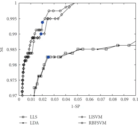
LDA had a more stable sensitivity than LLS and is close to the sensitivity of RBFSVM. For these experiments, the BP had two output nodes representing ictal and nonictal events, respectively. The class belonging to the output node that had the higher output value was regarded as the classified result for each input vector. For the linear models and the SVMs, the threshold was set as the “knee point” of the receiver operation characteristic (ROC) curve corresponding to the training data (Figure 4). To avoid bias, no testing data were used to determine the threshold.

(10)

Table6: Sensitivity, specificity, and accuracy of combining various feature extraction methods with various classifiers to distinguishing between Set E (ictal windows) and all nonictal windows (Sets A, B, C, and D).

Window size Classifier Selection feature Sensitivity Specificity Accuracy

173

LLS

All features 88.40 (2.9) 98.67 (0.3) 96.62 (0.4) GA 89.03 (2.6) 98.67 (0.3) 96.74 (0.4)

ApEn + AR model 86.13 (3.5) 99.17 (0.2) 96.56 (0.6)

LDA

All features 93.71 (1.8) 97.90 (0.5) 97.07 (0.3)

GA 93.84 (1.6) 97.82 (0.5) 97.03 (0.3) ApEn + AR model 89.87 (3.1) 98.53 (0.3) 96.80 (0.5)

BP

All features 89.46 (3.5) 98.57 (0.4) 96.74 (0.5) PCA 92.26 (2.2) 98.56 (0.3) 97.30 (0.4)

GA 89.34 (3.9) 98.45 (0.5) 96.63 (0.5) ApEn + AR model 91.83 (3.1) 98.67 (0.5) 97.30 (0.5)

LISVM

All features 92.75 (1.9) 98.43 (0.5) 97.29 (0.3)

RBFSVM

All features 93.09 (1.9) 98.61 (0.5) 97.50 (0.3)

256

LLS

All features 89.23 (3.3) 99.35 (0.3) 97.33 (0.6)

GA 89.33 (3.1) 99.30 (0.3) 97.31 (0.5) ApEn + AR model 86.72 (3.8) 99.24 (0.3) 96.74 (0.7)

LDA

All features 93.45 (2.2) 98.73 (0.4) 97.67 (0.3) GA 94.03 (2.2) 98.66 (0.5) 97.73 (0.4)

ApEn + AR model 90.14 (3.5) 98.67 (0.3) 96.96 (0.7)

BP

All features 92.27 (3.2) 98.68 (0.6) 97.40 (0.4) PCA 92.55 (2.3) 99.09 (0.5) 97.78 (0.4)

GA 89.84 (3.9) 98.83 (0.6) 97.03 (0.7) ApEn + AR model 92.39 (2.7) 98.91 (0.5) 97.61 (0.5)

LISVM

All features 93.30 (2.2) 98.97 (0.6) 97.84 (0.3) PCA 93.00 (2.4) 98.96 (0.5) 97.77 (0.3)

GA 92.97 (2.4) 98.84 (0.6) 97.67 (0.4) ApEn + AR model 92.47 (2.6) 98.77 (0.4) 97.51 (0.5)

RBFSVM

All features 94.69 (1.9) 99.10 (0.6) 98.21 (0.5)

512

LLS

All features 91.40 (2.7) 99.42 (0.2) 97.82 (0.5)

GA 90.91 (4.2) 99.32 (0.3) 97.64 (0.7) ApEn + AR model 87.31 (0.4) 99.32 (0.3) 96.92 (0.8)

LDA

All features 94.25 (2.1) 99.04 (0.4) 98.08 (0.3)

GA 94.66 (2.2) 98.88 (0.5) 98.04 (0.4) ApEn + AR model 90.59 (3.5) 98.79 (0.4) 97.15 (0.7)

BP

All features 92.16 (3.6) 98.72 (0.5) 97.41 (0.7) PCA 94.94 (2.0) 99.09 (0.5) 98.26 (0.4)

GA 93.63 (2.9) 98.95 (0.3) 97.88 (0.4) ApEn + AR model 93.75 (2.4) 98.88 (0.6) 97.85 (0.5)

LISVM

All features 95.28 (1.8) 99.13 (0.5) 98.36 (0.4) PCA 94.72 (2.1) 99.07 (0.5) 98.20 (0.3)

(11)

Table6: Continued.

Window size Classifier Selection feature Sensitivity Specificity Accuracy

RBFSVM

All features 95.78 (1.8) 99.19 (0.6) 98.51 (0.5)

PCA 95.78 (1.8) 99.19 (0.6) 98.51 (0.5)

GA 95.47 (1.4) 99.07 (0.5) 98.35 (0.4)

ApEn + AR model 92.43 (3.4) 98.58 (0.6) 97.35 (0.7)

Table7: Time consumption of the proposed method implemented on a personal computer (PC) to analyze EEG data corresponding to diﬀerent data length. The program was coded by C language. The processor is Intel core 2 6600 operated in 2.4 GHz and the RAM size is 2 G.

Window size Execution time (ms) FFT Entropy LLS/LDA Total

173 (1 s) 1000 cycles/one cycle 109/0.109 ms 422/0.422 ms 16/0.016 ms 547/0.547 ms

256 (1.48 s) 1000 cycles/one cycle 125/0.125 ms 453/0.453 ms 16/0.016 ms 594/0.594 ms

512 (2.95 s) 1000 cycles/one cycle 172/0.172 ms 844/0.844 ms 16/0.016 ms 1032/1.032 ms

Table8: A comparison of performances of the various methods for detection of epileptic seizures applied to the dataset from [21,22] (reproduced from [26,34]).

Classes Authors (year) Method Dataset Accuracy

2

Nigam et al. [23] (2004) Nonlinear preprocessing filter, diagnostic artificial neural

network (LAMSTAR) A, E 97.2

Srinivasan et al. [14] (2005) Time & frequency domain features, recurrent neural

network (RNN) A, E 99.6

Kannathal et al. [8] (2005) Entropy measures, adaptive neurofuzzy inference system

(ANFIS) A, E 92.22

Polat et al. [24] (2006) Fast Fourier transform (FFT), decisiontree (DT) A, E 98.72

Subasi [25] (2007) Discrete wavelet transform (DWT), mixture of expert

model A, E 95

Srinivasan et al. [12] (2007) Approximate entropy, artificial neural network A, E 100

Tzallas et al. [26] (2007) Time frequency (TF) analysis, artificial neural network

(ANN) (A, B, C, D), E 97.73

Ocak [27] (2008) Approximate entropy & discrete wavelet transform

(DWT), genetic algorithm(GA) (A, B, C, D), E 96.15

This paper Time frequency & approximate entropy analysis, linear or

nonlinear classifiers (A, B, C, D), E 97.82–98.51

3

Guler et al. [28] (2005) Lyapunov exponents, recurrent neural network (RNN) A, D, E 96.79

Sadati et al. [29] (2006) Discrete wavelet transform (DWT), adaptive neural fuzzy

network (ANFN) A, D, E 85.9

Ghosh-Dastidat et al. [18] (2008) Chaos theory and wavelet analysis, PCA, radical basis_{function neural network} A, D, E 96.73

Mousavi et al. [30] (2008) AR model, wavelet decomposition, MLP classifier A, C, E 96

This paper Time frequency & approximate entropy analysis, linear or

nonlinear classifiers A, D, E 96.83–98.67

5

G¨uler et al. [32] (2005) Wavelet transform, adaptive neurofuzzy inference system A, B, C, D, E 98.68

G¨uler et al. [33] (2007) Wavelet transform, Lyapunov exponents, support vector

machine A, B, C, D, E 99.28

¨

Ubeyli et al. [31] (2007) Eigenvector methods, Mixture of expert models A, B, C, D, E 98.60

Tzallas et al. [34] (2009) Time frequency (TF) analysis, artificial neural network

(ANN) A, B, C, D, E 89

(12)

0.97 0.975 0.98 0.985 0.99 0.995 1

SE

0 0.01 0.02 0.03 0.04 0.05 0.06 0.07 0.08 0.09 0.1 1-SP

LLS LDA

LISVM RBFSVM

Figure4: The ROC cures of LLS, LDA, and SVMs to classify the training data of Set E and Sets A, B, C, and D. The threshold is determined by the “knee point” of the ROC curve.

only 0.547 milliseconds. The proposed method can easily be implemented using the current processing platform. When a seizure occurs, the online seizure detection system could generate a warning signal so that healthcare professionals could provide immediate care. Alternately, the system could drive a treatment device, such as an electrical stimulator or a drug delivery device, designed to suppress the seizure and enhance the patient’s quality of life.

5. Discussion

Table 8shows the performance data for the various seizure

detection methods applied to the same dataset [21, 22] (reproduced from [26,34]). Only methods evaluated using the same dataset were included so that a comparison between the results was feasible. Although combining ApEn analysis with neural networks to discriminate between the EEGs of healthy people and the epileptic-seizure EEGs of patients has high accuracy [12], when only ApEN analysis was used to determine the features of the probabilistic neural network (PNN) for the three-class classification (Sets A, D, E), the detection rates for Sets A, D, and E were 89.75%, 39.75%, and 96.00%, respectively. The average accuracy also decreased to 74.42%. Each of the classification methods combined with the corresponding best features inTable 1was significantly better than ApEN analysis combined with PNN (P < .001). However, ApEn analysis was still a good index for discriminating between normal (Set A) and ictal EEGs (Set E) because the normal EEGs were not classified as ictal EEGs (or vice versa).

For the three-class discrimination, combining median-filtered ApEn data and the multiband EEG power spectra led to average accuracies ranging from 96.83%–98.67% while using the linear and nonlinear classifying methods. These accuracies were superior to those from the related methods

ApEn 0–4 4–8 8–12 12–16 16–20 20–24 24–28 28–32 32–36 36–40 40–44 44–48 48–52 52–56 56–60

F

eatur

es:

A

pEn

and

fr

eq

uency

bands

(Hz)

30 40 50 60 70 80 90

Times

Figure5: Times of the features selected by GA.

that utilize recurrent networks [28], adaptive neural fuzzy networks [29], or radial basis-function neural networks [18].

For the five-class discrimination, the average accuracy of the proposed features combined with RBFSVM is 85.9%. Our best result can reach 90% (close to the results in [34]) among the ten tests but is not satisfactory. The best result in literature is 99.28% reported in [33]. For our approach, most of errors were the misclassifications between Sets C and D, interictal EEGs of epileptic patients recorded by intracranial electrodes, so the misclassifications do not aﬀect the applicability of the developed methods to much in epilepsy diagnosis (discriminating between the EEGs of healthy people and the epileptic-seizure EEGs of patients) and seizure detection (discriminating between the ictal and nonictal EEGs of epileptic patients).

For the two-class classification that distinguishes between Set E and Sets (A, B, C, D) [26,27], the approach presented here achieved the best average accuracies, which were 1%-2% higher than the methods described in the literature. The comparisons showed that integrating temporal and spectral features with linear classifiers can perform with high accuracy and with low computational cost to achieve epilepsy diagnosis or seizure detection.

For determining the EEG features, the experimental results in Tables 2 and 4–6 show that, when combined with ApEn analysis, multiband EEG spectra can be used to achieve better performance than the AR model used with all classification methods. For feature extraction, using all 16 features without other processing produced the best results while using the linear models. With the nonlinear models, applying PCA to ApEn analysis of all of the frequency bands produced better results than using features selected by GA. Figure 5 shows the times of the features selected by GA. The most selected features were the ApEn and the band powers of 0–4 Hz, 4–8 Hz, 12–16 Hz, 48–52 Hz, and 56–60 Hz. However, the least-selected feature, at a band power of 16–20 Hz, was still selected more than 35 times.

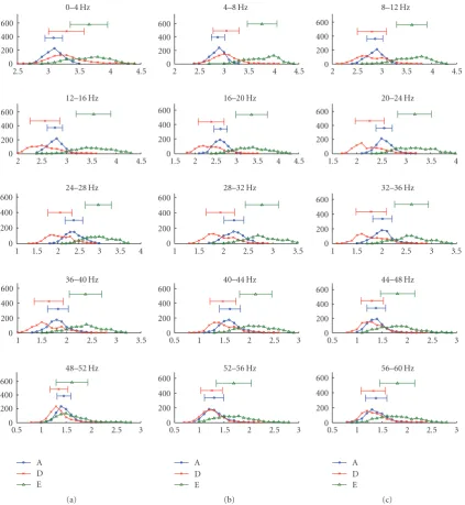
Figure 6shows the power distributions of the 15 subbands

(13)

0 200 400 600

0.5 1 1.5 2 2.5 3 48–52 Hz

0 200 400 600

1 1.5 2 2.5 3 3.5 36–40 Hz

0 200 400 600

1 1.5 2 2.5 3 3.5 4 24–28 Hz

0 200 400 600

2 2.5 3 3.5 4 4.5 12–16 Hz

0 200 400 600

2.5 3 3.5 4 4.5 0–4 Hz

A D E

(a)

0 200 400 600

0.5 1 1.5 2 2.5 3 52–56 Hz

0 200 400 600

0.5 1 1.5 2 2.5 3 40–44 Hz

0 200 400 600

1 1.5 2 2.5 3 3.5 28–32 Hz

0 200 400 600

1.5 2 2.5 3 3.5 4 4.5 16–20 Hz

0 200 400 600

2 2.5 3 3.5 4 4.5 4–8 Hz

A D E

(b)

0 200 400 600

0.5 1 1.5 2 2.5 3 56–60 Hz

0 200 400 600

0.5 1 1.5 2 2.5 3 44–48 Hz

0 200 400 600

1 1.5 2 2.5 3 3.5 32–36 Hz

0 200 400 600

1.5 2 2.5 3 3.5 4 20–24 Hz

0 200 400 600

2 2.5 3 3.5 4 4.5 8–12 Hz

A D E

(c)

Figure6: Power distributions of the 15 subbands corresponding to Set A (normal), Set D (interictal), and Set E (ictal).

linearly separate the three classes individually. Therefore, utilizing all of the subbands can lead to better performance.

Real-time operation is also an issue for an online seizure warning or seizure control system. The operations, includ-ing FFT analysis, approximate entropy analysis, and the LLS/LDA classification method, could be easily implemented on current processing platforms designed for various online applications. The results described here and in the literature

(Table 8) were obtained using a database selected and cut

out from continuous, multichannel EEG recordings after a visual inspection for artifacts such as muscle activity or eye movement. Further study to evaluate the performance of the seizure detection methods using continuous EEG recordings encompassing various behaviors and physiological states is required for development of clinical applications. In

addition, these methods may require modification if they are applied to other types of seizures, such as absence seizures that have rhythmic oscillations on fundamental and harmonic frequency bands of the scalp EEG [48,49].

Acknowledgment

This work was supported by the National Science Council of Taiwan under Grants nos. NSC 97-2627-B-006-005 and 98-2627-B-006-001.

References

(14)

[2] K. Lehnertz, F. Mormann, T. Kreuz, et al., “Seizure prediction by nonlinear EEG analysis,”IEEE Engineering in Medicine and Biology Magazine, vol. 22, no. 1, pp. 57–63, 2003.

[3] A. Subasi, “Epileptic seizure detection using dynamic wavelet network,”Expert Systems with Applications, vol. 29, no. 2, pp. 343–355, 2005.

[4] L. D. Iasemidis, “Epileptic seizure prediction and control,”

IEEE Transactions on Biomedical Engineering, vol. 50, no. 5, pp. 549–558, 2003.

[5] W. C. Stacey and B. Litt, “Technology insight: neuroengi-neering and epilepsy—designing devices for seizure control,”

Nature Clinical Practice Neurology, vol. 4, no. 4, pp. 190–201, 2008.

[6] L. D. Iasemidis, H. P. Zaveri, J. C. Sackellares, W. J. Williams, and T. W. Hood, “Nonlinear dynamics of electrocortico-graphic data,” Journal of Clinical Neurophysiology, vol. 5, p. 339, 1988.

[7] L. D. Iasemidis, J. C. Sackellares, H. P. Zaveri, and W. J. Williams, “Phase space topography and the lyapunov exponent of electrocorticograms in partial seizures,” Brain Topography, vol. 2, no. 3, pp. 187–201, 1990.

[8] N. Kannathal, M. L. Choo, U. R. Acharya, and P. K. Sadasivan, “Entropies for detection of epilepsy in EEG,” Computer Methods and Programs in Biomedicine, vol. 80, no. 3, pp. 187– 194, 2005.

[9] X. Li, G. Ouyang, and D. A. Richards, “Predictability anal-ysis of absence seizures with permutation entropy,”Epilepsy Research, vol. 77, no. 1, pp. 70–74, 2007.

[10] O. A. Rosso, S. Blanco, J. Yordanova, et al., “Wavelet entropy: a new tool for analysis of short duration brain electrical signals,”

Journal of Neuroscience Methods, vol. 105, no. 1, pp. 65–75, 2001.

[11] O. A. Rosso, “Entropy changes in brain function,” Interna-tional Journal of Psychophysiology, vol. 64, no. 1, pp. 75–80, 2007.

[12] V. Srinivasan, C. Eswaran, and N. Sriraam, “Approximate entropy-based epileptic EEG detection using artificial neural networks,” IEEE Transactions on Information Technology in Biomedicine, vol. 11, no. 3, pp. 288–295, 2007.

[13] P. Van Hese, J.-P. Martens, P. Boon, S. Dedeurwaerdere, I. Lemahieu, and R. Van de Walle, “Detection of spike and wave discharges in the cortical EEG of genetic absence epilepsy rats from Strasbourg,”Physics in Medicine and Biology, vol. 48, no. 12, pp. 1685–1700, 2003.

[14] V. Srinivasan, C. Eswaran, and A. N. Sriraam, “Artificial neural network based epileptic detection using time-domain and frequency-domain features,”Journal of Medical Systems, vol. 29, no. 6, pp. 647–660, 2005.

[15] R. Schuyler, A. White, K. Staley, and K. J. Cios, “Epileptic seizure detection,”IEEE Engineering in Medicine and Biology Magazine, vol. 26, no. 2, pp. 74–81, 2007.

[16] D. Bosnyakova, A. Gabova, A. Zharikova, V. Gnezditski, G. Kuznetsova, and G. van Luijtelaar, “Some peculiarities of time-frequency dynamics of spike-wave discharges in humans and rats,”Clinical Neurophysiology, vol. 118, no. 8, pp. 1736–1743, 2007.

[17] S. Ghosh-Dastidar, H. Adeli, and N. Dadmehr, “Mixed-band wavelet-chaos-neural network methodology for epilepsy and epileptic seizure detection,”IEEE Transactions on Biomedical Engineering, vol. 54, no. 9, pp. 1545–1551, 2007.

[18] S. Ghosh-Dastidar, H. Adeli, and N. Dadmehr, “Principal component analysis-enhanced cosine radial basis function

neural network for robust epilepsy and seizure detection,”

IEEE Transactions on Biomedical Engineering, vol. 55, no. 2, pp. 512–518, 2008.

[19] A. Alkan, E. Koklukaya, and A. Subasi, “Automatic seizure detection in EEG using logistic regression and artificial neural network,”Journal of Neuroscience Methods, vol. 148, no. 2, pp. 167–176, 2005.

[20] N. Acır, ˙I. ¨Oztura, M. Kuntalp, B. Baklan, and C. G¨uzelis¸, “Automatic detection of epileptiform events in EEG by a three-stage procedure based on artificial neural networks,” IEEE Transactions on Biomedical Engineering, vol. 52, no. 1, pp. 30– 40, 2005.

[21] R. G. Andrzejak, K. Lehnertz, F. Mormann, C. Rieke, P. David, and C. E. Elger, “Indications of nonlinear deterministic and finite-dimensional structures in time series of brain electrical activity: dependence on recording region and brain state,”

Physical Review E, vol. 64, Article ID 061907, 8 pages, 2001. [22] R. G. Andrzejak, “EEG time series download page,” http://

www.meb.uni-bonn.de/epileptologie/cms/upload/workgroup

/lehnertz/eegdata.html.

[23] V. P. Nigam and D. Graupe, “A neural-network-based detec-tion of epilepsy,”Neurological Research, vol. 26, no. 1, pp. 55– 60, 2004.

[24] K. Polat and S. G¨unes, “Classification of epileptiform EEG using a hybrid system based on decision tree classifier and fast Fourier transform,”Applied Mathematics and Computation, vol. 187, no. 2, pp. 1017–1026, 2007.

[25] A. Subasi, “EEG signal classification using wavelet feature extraction and a mixture of expert model,”Expert Systems with Applications, vol. 32, no. 4, pp. 1084–1093, 2007.

[26] A. T. Tzallas, M. G. Tsipouras, and D. I. Fotiadis, “Auto-matic seizure detection based on time-frequency analysis and artificial neural networks,” Computational Intelligence and Neuroscience, vol. 2007, Article ID 80510, 13 pages, 2007. [27] H. Ocak, “Optimal classification of epileptic seizures in

EEG using wavelet analysis and genetic algorithm,” Signal Processing, vol. 88, no. 7, pp. 1858–1867, 2008.

[28] N. F. Güler, E. D. Übeyli, and I. Güler, “Recurrent neural networks employing Lyapunov exponents for EEG signals classification,”Expert Systems with Applications, vol. 29, no. 3, pp. 506–514, 2005.

[29] N. Sadati, H. R. Mohseni, and A. Maghsoudi, “Epileptic seizure detection using neural fuzzy networks,” inProceedings of IEEE International Conference on Fuzzy Systems, pp. 596– 600, Vancouver, Canada, July 2006.

[30] S. R. Mousavi, M. Niknazar, and B. V. Vahdat, “Epileptic seizure detection using AR model on EEG signals,” in Proceed-ings of Cairo International Biomedical Engineering Conference (CIBEC ’08), pp. 1–4, Cairo, Egypt, December 2008.

[31] E. D. Übeyli and I. Güler, “Features extracted by eigenvector methods for detecting variability of EEG signals,” Pattern Recognition Letters, vol. 28, no. 5, pp. 592–603, 2007. [32] I. Güler and E. D. Übeyli, “Adaptive neuro-fuzzy inference

system for classification of EEG signals using wavelet coeﬃ -cients,”Journal of Neuroscience Methods, vol. 148, no. 2, pp. 113–121, 2005.

[33] I. G¨uler and E. D. ¨Ubeyli, “Multiclass support vector machines for EEG-signals classification,”IEEE Transactions on Informa-tion Technology in Biomedicine, vol. 11, no. 2, pp. 117–126, 2007.

(15)

Transactions on Information Technology in Biomedicine, vol. 13, no. 5, pp. 703–710, 2009.

[35] S. M. Pincus, “Approximate entropy as a measure of system complexity,”Proceedings of the National Academy of Sciences of the United States of America, vol. 88, no. 6, pp. 2297–2301, 1991.

[36] J. S. Richman and J. R. Moorman, “Physiological time-series analysis using approximate and sample entropy,” American Journal of Physiology, vol. 278, no. 6, pp. H2039–H2049, 2000. [37] C.-T. Lin, R.-C. Wu, T.-P. Jung, S.-F. Liang, and T.-Y. Huang, “Estimating driving performance based on EEG spectrum analysis,”EURASIP Journal on Applied Signal Processing, vol. 2005, no. 19, pp. 3165–3174, 2005.

[38] N. V. Thakor and S. Tong, “Advances in quantitative electroen-cephalogram analysis methods,”Annual Review of Biomedical Engineering, vol. 6, pp. 453–495, 2004.

[39] S. M. Kay,Modern Spectral Estimation: Theory and Application, Prentice Hall, Hall Englewood Cliﬀs, NJ, USA, 1988. [40] M. Mitchell,An Introduction to Genetic Algorithms, MIT Press,

Cambriduge, Mass, USA, 1988.

[41] G. Golub, “Numerical methods for solving linear least squares problems,”Numerische Mathematik, vol. 7, no. 3, pp. 206–216, 1965.

[42] L. B. Friedman, “Regularized discriminant analysis,”Journal of the American Statistical Association, vol. 84, no. 405, pp. 165– 175, 1989.

[43] D. E. Rumelhart, G. E. Hinton, and R. J. Williams, “Learning representations by back-propagating errors,”Nature, vol. 323, no. 6088, pp. 533–536, 1986.

[44] C. Cortes and V. Vapnik, “Support-vector networks,”Machine Learning, vol. 20, no. 3, pp. 273–297, 1995.

[45] B.-C. Kuo and D. A. Landgrebe, “Nonparametric weighted feature extraction for classification,” IEEE Transactions on Geoscience and Remote Sensing, vol. 42, no. 5, pp. 1096–1105, 2004.

[46] C.-T. Lin, K.-L. Lin, L.-W. Ko, S.-F. Liang, B.-C. Kuo, and I.-F. Chung, “Nonparametric single-trial EEG feature extraction and classification of driver’s cognitive responses,”EURASIP Journal on Applied Signal Processing, vol. 2008, Article ID 849040, 10 pages, 2008.

[47] C.-T. Lin, C.-M. Yeh, S.-F. Liang, J.-F. Chung, and N. Kumar, “Support-vector-based fuzzy neural network for pattern clas-sification,”IEEE Transactions on Fuzzy Systems, vol. 14, no. 1, pp. 31–41, 2006.

[48] X. Li, G. Ouyang, and D. A. Richards, “Predictability anal-ysis of absence seizures with permutation entropy,”Epilepsy Research, vol. 77, no. 1, pp. 70–74, 2007.

[49] F.-Z. Shaw, “Is spontaneous high-voltage rhythmic spike discharge in Long Evans rats an absence-like seizure activity?”